Posterior Average Effects

Abstract

Economists are often interested in estimating averages with respect to distributions of unobservables, such as moments of individual fixed-effects, or average partial effects in discrete choice models. For such quantities, we propose and study posterior average effects (PAE), where the average is computed conditional on the sample, in the spirit of empirical Bayes and shrinkage methods. While the usefulness of shrinkage for prediction is well-understood, a justification of posterior conditioning to estimate population averages is currently lacking. We show that PAE have minimum worst-case specification error under various forms of misspecification of the parametric distribution of unobservables. In addition, we introduce a measure of informativeness of the posterior conditioning, which quantifies the worst-case specification error of PAE relative to parametric model-based estimators. As illustrations, we report PAE estimates of distributions of neighborhood effects in the U.S., and of permanent and transitory components in a model of income dynamics.

Keywords:

• Empirical Bayes
• Latent variables
• Model misspecification
• Posterior conditioning
• Robustness
• Sensitivity analysis

1 Introduction

In many settings, applied researchers wish to estimate population averages with respect to a distribution of unobservables. This includes moments of individual fixed-effects in panel data, and average partial effects in discrete choice models, which are expectations with respect to some distribution of shocks or heterogeneity. The standard approach in applied work is to assume a parametric form for the distribution of unobservables, and to compute the average effect under that assumption. For example, in binary choice, researchers often assume normality of the error term, and compute average partial effects under normality. This “model-based” estimation of average effects is justified under the assumption that the parametric model is correctly specified.

In this article, we consider a different approach, where the average effect is computed conditional on the observation sample. We refer to such estimators as “posterior average effects” (PAE). Posterior averaging is appealing for prediction purposes, and it plays a central role in Bayesian and empirical Bayes (EB) approaches (e.g., Berger 1980; Morris 1983). Here, we focus instead on the estimation of population expectations. Our goal is twofold: to propose a novel class of estimators, and to provide a frequentist framework to understand when and why posterior conditioning may be useful in estimation. Our main result will show that PAE have robustness properties when the parametric model is misspecified.

PAE are closely related to EB estimators, which are increasingly popular in applied economics. Consider a fixed-effects model of teacher quality, which is our main example. When the number of observations per teacher is small, the dispersion of teacher fixed-effects is likely to overstate that of true teacher quality, since teacher effects are estimated with noise. An alternative approach is to postulate a prior distribution for teacher quality—typically, a normal—and report posterior estimates, holding fixed the values of the mean and variance parameters. The hope is that such EB estimates, which are shrunk toward the prior, are less affected by noise than the teacher fixed-effects (e.g., Kane and Staiger 2008; Chetty et al. 2014; Angrist et al. 2017). However, while EB estimates are well-justified predictors of the quality of individual teachers, it is not obvious how to aggregate them across teachers when the goal is to estimate a population average such as a moment or a distribution function.

As an example, suppose we wish to estimate the distribution function of teacher quality evaluated at a point. Since this quantity is an average of indicator functions, the PAE is simply an average of posterior means—that is, of EB estimates—of the indicator functions. This estimator is available in closed form. However, the PAE differs from the empirical distribution of the EB estimates of teacher effects. In particular, while the variance of EB estimates is too small relative to that of latent teacher quality, the PAE has the correct variance. Related applications of PAE include settings involving neighborhood/place effects (Chetty and Hendren 2018; Finkelstein et al. 2017) or hospital quality (Hull 2018).

Importantly, although posterior averages have desirable properties for predicting individual parameters, their usefulness for estimating population average quantities is not evident. For example, suppose that teacher quality is normally distributed. In this case, a model-based normal estimator of the distribution of teacher quality is consistent. Moreover, it is asymptotically efficient when means and variances are estimated by maximum likelihood. Hence, in the correctly specified case, there is no reason to deviate from the standard model-based approach and compute posterior estimators. The main insight of this article is that, under misspecification—for example, when teacher quality is not normally distributed—conditioning on the data using PAE can be beneficial.

To study estimators under misspecification, we focus on specification error, which is the population discrepancy between the probability limit of an estimator and the true parameter value. In our main results, we show that PAE have minimum worst-case specification error, where the worst case is computed in a nonparametric neighborhood of the reference parametric distribution (e.g., a normal). Specifically, we show that, when neighborhoods are defined in terms of the Pearson chi-squared divergence, PAE have minimum worst-case specification error within a large class of estimators, for any neighborhood size smaller than a threshold value that we characterize. In addition, when broadening the class of neighborhoods to $\varphi$-divergences, we show that, while PAE do not have minimum worst-case specification error in general in fixed-size neighborhoods, they achieve minimum worst-case specification error under local misspecification, that is, when the size of the neighborhood tends to zero.

In our examples and illustrations, we find that the information contained in the posterior conditioning is setting-specific. This is intuitive, since although PAE have minimum worst-case specification error under our conditions, the specification error is not zero in general and it varies between applications. PAE tend to behave better when the realizations of outcome variables (such as test scores) are more informative about the values of the unobservables (such as the quality of a teacher). Consistently with this intuition, our local result suggests quantifying the “informativeness” of the posterior conditioning using an easily computable R² coefficient.

While our theoretical results focus on population specification error, in practice PAE are also affected by sampling error, due to the fact that the sample size—for example, the number of teachers—is not infinite. A common approach to account for both sampling variability and specification error is to focus on mean squared error. In general, PAE do not have minimum mean squared error: indeed, in finite samples, model-based estimators can have smaller mean squared error than PAE. In Bonhomme and Weidner (2018), we show how to construct estimators that minimize mean squared error under local asymptotic misspecification. However, such estimators depend on the neighborhood size. In contrast, PAE do not require taking a stand on the degree of misspecification through the size of the neighborhood, and they are simple to implement and do not depend on tuning parameters. To complement the theory, we report the results of a Monte Carlo simulation, where we compare the performance of the PAE to those of a model-based estimator and a nonparametric deconvolution-based estimator. We find that, while the model-based estimator tends to perform best under correct specification, the performance of the PAE appears less sensitive to misspecification than those of the model-based and nonparametric estimators.

To illustrate the scope of PAE for applications, we then consider two empirical settings. In the first one, we study the estimation of neighborhood/place effects in the United States. Chetty and Hendren (2018) reported estimates of the variance of neighborhood effects, as well as EB estimates of those effects. Our goal is to estimate the distribution of effects across neighborhoods. We find that, when using a normal prior as in Chetty and Hendren (2018), our posterior estimator of the distribution function of neighborhood effects across commuting zones is not normal. However, we also show through simulations and computation of our posterior informativeness measure that the signal-to-noise ratio in the data is not high enough to be confident about the exact shape of the distribution. Hence, in this setting, PAE inform our knowledge of the distribution of neighborhood effects, and motivate future analyses using more flexible model specifications and individual-level data.

In the second empirical illustration, our goal is to estimate the distributions of latent components in a permanent-transitory model of income dynamics (e.g., Hall and Mishkin 1982; Blundell et al. 2008), where log-income is the sum of a random-walk component and a component that is independent over time. Researchers often estimate the covariance structure of the latent components in a first step. Then, in order to document distributions or to use the income process in a consumption-saving model, they often assume Gaussianity. However, there is increasing evidence that income components are not Gaussian (e.g., Geweke and Keane 2000; Hirano 2002; Bonhomme and Robin 2010; Guvenen et al. 2016). We estimate posterior distribution functions of permanent and transitory income components using recent waves from the Panel Study of Income Dynamics (PSID). Our PAE estimates suggest some departure from Gaussianity, especially for the transitory income component.

We analyze several extensions. First, we describe the form of PAE in several models, including binary choice and censored regression. Second, we discuss how to construct confidence intervals and specification tests based on PAE. Lastly, we revisit the question of optimality of EB estimates for predicting individual parameters. By extending our misspecification analysis from worst-case specification error of sample averages to worst-case mean squared prediction error, we show that EB estimators remain optimal, up to small-order terms, under local deviations from normality.

1.1 Related Literature and Outline

PAE are closely related to parametric EB estimators (Efron and Morris 1973; Morris 1983). For the recent econometric applications of shrinkage methods (James and Stein 1961; Efron 2012), see Hansen (2016), Fessler and Kasy (2018), and Abadie and Kasy (2018). Recent contributions to nonparametric EB methods are Koenker and Mizera (2014) and Ignatiadis and Wager (2019).

Our analysis is also related to deconvolution and other nonparametric approaches. However, in our framework we allow for forms of misspecification under which the quantity of interest is not consistently estimable, and we search for estimators that have the smallest specification error.

In panel data settings, Arellano and Bonhomme’s (2009) study the asymptotic properties of random-effects estimators of averages of functions of covariates and individual effects. They show that, when the distribution of individual effects is misspecified, whereas the other features of the model are correctly specified, PAE are consistent as n and T tend to infinity. By contrast, in our setup, only n tends to infinity, and misspecification may affect the entire joint distribution of unobservables.

Our analysis also connects to the literature on robustness to model misspecification (e.g., Huber and Ronchetti 2009; Kitamura et al. 2013; Andrews et al. 2017, 2020; Armstrong and Kolesár 2018; Bonhomme and Weidner 2018; Christensen and Connault 2019). Here, our aim is to propose and justify a class of simple, practical estimators.

The plan of the article is as follows. In Section 2, we motivate the analysis by considering a fixed-effects model of teacher quality. In Section 3, we present our framework and derive our main theoretical results. In Section 4, we illustrate the use of PAE in two empirical settings. In Section 5, we describe several extensions. Finally, we conclude in Section 6. Replication codes are available as online material.

2 Motivating Example: A Fixed-Effects Model

To motivate the analysis, we start by considering the following model:(1) $$Y_{ij}={\alpha }_i+{\epsilon }_{ij},\mathrm{\hspace{1em}}\mathrm{\hspace{1em}}\hspace{1em}i=1,\dots ,n,\mathrm{\hspace{1em}}\mathrm{\hspace{1em}}j=1,\dots ,J.$$(1)

To fix ideas, we will think of Y_ij as an average test score of teacher i in classroom j, α_i as the quality of teacher i, and ${\epsilon }_{ij}$ as a classroom-specific shock. There are n teachers and J observations per teacher. For simplicity, we abstract away from covariates (such as students’ past test scores), but those will be present in the framework we will introduce in the next section. Although here we focus on teacher effects, this model is of interest in other settings, such as the study of neighborhood effects, school effectiveness, or hospital quality, for example.

Suppose we wish to estimate a feature of the distribution of teacher quality α. As an example, here we consider the distribution function of α at a particular point a,$$F_{\alpha }(a)=\mathbb{E}\left[\mathbf{1}\{\alpha \le a\}\right],$$which is the percentage of teachers whose quality is below a. A first estimator is the empirical distribution of the fixed-effects estimates ${\widehat{\alpha }}_i={\overline{Y}}_i=\frac{1}{J}{\sum }_{j=1}^J{Y}_{ij}$, for all teachers $i=1,\dots ,n$; that is,(2) $${\widehat{F}}_{\alpha }^{\text{FE}}(a)=\frac{1}{n}\sum _{i=1}^n\mathbf{1}\{{\overline{Y}}_i\le a\},$$(2) where FE stands for “fixed-effects.” An obvious issue with this estimator is that ${\overline{Y}}_i={\alpha }_i+{\overline{\epsilon }}_i$ is a noisy estimate of α_i, where ${\overline{\epsilon }}_i=\frac{1}{J}{\sum }_{j=1}^J{\epsilon }_{ij}$. Indeed, due to the presence of noise, for fixed J and n tends to infinity the distribution ${\widehat{F}}_{\alpha }^{\text{FE}}$ tends to be too dispersed relative to $F_{\alpha }$ (although one can show that ${\widehat{F}}_{\alpha }^{\text{FE}}(a)$ is consistent for $F_{\alpha }(a)$ as J tends to infinity jointly with n under mild conditions; see Jochmans and Weidner 2018).

A different strategy is to model the joint distribution of $\alpha ,{\epsilon }_1,\dots ,{\epsilon }_J$. A simple specification is a multivariate normal distribution with means ${\mu }_{\alpha }$ and ${\mu }_{\epsilon }=0$, and variances $s_{\alpha }^2$ and $s_{\epsilon }^2$. This specification can easily be made more flexible by allowing for different $s_{{\epsilon }_j}^2$’s across j, for correlation between the different ${\epsilon }_j$’s, or for means and variances being functions of covariates, for example. Under the assumption that all components are uncorrelated, ${\mu }_{\alpha },s_{\alpha }^2$, and $s_{\epsilon }^2$ can be consistently estimated for fixed J as n tends to infinity, using quasi-maximum likelihood or minimum distance based on mean and covariance restrictions.

Given estimates ${\widehat{\mu }}_{\alpha },{\widehat{s}}_{\alpha }^2,{\widehat{s}}_{\epsilon }^2$, we can compute EB estimates (Morris 1983) of the α_i as(3) $$\mathbb{E}[\alpha |Y=Y_i]={\widehat{\mu }}_{\alpha }+\widehat{\rho }({\overline{Y}}_i-{\widehat{\mu }}_{\alpha }),\hspace{1em}i=1,\dots ,n,$$(3) where the expectation is taken with respect to the posterior distribution of α given Y = Y_i for ${\widehat{\mu }}_{\alpha },{\widehat{s}}_{\alpha }^2,{\widehat{s}}_{\epsilon }^2$ fixed, and $\widehat{\rho }=\frac{{\widehat{s}}_{\alpha }^2}{{\widehat{s}}_{\alpha }^2+{\widehat{s}}_{\epsilon }^2/J}$ is a shrinkage factor. Here, Y_i are vectors containing all Y_ij, $j=1,\dots ,J$. The EB estimates in (3) are well-justified as predictors of the α_i, since (when treating ${\widehat{\mu }}_{\alpha },{\widehat{s}}_{\alpha }^2,{\widehat{s}}_{\epsilon }^2$ as fixed) ${\widehat{\mu }}_{\alpha }+\widehat{\rho }({\overline{Y}}_i-{\widehat{\mu }}_{\alpha })$ is the minimum mean squared error predictor of α_i under normality.

Given their rationale for prediction purposes, it is appealing to try and aggregate the EB estimates in order to estimate our target quantity $F_{\alpha }(a)$. A possible estimator is(4) $${\widehat{F}}_{\alpha }^{\text{PM}}(a)=\frac{1}{n}\sum _{i=1}^n\mathit{1}\left\{{\widehat{\mu }}_{\alpha }+\widehat{\rho }({\overline{Y}}_i-{\widehat{\mu }}_{\alpha })\le a\right\},$$(4) where PM stands for “posterior means.” For fixed J as n tends to infinity, the EB estimates tend to be less dispersed than the true α_i, and ${\widehat{F}}_{\alpha }^{\text{PM}}(a)$ is inconsistent in general. Indeed, while in large samples the variance of the fixed-effects estimates is ${\rho }^{-1}{s}_{\alpha }^2>s_{\alpha }^2$, the variance of the EB estimates is $\rho s_{\alpha }^2<s_{\alpha }^2$, where $\rho =\frac{s_{\alpha }^2}{s_{\alpha }^2+s_{\epsilon }^2/J}$.

Instead of computing the distribution of EB estimates as in Equation (4)(4) $${\widehat{F}}_{\alpha }^{\text{PM}}(a)=\frac{1}{n}\sum _{i=1}^n\mathit{1}\left\{{\widehat{\mu }}_{\alpha }+\widehat{\rho }({\overline{Y}}_i-{\widehat{\mu }}_{\alpha })\le a\right\},$$(4) , a related idea is to compute the posterior distribution estimator$${\widehat{F}}_{\alpha }^{\mathrm{P}}(a)=\frac{1}{n}\sum _{i=1}^n\mathbb{E}\left[\mathit{1}\{\alpha \le a\}|Y=Y_i\right],$$

where P stands for “posterior.” Using the normality assumption, we obtain(5) $${\widehat{F}}_{\alpha }^{\mathrm{P}}(a)=\frac{1}{n}\sum _{i=1}^n\Phi \left(\frac{a-{\widehat{\mu }}_{\alpha }-\widehat{\rho }({\overline{Y}}_i-{\widehat{\mu }}_{\alpha })}{{\widehat{s}}_{\alpha }\sqrt{1-\widehat{\rho }}}\right),$$(5) where $\Phi$ denotes the distribution function of the standard normal. ${\widehat{F}}_{\alpha }^{\mathrm{P}}(a)$ is an example of a PAE. One can check that it is consistent for fixed J as n tends to infinity, when the distribution of $\alpha ,{\epsilon }_1,\dots ,{\epsilon }_J$ is normal. Under nonnormality, ${\widehat{F}}_{\alpha }^{\mathrm{P}}(a)$ is generally inconsistent for fixed J as n tends to infinity. Moreover, the mean and variance of ${\widehat{F}}_{\alpha }^{\mathrm{P}}$ are $(1-\widehat{\rho }){\widehat{\mu }}_{\alpha }+\widehat{\rho }\frac{1}{n}{\sum }_{i=1}^n{\overline{Y}}_i$ and $(1-\widehat{\rho }){\widehat{s}}_{\alpha }^2+{\widehat{\rho }}^2\left[\frac{1}{n}{\sum }_{i=1}^n{\overline{Y}}_i^2-{(\frac{1}{n}{\sum }_{i=1}^n{\overline{Y}}_i)}^2\right]$, respectively, which are consistent for ${\mu }_{\alpha }$ and $s_{\alpha }^2$ for fixed J as n tends to infinity.

The last estimator we consider here is directly based on the normal specification for α,(6) $${\widehat{F}}_{\alpha }^{\mathrm{M}}(a)=\Phi \left(\frac{a-{\widehat{\mu }}_{\alpha }}{{\widehat{s}}_{\alpha }}\right),$$(6) where M stands for “model.” This estimator enjoys attractive properties when the distribution of $\alpha ,{\epsilon }_1,\dots ,{\epsilon }_J$ is indeed normal. In this case, ${\widehat{F}}_{\alpha }^{\mathrm{M}}(a)$ is consistent for fixed J as n tends to infinity, and it is efficient when ${\widehat{\mu }}_{\alpha }$ and ${\widehat{s}}_{\alpha }^2$ are maximum likelihood estimates. Moreover, the mean and variance of ${\widehat{F}}_{\alpha }^{\mathrm{M}}$ are ${\widehat{\mu }}_{\alpha }$ and ${\widehat{s}}_{\alpha }^2$, which are consistent irrespective of normality. However, when $\alpha ,{\epsilon }_1,\dots ,{\epsilon }_J$ is not normally distributed, ${\widehat{F}}_{\alpha }^{\mathrm{M}}(a)$ is generally inconsistent for fixed J as n tends to infinity. Moreover, ${\widehat{F}}_{\alpha }^{\mathrm{M}}(a)$ only depends on the data through the mean ${\widehat{\mu }}_{\alpha }$ and the variance ${\widehat{s}}_{\alpha }^2$. In particular, ${\widehat{F}}_{\alpha }^{\mathrm{M}}$ is always normal, even when the data show clear evidence of nonnormality.

Which one of these estimators should one use? The answer is not obvious, since they are all inconsistent as n tends to infinity for fixed J in general. In a framework that allows for misspecification of the normal distribution of $\alpha ,{\epsilon }_1,\dots ,{\epsilon }_J$, we will show that the PAE ${\widehat{F}}_{\alpha }^{\mathrm{P}}(a)$ has minimum worst-case specification error in certain neighborhoods around the normal reference distribution. To our knowledge, unlike the other three estimators above, posterior estimators of distributions are novel to practitioners. They are easy to implement, and do not depend on additional tuning parameters. Our characterization provides a rationale for reporting them in applications, alongside other parametric and semiparametric estimators.

Note that one may wish to relax normality by making the specification of α, and possibly ${\epsilon }_j$, more flexible. Deconvolution and nonparametric maximum likelihood estimators are often used for this purpose (e.g., Delaigle et al. 2008; Bonhomme and Robin 2010; Koenker and Mizera 2014). While these estimators may be consistent even when α is not normal, consistency relies on additional restrictions on the model. For example, the assumptions in Kotlarski (1967) require that α, ${\epsilon }_1$, …, ${\epsilon }_J$ be mutually independent. By contrast, we do not impose any such additional conditions in our framework. In Section 3, we will show that asymptotically linear estimators have larger specification error than PAE under the form of misspecification that we consider.

To illustrate that an independence assumption among α, ${\epsilon }_1$, …, ${\epsilon }_J$ can be restrictive, consider a situation where the researcher is concerned that the variance of ${\epsilon }_j$ depends on α. For instance, the variance of classroom-level shocks may depend on teacher quality. The presence of such conditional heteroscedasticity would invalidate conventional nonparametric deconvolution estimators. By contrast, we will show that ${\widehat{F}}_{\alpha }^{\mathrm{P}}(a)$ has minimum specification error in neighborhoods of distributions that allow for conditional heteroscedasticity. In Section 4 and the appendix, we will compare the finite-sample behavior of the parametric model-based estimator, the PAE, and a nonparametric deconvolution estimator, in data simulated from various specifications of model (1).

In model (1), the researcher may be interested in estimating other quantities. As an example, consider the coefficient in the population regression of teacher quality α on a vector of covariates W; that is,(7) $$\overline{\delta }={\left(\mathbb{E}[WW\prime ]\right)}^{-1}\mathbb{E}\left[W\alpha \right].$$(7)

In applications, it is common to regress fixed-effects estimates on covariates to help interpret them (as in Dobbie and Fryer 2013; among many others), and to compute(8) $${\widehat{\delta }}^{\text{FE}}={\left(\sum _{i=1}^n{W}_i{W}_i^{\prime }\right)}^{-1}\sum _{i=1}^n{W}_i{\overline{Y}}_i.$$(8)

Alternatively, one may regress the EB estimates of α_i, as given by (3), on covariates (as in Angrist et al. 2017, and Hull 2018, for example), and compute(9) $${\widehat{\delta }}^{\mathrm{P}}={\left(\sum _{i=1}^n{W}_i{W}_i^{\prime }\right)}^{-1}\sum _{i=1}^n{W}_i\left({\widehat{\mu }}_{\alpha }+\widehat{\rho }({\overline{Y}}_i-{\widehat{\mu }}_{\alpha })\right),$$(9) which is a PAE based on a normal reference specification for α. We will see that, in our framework, the rationale for reporting ${\widehat{\delta }}^{\mathrm{P}}$ or ${\widehat{\delta }}^{\text{FE}}$ depends on the form of misspecification that the researcher is concerned about.

The framework we describe next applies to the estimation of different quantities in a variety of settings. In Section 4 we apply PAE to model (1) and estimate the distribution of neighborhood/place effects in the U.S. (Chetty and Hendren 2018). In addition, we show that the permanent-transitory model of income dynamics (e.g., Hall and Mishkin 1982) has a structure similar to model (1), and we report PAE estimates in this context. Last, in other models—such as static or dynamic discrete choice models and models with censored outcomes—our results motivate the use of PAE as complements to other estimators that researchers commonly report, and we provide examples in Section 5 and analyze them in the appendix.

3 Framework and Main Results

In this section we describe our framework to study PAE, and present our main results.

3.1 Model-Based Estimators and PAE

We consider the following class of models:(10) $$Y_i=g_{\beta }(U_i,X_i),$$(10) where outcomes Y_i and covariates X_i are observed by the researcher, and U_i are unobserved. The function $g_{\beta }$ is known up to the finite-dimensional parameter β. Our aim is to estimate an average effect of the form(11) $$\overline{\delta }={\mathbb{E}}_{f_0}\left[{\delta }_{\beta }(U,X)\right],$$(11) where ${\delta }_{\beta }$ is scalar, and known given β. Here, f₀ denotes the true density of $U|X$. The expectation is taken with respect to the product $f_0{f}_X$, where f_X is the marginal density of X. For conciseness we leave the dependence on f_X implicit. While we focus on a scalar ${\delta }_{\beta }$, our results continue to hold in the vector-valued case, as we show at the end of this section. In Appendix S5, we discuss how to estimate quantities that depend on f₀ nonlinearly.

While the researcher does not know the true f₀, she has a reference parametric density $f_{\sigma }$ for $U|X$, which depends on a finite-dimensional parameter σ. We will allow $f_{\sigma }$ to be misspecified, in the sense that f₀ may not belong to $\left\{f_{\sigma }\right\}$. However, we will always assume that $g_{\beta }$ is correctly specified. In other words, misspecification will only affect the distribution of U and its dependence on X, not the structural link between (U, X) and outcomes.

To estimate $\overline{\delta }$ in Equaiton (11), we assume that the researcher has an estimator $\widehat{\beta }$ that remains consistent for β under misspecification of $f_{\sigma }$. More precisely, we will only consider potential true densities f₀ such that $\widehat{\beta }$ tends in probability to the true value β under f₀. For example, in the fixed-effects model (1), consistent estimates of means and variances can be obtained in the absence of normality.

To map model (1) to the general notation of this section, note that in this case there are no covariates X, and the vector of unobservables U is$$U=\left(\frac{\alpha -{\mu }_{\alpha }}{s_{\alpha }},\frac{{\epsilon }_1}{s_{\epsilon }},\dots ,\frac{{\epsilon }_J}{s_{\epsilon }}\right)\prime .$$

The vector β is $\beta =({\mu }_{\alpha },s_{\alpha }^2,s_{\epsilon }^2)\prime$. The reference distribution for U is a standard multivariate normal, so the reference density $f_{\sigma }$ is known in this case — in other words, the parameter σ in $f_{\sigma }$ can be omitted. We assume that the researcher has computed an estimator $\widehat{\beta }$, for example by quasi-maximum likelihood or minimum distance, which remains consistent for β when U is not normally distributed.

In certain applications, the reference density depends on some parameters σ that cannot be consistently estimated absent parametric assumptions. In Appendix S6, we describe discrete choice and censored regression models that have this structure. In such settings, we assume that the researcher has an estimator $\widehat{\sigma }$ that tends in probability to some ${\sigma }_{*}$ under f₀. Unlike β, the parameter ${\sigma }_{*}$ is a model-specific “pseudo-true value” that is not assumed to have generated the data. However, in our leading example of model (1), as well as in the model’s generalizations that we study in our empirical illustrations in Section 4, the references to $\widehat{\sigma }$ and ${\sigma }_{*}$ can be omitted from all subsequent statements and derivations.

Given $\widehat{\beta },\widehat{\sigma }$, a sample $\{Y_i,X_i,i=1,\dots ,n\}$ from (Y, X), and the parametric density $f_{\sigma }$, a model-based estimator of $\overline{\delta }$ is(12) $${\widehat{\delta }}^{\mathrm{M}}=\frac{1}{n}\sum _{i=1}^n{\mathbb{E}}_{f_{\widehat{\sigma }}}\left[{\delta }_{\widehat{\beta }}(U,X)|X=X_i\right],$$(12) where, with some abuse of notation, the expectation with respect to $f_{\widehat{\sigma }}$ is computed only over U. When not available in closed form, this estimator can be computed by numerical integration or simulation under the parametric density $f_{\widehat{\sigma }}$. It is easy to see that, under standard conditions, ${\widehat{\delta }}^{\mathrm{M}}$ is consistent for $\overline{\delta }$ under correct specification; that is, when $f_{{\sigma }_{*}}$ is the true density of $U|X$.

To construct a posterior estimator, consider the posterior density $p_{\beta ,\sigma }$ of $U|Y,X$. This posterior density is computed using Bayes rule, based on the prior $f_{\sigma }$ on $U|X$ and the likelihood of $Y|U,X$ implied by $g_{\beta }$. Formally, let $\mathcal{U}(y,x,\beta )=\{u:y=g_{\beta }(u,x)\}$. We define, whenever the denominator is non-zero,(13) $$p_{\beta ,\sigma }(u|y,x)=\frac{f_{\sigma }(u|x)\mathbf{1}\{u\in \mathcal{U}(y,x,\beta )\}}{\int f_{\sigma }(v|x)\mathbf{1}\{v\in \mathcal{U}(y,x,\beta )\}dv}.$$(13)

We will compute $p_{\beta ,\sigma }$ analytically in our examples. In Appendix S5 we describe a simulation-based computational approach when an analytical expression is not available. We define the PAE as the posterior estimator(14) $${\widehat{\delta }}^{\mathrm{P}}=\frac{1}{n}\sum _{i=1}^n{\mathbb{E}}_{p_{\widehat{\beta },\widehat{\sigma }}}\left[{\delta }_{\widehat{\beta }}(U,X)|Y=Y_i,X=X_i\right],$$(14) where, again, the expectation is only taken over U. Under standard regularity conditions, it is easy to see that, like ${\widehat{\delta }}^{\mathrm{M}}$, the PAE ${\widehat{\delta }}^{\mathrm{P}}$ is consistent for $\overline{\delta }$ under correct specification.

From a Bayesian perspective, ${\widehat{\delta }}^{\mathrm{P}}$ is a natural estimator to consider when β and σ are known. Indeed, ${\widehat{\delta }}^{\mathrm{P}}$ is then the posterior mean of $\frac{1}{n}{\sum }_{i=1}^n{\delta }_{\beta }(U_i,X_i)$, where the prior on U_i is $f_{\sigma }$, independent across i. An alternative Bayesian interpretation is obtained by specifying a nonparametric prior on f₀, and computing the posterior mean of $\overline{\delta }$ under this prior, as we discuss in Appendix S5 in the case where U has finite support. However, a frequentist justification for ${\widehat{\delta }}^{\mathrm{P}}$ appears to be lacking in the literature. Indeed, under correct specification of $f_{\sigma }$, both estimators ${\widehat{\delta }}^{\mathrm{P}}$ and ${\widehat{\delta }}^{\mathrm{M}}$ are consistent, and, as we pointed out in the previous section, ${\widehat{\delta }}^{\mathrm{P}}$ may have a higher variance than ${\widehat{\delta }}^{\mathrm{M}}$. The key difference between model-based and posterior estimators is that ${\widehat{\delta }}^{\mathrm{P}}$ is conditional on the observation sample. An intuitive rationale for the conditioning is the recognition that realizations Y_i may be informative about the values of the unknown U_i’s. We next formalize this intuition in a framework that accounts for specification error.

3.2 Neighborhoods, Estimators, and Worst-Case Specification Error

Let $P(\beta ,f_0)$ denote the true density of (Y, U, X), where as before we omit the reference to the marginal density of X for conciseness. We assume that, under $P(\beta ,f_0),\widehat{\beta }$ is consistent for the true β, and $\widehat{\sigma }$ is consistent for a model-specific “pseudo-true” value ${\sigma }_{*}$, where ${\mathbb{E}}_{P(\beta ,f_0)}[{\psi }_{\beta ,{\sigma }_{*}}(Y,X)]=0$ for some moment function ψ. For example, $\widehat{\beta }$ and $\widehat{\sigma }$ may be the method-of-moments estimators that solve ${\sum }_{i=1}^n{\psi }_{\widehat{\beta },\widehat{\sigma }}(Y_i,X_i)=0$. In models with no σ parameters, such as model (1) and its generalizations, we only assume that $\widehat{\beta }$ is consistent for β, and that ${\mathbb{E}}_{P(\beta ,f_0)}[{\psi }_{\beta }(Y,X)]=0$ for some ψ. Throughout, we take the estimators $\widehat{\beta }$ (and possibly $\widehat{\sigma }$), and the moment function ψ, as given. In particular, we do not address the question of optimal estimation of β under misspecification.

Given a distance measure d and a scalar $ϵ\ge 0$, we define the following neighborhood of the reference density $f_{\sigma }$:$${\Gamma }_{ϵ}=\left\{f_0:d(f_0,f_{{\sigma }_{*}})\le ϵ,{\mathbb{E}}_{P(\beta ,f_0)}[{\psi }_{\beta ,{\sigma }_{*}}(Y,X)]=0\right\}.$$

This neighborhood consists of densities of $U|X$ that are at most ϵ away from $f_{{\sigma }_{*}}$, and under which $\widehat{\beta }$ and $\widehat{\sigma }$ converge asymptotically to β and ${\sigma }_{*}$, respectively. The case ϵ = 0 corresponds to correct specification of the reference density, whereas $ϵ>0$ corresponds to misspecification.

For ease of notation we omit the dependence of ${\Gamma }_{ϵ}$ on β, ${\sigma }_{*}$, and ψ, all of which we consider fixed and given in this section. Indeed, we assume that the researcher has chosen an estimator $\widehat{\beta }$, and, depending on the setting, an estimator $\widehat{\sigma }$—our theory is silent about where these choices come from—and that she has already observed their realized values in a large sample. The moment function ψ is determined by this choice of estimators. Moreover, in large samples, the population values β and ${\sigma }_{*}$ are arbitrarily close to the observed values $\widehat{\beta }$ and $\widehat{\sigma }$. In our setup, we only consider densities of unobservables f₀ that are consistent with those values, in the sense that the moment restriction ${\mathbb{E}}_{P(\beta ,f_0)}[{\psi }_{\beta ,{\sigma }_{*}}(Y,X)]=0$ holds. This large-sample logic is consistent with our focus on specification error; see (16) below.

Note that the same logic might suggest imposing that other features of the joint population distribution of the data (Y, X), such as means, covariances, higher-order moments, or even the entire distribution, be kept constant for all $f_0\in {\Gamma }_{ϵ}$. Restricting neighborhoods in this way does not affect the results in this section, because those are valid for all possible ψ, and one could thus impose additional moment restrictions on f₀.

Let us denote the supports of X and U as $\mathcal{X}$ and $\mathcal{U}$, respectively. We assume that d is a $\varphi$-divergence of the form$$d(f_0,f_{\sigma })={\int }_{\mathcal{X}}{\int }_{\mathcal{U}}\varphi \left(\frac{f_0(u|x)}{f_{\sigma }(u|x)}\right)f_{\sigma }(u|x)f_X(x)dudx,$$where $\varphi$ is a convex function that satisfies $\varphi (1)=0$ and $\varphi ″(1)>0$. This family contains as special cases the ${\chi }^2$ divergence (averaged over X), the Kullback–Leibler divergence, the Hellinger distance, and more generally the members of the Cressie-Read family of divergences (Cressie and Read 1984). It is commonly used to measure misspecification, see Andrews et al. (2020) and Christensen and Connault (2019) for recent examples.

We focus on asymptotically linear estimators of $\overline{\delta }$ that satisfy, for a scalar nonstochastic function γ and as n tends to infinity,(15) $${\widehat{\delta }}_{\gamma }=\frac{1}{n}\sum _{i=1}^n{\gamma }_{\widehat{\beta },\widehat{\sigma }}(Y_i,X_i)+o_{P(\beta ,f_0)}(1).$$(15)

Note that ${\widehat{\delta }}_{\gamma }$ depends on $\widehat{\beta },\widehat{\sigma }$, but for conciseness we leave the dependence implicit in the notation. Many estimators can be written in this form (see, e.g., Bickel et al. 1993). Given an estimator ${\widehat{\delta }}_{\gamma }$, we define its ϵ-worst-case specification error as(16) $$b_{ϵ}(\gamma )=\underset{f_0\in {\Gamma }_{ϵ}}{\mathit{sup}}\left|{\mathbb{E}}_{P(\beta ,f_0)}[{\gamma }_{\beta ,{\sigma }_{*}}(Y,X)]-{\mathbb{E}}_{f_0}[{\delta }_{\beta }(U,X)]\right|.$$(16)

We will take the worst-case specification error $b_{ϵ}(\gamma )$ to be our measure of how well an estimator ${\widehat{\delta }}_{\gamma }$ performs under misspecification. It quantifies the maximum discrepancy, under any possible f₀ in the neighborhood ${\Gamma }_{ϵ}$, between the probability limit of the estimator and the true parameter value. Under suitable regularity conditions, ${\mathbb{E}}_{P(\beta ,f_0)}[{\gamma }_{\beta ,{\sigma }_{*}}(Y,X)]-{\mathbb{E}}_{f_0}[{\delta }_{\beta }(U,X)]$ in (16) is the asymptotic bias of ${\widehat{\delta }}_{\gamma }$ under $P(\beta ,f_0)$.

By focusing on the worst-case specification error $b_{ϵ}(\gamma )$, we abstract from other sources of estimation error. Importantly, we do not account for sampling variability. In Bonhomme and Weidner (2018), we study an alternative approach that consists in minimizing worst-case mean squared error under a local asymptotic — that is, as ϵ tends to zero, n tends to infinity, and ϵn tends to a positive constant. Applying this approach to the present case gives estimators that have a smaller worst-case mean squared error than PAE in general. However, unlike PAE, minimum-MSE estimators depend on ϵ, as we will discuss Subsection 3.5. Relative to such estimators, PAE do not require the researcher to take a stand on the degree of misspecification ϵ, and they are easy to implement.

3.3 Result Under Small-ϵ Misspecification

Before stating our first main result, we first characterize the worst-case specification error $b_{ϵ}(\gamma )$ of estimators ${\widehat{\delta }}_{\gamma }$ for small ϵ. For conciseness, in the remainder of this section we suppress the reference to $\beta ,{\sigma }_{*}$ from the notation, and we denote as ${\mathbb{E}}_{*}$ and ${\text{var}}_{*}$ expectations and variances that are taken under the reference model $P(\beta ,f_{{\sigma }_{*}})$. All proofs are in Appendix S1.

Lemma 1.

Let $\tilde{\psi }(y,x)=\psi (y,x)-{\mathbb{E}}_{*}\left[\psi (Y,X)|X=x\right]$. Suppose that one of the following conditions holds:

1. $\varphi (1)=0,\varphi (r)$ is four times continuously differentiable with $\varphi ″(r)>0$ for all r > 0, ${\mathbb{E}}_{*}[\psi (Y,X)]=0$, ${\mathbb{E}}_{*}[\tilde{\psi }(Y,X)\tilde{\psi }(Y,X)\prime ]>0$, and $\left|\gamma (y,x)\right|,\left|\delta (u,x)\right|,\left|\psi (y,x)\right|$ are bounded over the domain of Y, U, X.

2. Condition (ii) of Lemma S1 in Appendix S1 holds (this alternative condition allows for unbounded γ, δ, ψ, but at the cost of stronger assumptions on $\varphi (r)$).

Then, as ϵ tends to zero we have$$\begin{array}{c}{b}_{ϵ}(\gamma )=\left|{\mathbb{E}}_{*}[\gamma (Y,X)-\delta (U,X)]\right|\\ +{ϵ}^{\frac{1}{2}}\{\frac{2}{\varphi ″(1)}{\text{var}}_{*}(\gamma (Y,X)-\delta (U,X)\\ -{\mathbb{E}}_{*}\left[\gamma (Y,X)-\delta (U,X)|X\right]\\ -\lambda \prime \tilde{\psi }(Y,X)){\}}^{\frac{1}{2}}+\mathcal{O}(ϵ),\end{array}$$

where $\lambda ={\left\{{\mathbb{E}}_{*}[\tilde{\psi }(Y,X)\tilde{\psi }(Y,X)\prime ]\right\}}^{-1}{\mathbb{E}}_{*}\left[(\gamma (Y,X)-\delta (U,X))\tilde{\psi }(Y,X)\right]$.

To derive the formula for the worst-case specification error in Lemma 1, we maximize the specification error with respect to f₀ subject to three contraints: f₀ belongs to an ϵ-neighborhood of $f_{*}$, it is such that the moment condition is satisfied at $(\beta ,{\sigma }_{*})$, and it is a density. In part (i), we focus on the case where γ, δ and ψ are bounded. This is satisfied, for example, if those functions and g(u, x) are all continuous, and the domain of U and X is bounded. To accommodate situations where supports are unbounded, such as the example of Section 2, in part (ii), we allow for unbounded functions γ, δ, and ψ, which only requires existence of third moments under the reference distribution. To guarantee that $b_{ϵ}(\gamma )$ is well-defined in the unbounded case, we require a regularization of the function $\varphi (r)$ for large values of r.

Lemma 1

implies that the small-ϵ specification error of the PAE is, up to smaller-order terms, proportional to the within-(Y, X) standard deviation of $\delta (U,X)$ under the reference model:$$\begin{array}{c}{b}_{ϵ}({\gamma }^{\mathrm{P}})={ϵ}^{\frac{1}{2}}{\left\{\frac{2}{\varphi ″(1)}{\text{var}}_{*}\left(\delta (U,X)-{\mathbb{E}}_{*}[\delta (U,X)|Y,X]\right)\right\}}^{\frac{1}{2}}\\ +\mathcal{O}(ϵ).\end{array}$$

In the fixed-effects model (1) of teacher quality, the worst-case specification error of the PAE ${\widehat{F}}_{\alpha }^{\mathrm{P}}(a)$ is$$\begin{array}{c}{b}_{ϵ}({\gamma }^{\mathrm{P}})={ϵ}^{\frac{1}{2}}{\left\{\frac{4}{\varphi ″(1)}T\left(\frac{a-{\mu }_{\alpha }}{{\sigma }_{\alpha }},\sqrt{\frac{1-\rho }{1+\rho }}\right)\right\}}^{\frac{1}{2}}\\ +\mathcal{O}(ϵ),\end{array}$$where $T(a,b)=\phi (a){\int }_0^b\frac{\phi (az)}{1+z^2}dz$ is Owen’s T function (Owen 1956), and $\phi$ is the standard normal density. The specification error decreases as the number J of observations per teacher increases, and tends to zero as J tends to infinity and the shrinkage factor ρ tends to one.

The next theorem, which holds for all functions $\gamma (y,x)$, subject to regularity conditions, shows that the PAE has minimum worst-case specification error locally.

Theorem 1.

Suppose that the conditions of Lemma 1 hold, and let(17) $${\gamma }^{\mathrm{P}}(y,x)={\mathbb{E}}_{*}[\delta (U,X)|Y=y,X=x].$$(17)

Then, as ϵ tends to zero we have$$b_{ϵ}({\gamma }^{\mathrm{P}})\le b_{ϵ}(\gamma )+\mathcal{O}(ϵ).$$

3.4 Result Under Fixed-ϵ Misspecification

To show our second main result, let us now focus on the case $\varphi (t)=\frac{1}{2}{(t-1)}^2$; that is, we choose the distance measure $d(f_0,f_{\sigma })$ to be the Pearson ${\chi }^2$ divergence. For this quadratic distance measure, we show that PAE satisfy a fixed-ϵ optimality result, which is valid for all values of ϵ that are smaller than(18) $$\overline{ϵ}=\frac{{\text{var}}_{*}\left[\delta (U,X)-{\gamma }^{\mathrm{P}}(Y,X)\right]}{2\underset{u,x}{\sup }{[\delta (u,x)-{\gamma }^{\mathrm{P}}(g(u,x),x)]}^2},$$(18) where ${\gamma }^{\mathrm{P}}(y,x)$ is given by (17).

Theorem 2.

Assume that ${\mathbb{E}}_{*}[\psi (Y,X)]=0,\varphi (t)=\frac{1}{2}{(t-1)}^2$, and that $\gamma (Y,X)$ and $\delta (U,X)$ have finite second moments under the reference model. Then, for $0<ϵ\le \overline{ϵ}$, we have$$b_{ϵ}({\gamma }^{\mathrm{P}})\le b_{ϵ}(\gamma ).$$

In Theorem 2 we show that ${\gamma }^{\mathrm{P}}$ is an exact minimizer of the function $b_{ϵ}(\gamma )$. This is in contrast with Theorem 1, where we relied on a small-ϵ approximation. The condition $ϵ\le \overline{ϵ}$ guarantees that, for $\gamma ={\gamma }^{\mathrm{P}}$, the constraint $f_0(u|x)\ge 0$ is non-binding in the optimization problem over f₀ in (16), implying that the problem has a simple analytic solution. Although, in many settings such as model (1), the parameter of interest $\overline{\delta }$ is not consistently estimable under our assumptions, Theorem 2 shows that PAE achieve the smallest possible worst-case specification error when the true distribution f₀ lies sufficiently close to the reference distribution $f_{{\sigma }_{*}}$, as measured according to the ${\chi }^2$ divergence.

If the distance measure $d(f_0,f_{\sigma })$ is not a ${\chi }^2$-divergence, or if $ϵ>\overline{ϵ}$, then ${\gamma }^{\mathrm{P}}$ is not the exact minimizer of worst-case specification error $b_{ϵ}(\gamma )$. Moreover, in such cases the estimator with minimum worst-case specification error depends on ϵ in general. However, one can still establish a fixed-ϵ bound on worst-case specification error, as the next result shows.

Theorem 3.

Let ${\gamma }^{\mathrm{P}}$ be as in (17), and assume that $\varphi (r)$ is convex with $\varphi (1)=0$. Then, for all $ϵ>0$,$$b_{ϵ}({\gamma }^{\mathrm{P}})\le 2\underset{\gamma }{\text{inf}}{b}_{ϵ}(\gamma ).$$

In Theorem 3 we establish a fixed-ϵ bound on the worst-case specification error of PAE, which holds for all $ϵ>0$ and all $\varphi$-divergences such that $\varphi$ is convex with $\varphi (1)=0$. The infimum is taken over all possible functions $\gamma (y,x)$, subject to measurability conditions, which we implicitly assume throughout the article. Although ${\widehat{\delta }}^{\mathrm{P}}$ may not minimize worst-case specification error for finite ϵ, Theorem 3 shows that its worst-case specification error is never larger than twice the minimum worst-case specification error. In addition, the factor two in Theorem 3 cannot be improved upon in general, as we show in Appendix S5 in the context of a simple binary choice model.

3.5 Discussion

In this subsection, we discuss several features and implications of our main results given by Theorems 1 and 2.

3.5.1 Uniqueness

In the absence of covariates and for known parameters β, ${\sigma }_{*}$, the proof of Theorem 1 shows that ${\gamma }^{\mathrm{P}}$ is the unique minimizer of the first-order worst-case specification error. Likewise, ${\gamma }^{\mathrm{P}}$ is also unique in Theorem 2. More generally, if covariates are present and the parameters β, ${\sigma }_{*}$ are estimated, then the leading order contribution of $b_{ϵ}(\gamma )$ is minimized if and only if $\gamma (Y,X)={\gamma }^{\mathrm{P}}(Y,X)+\omega (X)+\lambda \prime \psi (Y,X)+o_{P_{*}}(1)$, for some λ and ω such that ${\mathbb{E}}_{f_X}[\omega (X)]=0$—see part (ii) of Theorem S1 in Appendix S1 for a formal statement. Hence, while the PAE is not the unique minimizer of the local worst-case specification error in this case, any minimizer differs from the PAE by a zero-mean function of X and a linear combination of the moment function ψ. In addition, ${\widehat{\delta }}^{\mathrm{P}}$ has smallest variance within the class of minimum worst-case specification error estimators.

3.5.2 Form of Misspecification

Theorems 1 and 2 rely on specific distance measures, ${\chi }^2$ divergence for the latter and any member of the $\varphi$-divergence family for the former. Under other distance measures, the PAE will not have minimum worst-case specification error in general.

Given a distance measure, the theorems are based on nonparametric neighborhoods that consist of unrestricted distributions of $U|X$, except for the moment conditions that pin down β and ${\sigma }_{*}$. However, if one is willing to make additional assumptions on f₀ that further restrict the neighborhood, then one can construct estimators that are more robust than ${\widehat{\delta }}^{\mathrm{P}}$ within a particular class. As an example, consider the fixed-effects model (1). Suppose that, in addition to assuming that α, ${\epsilon }_1$,…, ${\epsilon }_J$ are mutually uncorrelated, the researcher is willing to assume that they are fully independent. In that case, the distribution of α can be consistently estimated under suitable regularity conditions, provided $J\ge 2$ (Kotlarski 1967; Li and Vuong 1998). However, the PAE in (5) is inconsistent for fixed J as n tends to infinity. As a consequence, the PAE does not minimize worst-case specification error in a semi-parametric neighborhood that consists of distributions with independent marginals.

To elaborate further on this point, consider the coefficient $\overline{\delta }$ in the population regression of α on a covariates vector W, see Equation (7)(7) $$\overline{\delta }={\left(\mathbb{E}[WW\prime ]\right)}^{-1}\mathbb{E}\left[W\alpha \right].$$(7) . A possible estimator is the coefficient ${\widehat{\delta }}^{\text{FE}}$ in the regression of the fixed-effects estimates ${\overline{Y}}_i$ on W_i, see (8). Under correct specification of the reference model, ${\widehat{\delta }}^{\text{FE}}$ is consistent for $\overline{\delta }$. However, ${\widehat{\delta }}^{\text{FE}}$ may be inconsistent under the type of misspecification that we allow for, since ${\epsilon }_j$ and W may be correlated under f₀. For example, W (e.g., teacher absenteeism) may be influenced by α and factors that correlate with ${\epsilon }_j$. Theorem 1 shows that, under such misspecification, the PAE ${\widehat{\delta }}^{\mathrm{P}}$ in (9) has minimum worst-case specification error locally. Nevertheless, if the researcher is confident that W should not enter the outcome equation, and that it is independent of ${\epsilon }_j$, then it is natural to report the consistent estimator ${\widehat{\delta }}^{\text{FE}}$.

3.5.3 Posterior Informativeness

Our small-ϵ calculations can be used to compare the worst-case specification errors of the PAE ${\widehat{\delta }}^{\mathrm{P}}$ to that of the model-based estimator ${\widehat{\delta }}^{\mathrm{M}}$. To see this, let ${\gamma }_{\beta ,\sigma }^{\mathrm{M}}(x)={\mathbb{E}}_{f_{\sigma }}[{\delta }_{\beta }(U,X)|X=x]$. Using Lemma 1, the ratio of the two worst-case specification errors satisfies(19) $$\underset{ϵ\to 0}{\text{lim}}\frac{b_{ϵ}({\gamma }^{\mathrm{P}})}{b_{ϵ}({\gamma }^{\mathrm{M}})}=\frac{{\left\{{\text{var}}_{*}\left(v(U,X)-{\mathbb{E}}_{*}[v(U,X)|Y,X]\right)\right\}}^{\frac{1}{2}}}{{\left\{{\text{var}}_{*}\left(v(U,X)\right)\right\}}^{\frac{1}{2}}},$$(19) where v(U, X) is the population residual of $(\delta (U,X)-{\gamma }^{\mathrm{M}}(X))$ on $\tilde{\psi }(Y,X)$, under the parametric reference model; that is, $v(u,x)=\delta (u,x)-{\gamma }^{\mathrm{M}}(x)+\lambda \prime \tilde{\psi }(g(u,x),x)$, where all functions are evaluated at $\beta ,{\sigma }_{*}$, and λ is as defined in Lemma 1 for the case $\gamma ={\gamma }^{\mathrm{M}}$. Intuitively, the robustness of ${\widehat{\delta }}^{\mathrm{P}}$ relative to ${\widehat{\delta }}^{\mathrm{M}}$ depends on how informative the outcome values Y_i are for the latent individual parameters $\delta (U_i,X_i)$.

In practice, we will report an empirical counterpart to the small-ϵ limit of $1-\frac{b_{ϵ}^2({\gamma }^{\mathrm{P}})}{b_{ϵ}^2({\gamma }^{\mathrm{M}})}$. This quantity can be simply expressed as the R² in the population nonparametric regression of v(U, X) on Y, X under the reference model; that is,(20) $$R^2=\frac{{\text{var}}_{*}\left({\mathbb{E}}_{*}[v(U,X)|Y,X]\right)}{{\text{var}}_{*}\left(v(U,X)\right)},$$(20) where with some abuse of notation here v(U, X) denotes the sample residual of $({\delta }_{\widehat{\beta }}(U,X)-{\gamma }_{\widehat{\beta },\widehat{\sigma }}^{\mathrm{M}}(X))$ on ${\tilde{\psi }}_{\widehat{\beta },\widehat{\sigma }}(Y,X)$, and expectations and variances are taken with respect to $P(\widehat{\beta },f_{\widehat{\sigma }})$. Using a term from Andrews et al. (2020)—albeit in a different setting—we refer to R² in Equation (20)(20) $$R^2=\frac{{\text{var}}_{*}\left({\mathbb{E}}_{*}[v(U,X)|Y,X]\right)}{{\text{var}}_{*}\left(v(U,X)\right)},$$(20) as a measure of the “informativeness” of the posterior conditioning, and we will report it in our illustrations. As an example, for ${\widehat{F}}_{\alpha }^{\mathrm{P}}(a)$ in model (1), the informativeness of the posterior conditioning is(21) $$R^2=1-\frac{2T\left(\frac{a-{\widehat{\mu }}_{\alpha }}{{\widehat{s}}_{\alpha }},\sqrt{\frac{1-\widehat{\rho }}{1+\widehat{\rho }}}\right)}{\Phi \left(\frac{a-{\widehat{\mu }}_{\alpha }}{{\widehat{s}}_{\alpha }}\right)\left[1-\Phi \left(\frac{a-{\widehat{\mu }}_{\alpha }}{{\widehat{s}}_{\alpha }}\right)\right]}.$$(21)

In this case, the R² increases with the number J of observations per teacher, and it tends to one as J tends to infinity.

3.5.4 Multi-Dimensional PAE

For simplicity, in this section, we have focused on the case where the target parameter $\overline{\delta }$ in (11) is scalar. However, our results can be extended to multidimensional parameters. The definition of worst-case specification error in (16) is then modified to$$b_{ϵ}(\gamma )=\underset{f_0\in {\Gamma }_{ϵ}}{\mathit{sup}}\left|\left|{\mathbb{E}}_{P(\beta ,f_0)}[\gamma (Y,X)]-{\mathbb{E}}_{f_0}[\delta (U,X)]\right|\right|,$$where $\left|\right|·\left|\right|$ is a norm over the vector space in which $\gamma (Y,X)$ and $\delta (U,X)$ take values.

If $\left|\right|·|{|}_{*}$ denotes the corresponding dual norm, then we can rewrite $b_{ϵ}(\gamma )=\underset{\left|\right|v|{|}_{*}=1}{\sup }{b}_{ϵ}(\gamma ,v)$, where $b_{ϵ}(\gamma ,v)=\underset{f_0\in {\Gamma }_{ϵ}}{\mathit{sup}}|{\mathbb{E}}_{P(\beta ,f_0)}[v\prime \gamma (Y,X)]-{\mathbb{E}}_{f_0}[v\prime \delta (U,X)]|$. Our minimum worst-case specification error results for PAE for scalar $\overline{\delta }$ then apply to $b_{ϵ}(\gamma ,v)$ for every given vector v, and the minimum-specification error properties are preserved after taking the supremum over the set of vectors v with $\left|\right|v|{|}_{*}=1$. Thus, in the multidimensional case, PAE minimize worst-case specification error for small ϵ in the sense of Theorem 1, and for fixed ϵ under the conditions of Theorem 2. In our leading example of Section 2, suppose we are interested in the entire distribution function $F_{\alpha }$. In this case, the average effect is a function indexed by a. Taking the supremum norm $\left|\right|·|{|}_{\infty }$ over distribution functions, we obtain that, as an estimator of $F_{\alpha }$, the PAE minimizes worst-case specification error under suitable conditions.

3.5.5 Mean Squared Error

While we have shown that PAE minimize worst-case specification error locally under the conditions of Theorem 1, and for fixed ϵ under the conditions of Theorem 2, PAE generally do not have minimum mean squared error (MSE). To see this, let us assume that β and ${\sigma }_{*}$ are known. In a local asymptotic framework, where n tends to infinity, ϵ tends to zero, and $nϵ$ tends to a positive constant, and under suitable regularity conditions, we show in Appendix S5 that the estimator with minimum worst-case MSE is given by(22) $$\begin{array}{c}{\widehat{\delta }}^{\text{MMSE}}=\left[1-w_{nϵ}\right]{\widehat{\delta }}^{\mathrm{M}}+w_{nϵ}{\widehat{\delta }}^{\mathrm{P}},\\ w_{nϵ}:={\left(1+\frac{\varphi ″(1)}{2nϵ}\right)}^{-1},\end{array}$$(22) which is a linear combination between the model-based estimator and the PAE. The model-based estimator ${\widehat{\delta }}^{\mathrm{M}}$, which has the smallest asymptotic variance, will be preferred when ϵ is small relative to $1/n$, while the PAE, which has smallest specification error, will be preferred when ϵ is large relative to $1/n$. However, in order to implement such estimators ${\widehat{\delta }}^{\text{MMSE}}$ that minimize worst-case MSE, knowledge of ϵ is required. See Bonhomme and Weidner (2018) for an approach to minimum-MSE estimation.

4 Simulations and Empirical Illustrations

In this section, we study two empirical applications: we estimate the distribution of income neighborhood effects in the US, and the distributions of permanent and transitory earnings components in the PSID. We start the section by summarizing the results of a Monte Carlo simulation exercise, in samples generated from various specifications of model (1).

4.1 Monte Carlo Simulation: Summary of Results

While Theorems 1 and 2 show that PAE minimize worst-case specification error under small-ϵ and fixed-ϵ misspecification, respectively, they are silent about other forms of estimation error. In Appendix S4, we report the results of a Monte Carlo simulation exercise, where we compare the performance of PAE and other estimators in finite sample in the fixed-effects model (1), for various specifications. Here, we briefly summarize the results from the simulation exercise.

We compare the performance of four estimators: the fixed-effects estimator given by Equation (2)(2) $${\widehat{F}}_{\alpha }^{\text{FE}}(a)=\frac{1}{n}\sum _{i=1}^n\mathbf{1}\{{\overline{Y}}_i\le a\},$$(2) , the PAE given by Equation (5)(5) $${\widehat{F}}_{\alpha }^{\mathrm{P}}(a)=\frac{1}{n}\sum _{i=1}^n\Phi \left(\frac{a-{\widehat{\mu }}_{\alpha }-\widehat{\rho }({\overline{Y}}_i-{\widehat{\mu }}_{\alpha })}{{\widehat{s}}_{\alpha }\sqrt{1-\widehat{\rho }}}\right),$$(5) , the model-based estimator given by Equation (6)(6) $${\widehat{F}}_{\alpha }^{\mathrm{M}}(a)=\Phi \left(\frac{a-{\widehat{\mu }}_{\alpha }}{{\widehat{s}}_{\alpha }}\right),$$(6) , and a nonparametric kernel deconvolution estimator with normal errors (Stefanski and Carroll 1990). We analyze two sets of data-generating processes. When the reference normal distribution for α_i is correctly specified, the model-based estimator performs best, as expected. We find that, while the PAE has both larger bias and variance than the model-based estimator in this case, it is less biased and less variable than both the nonparametric deconvolution estimator and the fixed-effects estimator, especially when the number of measurements J is small (see Appendix Figure S1).

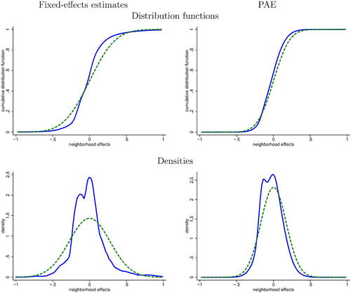
Fig. 1 Distribution of neighborhood effects

NOTE: In the left graphs, we show the distribution of fixed-effects estimates ${\widehat{\mu }}_c$ (solid) and its normal fit (dashed). In the right graphs, we show the posterior distribution of μ_c (solid) and the prior distribution (dashed). The distribution functions are shown in the top panel, the implied densities are shown in the bottom panel. Calculations are based on statistics available on the Equality of Opportunity website.

We next turn to data generating processes where α_i is not normal, drawn from a skewed Beta distribution. We find that the model-based estimator is substantially biased in this case. The nonparametric deconvolution estimator has smallest bias when errors are normally distributed, but it is heavily biased when errors are nonnormal. By contrast, although it has no consistency guarantees in these settings, the PAE tends to perform comparatively well in all situations, for bias and variance (see Appendix Figure S2).

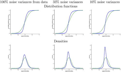
Fig. 2 Simulated data with log-normal μ_c

NOTE: Simulation with μ_c log-normal and ${\overline{\epsilon }}_c$ normal. The posterior distribution is shown in solid, the prior distribution is shown in dashed. The distribution functions are shown in the top panel, the implied densities are shown in the bottom panel. The left graphs correspond to the noise variances ${\widehat{s}}_c^2$ of the data, the middle ones correspond to the noise variances divided by 3, and the right graphs correspond to the noise variances divided by 10.

Overall, the simulations complement our theory by highlighting that, beyond specification error, other sources of estimation error matter in practice. Under correct specification of the reference distribution, the model-based estimator should be preferred. At the same time, our results suggest that, at least in the particular settings we focus on, the performance of the PAE appears less sensitive to misspecification than those of the model-based and nonparametric deconvolution estimators. Moreover, we find that the robustness gains provided by the PAE depend on the signal-to-noise ratio and the informativeness of the posterior conditioning. We provide details on the simulations in Appendix S4.

4.2 Neighborhood Effects

In this subsection and the next, we revisit two applications of models with latent variables. In our first illustration, we focus on a model of neighborhood effects following Chetty and Hendren (2018), using data for the US that these authors made public. In our second illustration, we study a permanent-transitory model of income dynamics (Hall and Mishkin 1982; Blundell et al. 2008) using the PSID. In both cases, we rely on a normal reference specification and assess how and by how much the posterior conditioning informs the estimates of the parameters of interest.

Here we start with estimates of neighborhood (or “place”) effects reported in Chetty and Hendren (2018, CH hereafter). Those were obtained using individuals who moved between different commuting zones at different ages. The outcome variable that we focus on is the causal estimate of the income rank at age 26 of a child whose parents are at the 25 percentile of the income distribution. This is CH’s preferred measure of place effect.

CH report an estimate of the variance of neighborhood effects, corrected for noise. In addition, they report individual predictors. Here we are interested in documenting the entire distribution of place effects. To do so, we consider the model ${\widehat{\mu }}_c={\mu }_c+{\overline{\epsilon }}_c$, for each commuting zone c, where ${\widehat{\mu }}_c$ is a neighborhood-specific fixed-effects reported by CH, μ_c is the true effect of neighborhood c, and ${\overline{\epsilon }}_c$ is additive estimation noise. CH also report estimates ${\widehat{s}}_c^2$ of the variances of ${\overline{\epsilon }}_c$ for every c. When weighted by population, the fixed-effects estimates ${\widehat{\mu }}_c$ have mean zero. We treat neighborhoods as independent observations. The statistics we use for calculations are available at: https://opportunityinsights.org/paper/neighborhoodsii/. Given the aggregate data at hand, we necessarily need to assume that estimates ${\widehat{\mu }}_c$ are independent across neighborhoods c, although this might be restrictive in this setting.

We first estimate the variance of place effects μ_c, following CH. We trim the top 1% percentile of ${\widehat{s}}_c^2$, and weigh all results by population weights. While this differs slightly from CH’s approach, which is based on $1/{\widehat{s}}_c^2$ precision weights and no trimming, we replicated the analysis using precision weights in the un-trimmed sample and found similar results. We have information about place effects in C = 590 commuting zones c in our sample, compared to 595 in the sample without trimming. We estimate a sizable variance of neighborhood fixed-effects: $\text{var}({\widehat{\mu }}_c)=0.077$. In turn, the mean of ${\widehat{s}}_c^2$ weighted by population is ${\widehat{s}}_{\overline{\epsilon }}^2=0.047$. Given those, we estimate the variance of place effects as ${\widehat{s}}_{\mu }^2=\text{var}({\widehat{\mu }}_c)-{\widehat{s}}_{\overline{\epsilon }}^2=0.030$. In this setting, the shrinkage factor ${\widehat{\rho }}_c={\widehat{s}}_{\mu }^2/({\widehat{s}}_{\mu }^2+{\widehat{s}}_c^2)$ exhibits substantial heterogeneity across commuting zones. Indeed, the mean of ${\widehat{\rho }}_c$ is 0.62, and its 10% and 90% percentiles are 0.21 and 0.93, respectively.

We use a normal with zero mean and variance ${\widehat{s}}_{\mu }^2$ as a prior for μ_c. Then, we estimate the distribution function of neighborhood effects ${\mu }_c$ using the PAE given by (5); that is,$${\widehat{F}}_{\mu }^{\mathrm{P}}(a)=\frac{1}{\sum _{c=1}^C{\pi }_c}\sum _{c=1}^C{\pi }_c\Phi \left(\frac{a-{\widehat{\rho }}_c{\widehat{\mu }}_c}{{\widehat{s}}_{\mu }\sqrt{1-{\widehat{\rho }}_c}}\right),$$where π_c are population weights. In addition, in order to ease the visualization of the results, we will also report estimates of densities, which are the derivatives of the PAE of distribution functions. Note that the density of μ at a can be approximated for arbitrarily small h > 0 by the expectation of $\mathbf{1}\left\{\right|\mu -a|/h\}/2h$. Taking the limit of the corresponding PAE as h tends to zero gives the derivative of ${\widehat{F}}_{\mu }^{\mathrm{P}}$ at a. We thus expect derivatives of PAE of distribution functions to enjoy similar minimum-worst-case specification error properties as PAE, but we do not formalize the required assumptions here.

In the top panel of Figure 1, we report several estimates of distribution functions. In the bottom panel, we report the corresponding density estimates. In the left graphs, we show nonparametric kernel estimates of the distribution function (respectively, density) of the fixed-effects ${\widehat{\mu }}_c$, weighted by population (in solid), together with the best-fitting normal (in dashed). The graphs show substantial nonnormality of the fixed-effects estimates. In particular, the large variance appears to be driven by some large positive and negative estimates ${\widehat{\mu }}_c$. In the right graphs, we report the PAE ${\widehat{F}}_{\mu }^{\mathrm{P}}$ of the distribution function of true place effects μ_c, with the associated density (in solid). In addition, we show the normal prior, with zero mean and variance ${\widehat{s}}_{\mu }^2$ (in dashed). The posterior distribution of neighborhood effects differs from the normal prior, although the two estimators have the same variance by construction. In comparison, neighborhood-specific EB estimates have a substantially lower dispersion. In appendix (Figure S5, supplementary material), we report an estimate of their distribution function ${\widehat{F}}_{\mu }^{\text{PM}}$ and associated density. While ${\widehat{s}}_{\mu }^2=0.030$ and the variance associated with ${\widehat{F}}_{\mu }^{\mathrm{P}}$ is 0.030, the variance of the EB estimates is only 0.010. In addition, a specification test that compares model-based estimator and PAE, which we described in Appendix S5 (supplementary material), suggests that these differences are statistically significant. Indeed, assuming independence across commuting zones, we obtain p-values below 0.01 at all deciles except the bottom two.

To assess how likely it is that the posterior estimator approximates the shape of the distribution of true neighborhood effects, we next perform two different exercises, based on a simulation and on numerical calculations motivated by our theory. We start with a Monte Carlo simulation, where μ_c, for $c=1,\dots ,C_{\text{sim}}$, are log-normally distributed with zero mean and variance ${\widehat{s}}_{\mu }^2$, and ${\overline{\epsilon }}_c$ are normally distributed independent of μ_c with zero mean. We consider three scenarios for the noise variances ${\widehat{s}}_c^2$: the estimates from CH, one-third of those values, and one-tenth of those values. In this exercise, we again weigh by population. We show the results for $C_{\text{sim}}=100,000$ simulated neighborhoods. In the left graphs of Figure 2, we see that, when the noise variances are the ones from the data, the posterior density is more skewed than the normal, yet the posterior shape is quite different from the true log-normal distribution of μ_c. When reducing the noise variances in the middle and right graphs, the posterior distribution function and density estimates get closer to the log-normal ones. In the right graphs, where the shrinkage factor is 0.90 on average (as opposed to 0.62 in the data), the posterior distribution function and density approximate the highly nonnormal shape of the true distribution of neighborhood effects very well.

We next turn to our posterior informativeness measure, which is given by Equation (21)(21) $$R^2=1-\frac{2T\left(\frac{a-{\widehat{\mu }}_{\alpha }}{{\widehat{s}}_{\alpha }},\sqrt{\frac{1-\widehat{\rho }}{1+\widehat{\rho }}}\right)}{\Phi \left(\frac{a-{\widehat{\mu }}_{\alpha }}{{\widehat{s}}_{\alpha }}\right)\left[1-\Phi \left(\frac{a-{\widehat{\mu }}_{\alpha }}{{\widehat{s}}_{\alpha }}\right)\right]}.$$(21) . Note the R² coefficient varies along the distribution. We find that the weighted average R² across values of a is 28%, where we weigh across cutoff values a by the reference distribution for α. This value is consistent with the message of Figure 2, since it suggests that, while the posterior conditioning informs the shape of the distribution of neighborhood effects, the signal-to-noise ratio is not high enough to be confident about the exact shape.

Last, we perform two additional exercises as robustness checks. First, we incorporate the mean income ${\overline{y}}_c$ of permanent residents in county c at the 25% percentile as a covariate. CH rely on information on permanent residents’ income to improve the accuracy of individual predictions. Here, we use it to refine the reference distribution and to improve the estimation of the distribution of neighborhood effects. Specifically, our reference model for μ_c is then a correlated random-effects specification, where the mean depends on ${\overline{y}}_c$ linearly. Appendix (Figure S6, supplementary material) shows small differences with our baseline estimates. Second, we re-do our main analysis at the county level, instead of the commuting zone level. In that case, the signal-to-noise ratio is lower, our posterior informativeness R² measure is 17% on average, and the appendix (Figure S7, supplementary material) shows that the normal prior and the posterior distributions are closer to each other than in the case of commuting zones.

4.3 Income Dynamics

In this subsection, we consider the following permanent-transitory model of household log-income:$$\begin{array}{c}{Y}_{it}={\eta }_{it}+{\epsilon }_{it},\mathrm{\hspace{1em}}\mathrm{\hspace{1em}}{\eta }_{it}={\eta }_{i,t-1}+V_{it},\\ i=1,\dots ,n,\hspace{1em}t=1,\dots ,T,\end{array}$$where ${\epsilon }_{it}$ and V_it are independent at all lags and leads, and independent of ${\eta }_{i0}$. This process is commonly used as an input for life-cycle consumption/savings models. Researchers often estimate covariances in a first step using minimum distance, and then impose a normality assumption for further analysis. However, there is increasing evidence that income components are not normally distributed. Instead of using a more flexible model—as has been done by Carlton and Hall (1978) and a large subsequent literature—here we compute PAEs. The advantages of this approach are that no additional assumptions are needed, and that implementation is straightforward.

We focus on six recent waves of the PSID 1999–2009 (every other year), see Blundell et al. (2016) for a description of the data. We use the same sample selection as in Arellano et al. (2017), and work with a balanced panel of n = 792 households over T = 6 periods. Y_it are residuals of log total pre-tax household labor earnings on a set of demographics, which include cohort interacted with education categories for both household members, race, state, and large-city dummies, a family size indicator, number of kids, a dummy for income recipient other than husband and wife, and a dummy for kids out of the household. Our aim is to estimate the distributions of η_it and ${\epsilon }_{it}$. To do so, we compare normal model-based estimates with posterior estimates, by plotting distribution functions as well as the implied densities. The model’s structure is similar to that of the fixed-effects model (1), and analytical expressions for posterior estimators are easy to derive.

In the left graphs of Figure 3, we show the distribution of the permanent component η_it. In the right graphs, we show the distribution of the transitory component ${\epsilon }_{it}$. We show PAE in solid, and model-based estimators in dashed. In the top panel we report estimates of distribution functions, and in the bottom panel we report the implied density estimates. The estimates show mild deviation from Gaussianity for the permanent component, and stronger evidence of non-Gaussianity for the transitory component. In particular, the latter shows excess kurtosis (i.e., “peakedness”) relative to the normal.

Fig. 3 Distribution of income components

NOTE: The top panel shows PAE estimates of distribution functions (in solid), and model-based estimates (in dashed), and the bottom panel shows the associated density estimates. The left graphs correspond to the permanent income component η_it, the right graphs to the transitory income component ${\epsilon }_{it}$. Sample from the PSID, 1999-2009.

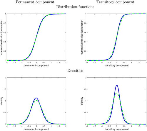
Several articles have already documented the presence of excess kurtosis in income components, particularly in transitory innovations, using parametric or semi-parametric methods. The estimates in Figure 3 share some qualitative similarities with recent findings in the literature. For example, the estimates of a flexible nonnormal and nonlinear model in Arellano et al. (2017, Figure 3) are quite similar to the PAE estimates in Figure 3 for permanent components. At the same time, their estimates of the distribution of transitory components show substantially more pronounced non-Gaussianity and excess kurtosis relative to PAE. This finding is in agreement with our posterior informativeness measure R², which is 12% on average along the distribution for the permanent component, and 8% on average for the transitory component. This degree of informativeness suggests that posterior estimates may suffer from substantial specification error when the reference distribution is misspecified.

Overall, these empirical illustrations give two examples where, starting from a normal prior, the posterior conditioning is informative about the true unknown distributions. In both settings, PAE are not normal. Yet, as indicated by the R² values we report, the signal-to-noise ratios are not high enough to be certain about the exact shapes of the distributions of interest, thus motivating further analyses using nonnormal specifications. PAE should be useful in other environments where model (1) and its extensions are widely used, for example in teacher value-added applications, where the signal-to-noise ratio is driven by the number of observations per teacher. Moreover, PAE are also applicable to other—nonlinear—econometric models, as we describe in the next section.

5 Complements and Extensions

In this section, we outline several complements and extensions that we analyze in detail in the appendix.

5.1 PAE in Other Models

PAE are applicable to a variety of settings. In many econometric models, semi-parametric estimators—that is, robust to distributional assumptions on unobservables—of β parameters are available; see Powell (1994) for examples. In such models, PAE provide estimators of average effects that enjoy robustness properties when parametric assumptions are violated. In Appendix S6, we study static binary and ordered choice models, censored regression models, and panel data binary choice models. We also show how the White (1980) formula for robust standard errors in linear regression can be interpreted as a PAE.

5.2 Confidence Intervals and Specification Test

Under correct specification of the reference model, it is easy to derive the asymptotic distributions of ${\widehat{\delta }}^{\mathrm{M}}$ and ${\widehat{\delta }}^{\mathrm{P}}$ using standard arguments. Moreover, under local misspecification, confidence intervals that account for both model uncertainty and sampling uncertainty can be constructed following Armstrong and Kolesár (2018) and Bonhomme and Weidner (2018). However, such confidence intervals require the researcher to set a value for the degree of misspecification ϵ. In Appendix S5 (supplementary material), we provide details on confidence intervals calculations. In addition, we explain how to construct a specification test of the reference model based on the difference ${\widehat{\delta }}^{\mathrm{P}}-{\widehat{\delta }}^{\mathrm{M}}$.

5.3 Robustness in Prediction

In applications such as the fixed-effects model (1) of teacher quality, researchers are often interested in predicting the quality α_i of teacher i. Although our focus in this article is on the estimation of population averages, it is interesting to see how different predictors perform under misspecification of the reference distribution. It is well known that EB estimators minimize mean squared prediction error when the normal reference model is correctly specified. However, when normality fails, the best predictor is a different posterior mean, which does not generally coincide with the EB estimate based on a normal prior. Intuitively, conditioning on nonlinear functions of the data may improve prediction accuracy.

In Appendix S3 (supplementary material), we use our framework—applied to worst-case mean squared prediction error instead of worst-case specification error of a sample average—to provide results on the robustness of EB estimators in the presence of misspecification. We show that EB estimators have minimum worst-case mean squared prediction error, up to smaller-order terms, under local deviations from normality. In addition, we derive a fixed-ϵ, nonlocal risk bound in the spirit of Theorem 3.

6 Conclusion

Posterior averages are commonly used to predict individual parameters, such as teacher quality or neighborhood effects, and they play a central role in Bayesian and EB approaches. In this article, we have provided a frequentist justification for posterior conditioning when the goal of the researcher is to estimate a population average quantity. We have shown that PAEs have minimum worst-case specification error under various forms of misspecification of parametric assumptions. PAE are simple to implement, and our analysis provides a rationale for reporting them in applications alongside other parametric and semi-parametric estimators, as well as a simple way to assess the informativeness of the posterior conditioning. As an example, Arnold et al. (2020) recently reported PAE to document judge heterogeneity in the context of bail decisions. While we have used a linear fixed-effects model as a running example due to its popularity, there are other possible applications, some of which we discuss in the appendix.

Supplementary Materials

The supplementary material contains an appendix with proofs, simulations, and extensions, as well as codes for replication.

Acknowledgments

We thank to two anonymous referees, Manuel Arellano, Tim Armstrong, Raj Chetty, Tim Christensen, Nathan Hendren, Peter Hull, Max Kasy, Derek Neal, Jesse Shapiro, Xiaoxia Shi, Danny Yagan, and audiences at various places for comments.

Additional information

Funding

Bonhomme acknowledges support from the NSF, Grant SES-1658920. Weidner acknowledges support from the Economic and Social Research Council through the ESRC Centre for Microdata Methods and Practice grant RES-589-28-0001 and from the European Research Council grants ERC-2014-CoG-646917-ROMIA and ERC-2018-CoG-819086-PANEDA.

References

- Abadie, A., and Kasy, M. (2018), “The Risk of Machine Learning,” Review of Economics and Statistics, to appear.
- Andrews, I., Gentzkow, M., and Shapiro, J. M. (2017), “Measuring the Sensitivity of Parameter Estimates to Estimation Moments,” Quarterly Journal of Economics, 132, 1553–1592. DOI: 10.1093/qje/qjx023.
- Andrews, I., Gentzkow, M., and Shapiro, J. M. (2020), “On the Informativeness of Descriptive Statistics for Structural Estimates,” Econometrica, 88, 2231–2258. DOI: 10.3982/ECTA16768.
- Angrist, J. D., Hull, P. D., Pathak, P. A., and Walters, C. R. (2017), “Leveraging Lotteries for School Value-Added: Testing and Estimation,” Quarterly Journal of Economics, 132, 871–919. DOI: 10.1093/qje/qjx001.
- Arellano, M., Blundell, R., and Bonhomme, S. (2017), “Earnings and Consumption Dynamics: A Nonlinear Panel Data Framework,” Econometrica, 85, 693–734. DOI: 10.3982/ECTA13795.
- Arellano, M., and Bonhomme, S. (2009), “Robust Priors in Nonlinear Panel Data Models,” Econometrica, 77, 489–536.
- Armstrong, T. B., and Kolesár, M. (2018), “Sensitivity Analysis Using Approximate Moment Condition Models,” arXiv preprint arXiv:1808.07387.
- Arnold, D., W. S. Dobbie, and P. Hull (2020), “Measuring Racial Discrimination in Bail Decisions,” (No. w26999). National Bureau of Economic Research.
- Berger, J. (1980), Statistical Decision Theory: Foundations, Concepts, and Methods, New York: Springer-Verlag.
- Bickel, P. J., Klaassen, C. A. J., Ritov, Y., and Wellner, J. A. (1993), Efficient and Adaptive Inference in Semiparametric Models, Baltimore: Johns Hopkins University Press.
- Blundell, R., Pistaferri, L., and Preston, I. (2008): “Consumption Inequality and Partial Insurance,” American Economic Review, 98, 1887–1921. DOI: 10.1257/aer.98.5.1887.
- Blundell, R., Pistaferri, L., and Saporta-Eksten, I. (2016), “Consumption Smoothing and Family Labor Supply,” American Economic Review, 106, 387–435. DOI: 10.1257/aer.20121549.
- Bonhomme, S., and Robin, J. M. (2010), “Generalized Nonparametric Deconvolution With an Application to Earnings Dynamics,” Review of Economic Studies, 77, 491–533. DOI: 10.1111/j.1467-937X.2009.00577.x.
- Bonhomme, S., and Weidner, M. (2018), “Minimizing sensitivity to model misspecification,” arXiv:1807.02161.
- Carlton, D. W., and Hall, R. E. (1978), “The Distribution of Permanent Income,” in Income Distribution and Economic Inequality, New York: Halsted.
- Chetty, R., Friedman, J. N., and Rockoff, J. E. (2014), “Measuring the Impacts of Teachers I: Evaluating Bias in Teacher Value-Added Estimates,” American Economic Review, 104, 2593–2632. DOI: 10.1257/aer.104.9.2593.
- Chetty, R., and Hendren, N. (2018), “The Impacts of Neighborhoods on Intergenerational Mobility: County-Level Estimates,” Quarterly Journal of Economics, 133, 1163–1228.
- Christensen, T., and Connault, B. (2019), “Counterfactual Sensitivity and Robustness,” unpublished manuscript.
- Cressie, N., and Read, T. R. C. (1984), “Multinomial Goodness-of-Fit Tests,” Journal of the Royal Statistical Society, Series B, 46, 440–464. DOI: 10.1111/j.2517-6161.1984.tb01318.x.
- Delaigle, A., Hall, P., and Meister, A. (2008), “On Deconvolution With Repeated Measurements,” Annals of Statistics, 36, 665–685.
- Dobbie, W., and Fryer, R. G. Jr(2013), “Getting Beneath the Veil of Effective Schools: Evidence from New York City,” American Economic Journal: Applied Economics, 5, 28–60. DOI: 10.1257/app.5.4.28.
- Efron, B. (2012), Large-Scale Inference: Empirical Bayes Methods for Estimation, Testing, and Prediction, Vol. 1. Cambridge: Cambridge University Press.
- Efron, B., and Morris, C. (1973), “Stein’s Estimation Rule and its Competitors – An Empirical Bayes Approach,” Journal of the American Statistical Association, 68, 117–130.
- Fessler, P., and Kasy, M. (2018), “How to Use Economic Theory to Improve Estimators,” to appear in the Review of Economics and Statistics. DOI: 10.1162/rest_a_00795.
- Finkelstein, A., Gentzkow, M., Hull, P., and Williams, H. (2017), “Adjusting Risk Adjustment – Accounting for Variation in Diagnostic Intensity,” New England Journal of Medicine, 376, 608–610. DOI: 10.1056/NEJMp1613238.
- Geweke, J., and Keane, M. (2000), “An Empirical Analysis of Earnings Dynamics Among Men in the PSID: 1968-1989,” Journal of Econometrics, 96, 293–356. DOI: 10.1016/S0304-4076(99)00063-9.
- Guvenen, F., Karahan, F., Ozcan, S., and Song, J. (2016), “What Do Data on Millions of U.S. Workers Reveal about Life-Cycle Earnings Risk?” Econometrica.
- Hall, R., and Mishkin, F. (1982), “The Sensitivity of Consumption to Transitory Income: Estimates from Panel Data of Households,” Econometrica, 50, 261–81. DOI: 10.2307/1912638.
- Hansen, B. E. (2016), “Efficient Shrinkage in Parametric Models,” Journal of Econometrics, 190, 115–132. DOI: 10.1016/j.jeconom.2015.09.003.
- Hirano, K. (2002), “Semiparametric Bayesian Inference in Autoregressive Panel Data Models,” Econometrica, 70, 781–799. DOI: 10.1111/1468-0262.00305.
- Huber, P. J., and Ronchetti, E. M. (2009), Robust Statistics, 2nd ed., Hoboken, NJ: Wiley.
- Hull, P. (2018), “Estimating Hospital Quality with Quasi-Experimental Data,” unpublished manuscript.
- Ignatiadis, N., and S. Wager (2019), “Bias-Aware Confidence Intervals for Empirical Bayes Analysis,” arXiv:1902.02774.
- James, W., and Stein, C. (1961), “Estimation with Quadratic Loss,” in Proc. Fourth Berkeley Symp. Math. Statist. Prob., 1, 361–379. Univ. of California Press.
- Jochmans, K., and Weidner, M. (2018), “Inference on a Distribution From Noisy Draws,” arXiv:1803.04991.
- Kane, T. J., and Staiger, D. O. (2008), “Estimating Teacher Impacts on Student Achievement: An Experimental Evaluation”, National Bureau of Economic Research (No. w14607).
- Kitamura, Y., Otsu, T., and Evdokimov, K. (2013), “Robustness, Infinitesimal Neighborhoods, and Moment Restrictions,” Econometrica, 81, 1185–1201.
- Koenker, R., and Mizera, I. (2014), “Convex Optimization, Shape Constraints, Compound Decisions, and Empirical Bayes Rules,” Journal of the American Statistical Association, 109, 674–685. DOI: 10.1080/01621459.2013.869224.
- Kotlarski, I. (1967), “On Characterizing the Gamma and the Normal Distribution,” Pacific Journal of Mathematics, 20, 69–76. DOI: 10.2140/pjm.1967.20.69.
- Li, T., and Vuong, Q. (1998), “Nonparametric Estimation of the Measurement Error Model Using Multiple Indicators,” Journal of Multivariate Analysis, 65, 139–165. DOI: 10.1006/jmva.1998.1741.
- Morris, C. N. (1983), “Parametric Empirical Bayes Inference: Theory and Applications,” Journal of the American Statistical Association, 78, 47–55. DOI: 10.1080/01621459.1983.10477920.
- Owen, D. B. (1956), “Tables for Computing Bivariate Normal Probabilities,” The Annals of Mathematical Statistics, 27, 1075–1090. DOI: 10.1214/aoms/1177728074.
- Powell, J. L. (1994), “Estimation of Semiparametric Models,” Handbook of Econometrics, 4, 2443–2521.
- Stefanski, L. A., and Carroll, R. J. (1990), “Deconvolving Kernel Density Estimators,” Statistics, 21, 169–184. DOI: 10.1080/02331889008802238.
- White, H. (1980), “A Heteroskedasticity-Consistent Covariance Matrix Estimator and a Direct Test for Heteroskedasticity,” Econometrica: Journal of the Econometric Society, 817–838. DOI: 10.2307/1912934.