Local Composite Quantile Regression for Regression Discontinuity

Abstract

We introduce the local composite quantile regression (LCQR) to causal inference in regression discontinuity (RD) designs. Kai, Li and Zou study the efficiency property of LCQR, while we show that its nice boundary performance translates to accurate estimation of treatment effects in RD under a variety of data generating processes. Moreover, we propose a bias-corrected and standard error-adjusted t-test for inference, which leads to confidence intervals with good coverage probabilities. A bandwidth selector is also discussed. For illustration, we conduct a simulation study and revisit a classic example from Lee. A companion R package rdcqr is developed.

Keywords:

• Local composite quantile regression
• Regression discontinuity
• Treatment effect

1 Introduction

Over the past few decades, regression discontinuity (RD) has become a popular quasi-experimental method to identify the local average treatment effect. In its simplest form, the sharp RD design, a unit i receives treatment if and only if an underlying variable X_i attains a prespecified cutoff. Under some smoothness assumptions, units in a small neighborhood of the cutoff share similar characteristics so that the difference between the outcomes above and below the cutoff can be interpreted as the local average treatment effect. For recent discussions of the literature and background references, see, for example, Cattaneo, Idrobo, and Titiunik (2019, 2020).

Central to a large portion of the empirical and theoretical work on RD is the use of local linear regression (LLR; see Fan and Gijbels 1996), while the goal of this article is to introduce another nonparametric smoother to the estimation and inference in sharp as well as fuzzy RD designs. Although LLR is the best linear smoother, it is possible to use an alternative estimator in RD if we consider the larger class of nonlinear smoothers. One such example is the local composite quantile regression (LCQR) method in Kai, Li, and Zou (2010), who show that LCQR can have some efficiency gain against LLR when data are nonnormal. The literature related to LCQR is growing. Several recent examples include Kai, Li, and Zou (2011), Zhao and Xiao (2014), Li and Li (2016), and Huang and Lin (2021), although none of these studies focuses on RD. To use LCQR, the researcher chooses a finite number of quantile positions, say 5, and uses a local polynomial to estimate the quantile (the intercept) at each of the 5 quantile positions. Averaging the 5 quantile estimates gives an estimate for the conditional mean, whose values above and below the prespecified cutoff are the key components in sharp and fuzzy RD designs.

Our article makes the following contributions to the large and growing literature on RD. First, we introduce the LCQR method to sharp and fuzzy RD designs. Numerical evidence for the efficiency gain of using LCQR instead of LLR in RD is also provided. Second, similar to the robust t-test in Calonico, Cattaneo, and Titiunik (2014) for conducting inference on causal effects, we propose a t-test that adjusts both the bias and the standard error of the LCQR estimator, and the resulting confidence intervals are shown to have good coverage probabilities. Third, we further discuss a new bandwidth selector that is based on an adjusted mean squared error (MSE). As a byproduct of our research, we also develop an R package rdcqr that implements the LCQR method in this article. The rdcqr package can be downloaded from https://github.com/xhuang20/rdcqr.

The rest of the article unfolds as follows. Section 2 sets up the notation for RD designs and introduces the LCQR method. Section 3 presents the bias correction and standard error adjustment for inference on the boundary. Section 4 briefly discusses several extensions, such as allowing for covariates and kink RD designs. Section 5 presents a simulation experiment. An empirical illustration of LCQR for RD is provided in Section 6 using the data from Lee (2008). Section 7 concludes. The online supplement contains all technical details and proofs, as well as additional figures and tables.

2 RD and Local Composite Quantile Regression

We introduce the notation for RD and the application of LCQR in RD in this section.

2.1 RD: Setup and Notation

Consider the triplet $(Y_i,X_i,T_i),i=1,\dots ,n$ in a standard RD setup that nests both the sharp and fuzzy RD designs. Y_i is the observed outcome for individual i, X_i is the variable that determines the assignment of treatment, and T_i equals 1 if individual i receives treatment and 0 otherwise. For individual i to receive treatment, a threshold value for X_i is set. Without loss of generality, we assume the threshold is 0, and the treatment assignment rule becomes that individual i is assigned to the treatment group if $X_i\ge 0$. Throughout the article, the signs + and – will be used to denote data or quantities associated with $X_i\ge 0$ and $X_i<0$, respectively.

We use a general nonparametric model to describe the relationship between Y_i and X_i (1) $$Y_{+,i}=m_{Y_{+}}(X_{+,i})+{\sigma }_{{ϵ}_{Y_{+}}}(X_{+,i}){ϵ}_{Y_{+},i},$$(1) (2) $$Y_{-,i}=m_{Y_{-}}(X_{-,i})+{\sigma }_{{ϵ}_{Y_{-}}}(X_{-,i}){ϵ}_{Y_{-},i},$$(2) where $m_{Y_{+}},m_{Y_{-}},{\sigma }_{{ϵ}_{Y_{+}}},{\sigma }_{{ϵ}_{Y_{-}}},{ϵ}_{Y_{+}}$, and ${ϵ}_{Y_{-}}$ are the conditional mean functions, conditional standard deviation functions, and error terms with unit variance, respectively.

In a sharp RD design, whether individual i receives treatment is determined by whether $X_i\ge 0$, so $T_i=I\{X_i\ge 0\}$. One is interested in measuring the average treatment effect at the threshold 0(3) $${\tau }_{\text{sharp}}=m_{Y_{+}}(0)-m_{Y_{-}}(0),$$(3) where(4) $$m_{Y_{+}}(0)=\underset{x_{+}\downarrow 0}{\lim }{m}_{Y_{+}}(x_{+})\mathrm{ }\text{and}\mathrm{ }{m}_{Y_{-}}(0)=\underset{x_{-}\uparrow 0}{\lim }{m}_{Y_{-}}(x_{-}).$$(4)

A t-statistic for testing a hypothesized treatment effect τ₀ reads(5) $$t_{\text{sharp}}=\frac{{\widehat{\tau }}_{\text{sharp}}-{\tau }_0}{\sqrt{\text{var}({\widehat{\tau }}_{\text{sharp}})}},$$(5) where, under the iid assumption, we have(6) $$\begin{array}{c}{\widehat{\tau }}_{\text{sharp}}={\widehat{m}}_{Y_{+}}(0)-{\widehat{m}}_{Y_{-}}(0),\\ \text{var}({\widehat{\tau }}_{\text{sharp}})=\text{var}({\widehat{m}}_{Y_{+}}(0))+\text{var}({\widehat{m}}_{Y_{-}}(0)).\end{array}$$(6)

In a fuzzy RD design, the treatment assignment rule remains the same, but T_i is not necessarily equal to 1 when $X_i\ge 0$ or 0 when $X_i<0$. It is customary to use a nonparametric function to describe the probability of receiving treatment(7) $$T_{+,i}=m_{T_{+}}(X_{+,i})+{\sigma }_{{ϵ}_{T_{+}}}(X_{+,i}){ϵ}_{T_{+},i},$$(7) (8) $$T_{-,i}=m_{T_{-}}(X_{-,i})+{\sigma }_{{ϵ}_{T_{-}}}(X_{-,i}){ϵ}_{T_{-},i}.$$(8)

The treatment effect measurement becomes(9) $${\tau }_{\text{fuzzy}}=\frac{m_{Y_{+}}(0)-m_{Y_{-}}(0)}{m_{T_{+}}(0)-m_{T_{-}}(0)},$$(9) where $m_{Y_{+}}(0),m_{Y_{-}}(0)$ are as defined in Equation (4)(4) $$m_{Y_{+}}(0)=\underset{x_{+}\downarrow 0}{\lim }{m}_{Y_{+}}(x_{+})\mathrm{ }\text{and}\mathrm{ }{m}_{Y_{-}}(0)=\underset{x_{-}\uparrow 0}{\lim }{m}_{Y_{-}}(x_{-}).$$(4) above, and similarly,(10) $$m_{T_{+}}(0)=\underset{x_{+}\downarrow 0}{\lim }{m}_{T_{+}}(x_{+})\mathrm{ }\text{and}\mathrm{ }{m}_{T_{-}}(0)=\underset{x_{-}\uparrow 0}{\lim }{m}_{T_{-}}(x_{-}).$$(10)

The corresponding t-statistic is given by(11) $$t_{\text{fuzzy}}=\frac{{\widehat{\tau }}_{\text{fuzzy}}-{\tau }_0}{\sqrt{\text{var}({\widehat{\tau }}_{\text{fuzzy}})}},$$(11) where(12) $${\widehat{\tau }}_{\text{fuzzy}}=\frac{{\widehat{m}}_{Y_{+}}(0)-{\widehat{m}}_{Y_{-}}(0)}{{\widehat{m}}_{T_{+}}(0)-{\widehat{m}}_{T_{-}}(0)},$$(12) and $\text{var}({\widehat{\tau }}_{\text{fuzzy}})$ depends on the variances and covariances of ${\widehat{m}}_{Y_{+}}(0),{\widehat{m}}_{Y_{-}}(0),{\widehat{m}}_{T_{+}}(0)$ and ${\widehat{m}}_{T_{-}}(0)$, which we provide in the online supplement (see (A.16) in Section S.2, supplementary material) to conserve space.

To conduct the t-test, we thus need nonparametric estimates for all quantities in Equations (6)(6) $$\begin{array}{c}{\widehat{\tau }}_{\text{sharp}}={\widehat{m}}_{Y_{+}}(0)-{\widehat{m}}_{Y_{-}}(0),\\ \text{var}({\widehat{\tau }}_{\text{sharp}})=\text{var}({\widehat{m}}_{Y_{+}}(0))+\text{var}({\widehat{m}}_{Y_{-}}(0)).\end{array}$$(6) and (12)(12) $${\widehat{\tau }}_{\text{fuzzy}}=\frac{{\widehat{m}}_{Y_{+}}(0)-{\widehat{m}}_{Y_{-}}(0)}{{\widehat{m}}_{T_{+}}(0)-{\widehat{m}}_{T_{-}}(0)},$$(12) at the boundary point 0.

2.2 Local Composite Quantile Regression

LLR is the leading method to estimate quantities in Equations (6)(6) $$\begin{array}{c}{\widehat{\tau }}_{\text{sharp}}={\widehat{m}}_{Y_{+}}(0)-{\widehat{m}}_{Y_{-}}(0),\\ \text{var}({\widehat{\tau }}_{\text{sharp}})=\text{var}({\widehat{m}}_{Y_{+}}(0))+\text{var}({\widehat{m}}_{Y_{-}}(0)).\end{array}$$(6) and (12)(12) $${\widehat{\tau }}_{\text{fuzzy}}=\frac{{\widehat{m}}_{Y_{+}}(0)-{\widehat{m}}_{Y_{-}}(0)}{{\widehat{m}}_{T_{+}}(0)-{\widehat{m}}_{T_{-}}(0)},$$(12) . LCQR is introduced in Kai, Li, and Zou (2010) as an alternative to the LLR method due to its potential efficiency gains with nonnormal errors. The probable advantage under non-normality is the key reason we propose to use LCQR in RD as normality can be easily violated in practice.

The same LCQR method can be applied to Equations (1)(1) $$Y_{+,i}=m_{Y_{+}}(X_{+,i})+{\sigma }_{{ϵ}_{Y_{+}}}(X_{+,i}){ϵ}_{Y_{+},i},$$(1) , (2)(2) $$Y_{-,i}=m_{Y_{-}}(X_{-,i})+{\sigma }_{{ϵ}_{Y_{-}}}(X_{-,i}){ϵ}_{Y_{-},i},$$(2) , (7)(7) $$T_{+,i}=m_{T_{+}}(X_{+,i})+{\sigma }_{{ϵ}_{T_{+}}}(X_{+,i}){ϵ}_{T_{+},i},$$(7) , and (8)(8) $$T_{-,i}=m_{T_{-}}(X_{-,i})+{\sigma }_{{ϵ}_{T_{-}}}(X_{-,i}){ϵ}_{T_{-},i}.$$(8) . Because of this similarity, we describe the LCQR method based on Equation (1)(1) $$Y_{+,i}=m_{Y_{+}}(X_{+,i})+{\sigma }_{{ϵ}_{Y_{+}}}(X_{+,i}){ϵ}_{Y_{+},i},$$(1) . For $k=1,\dots ,q$, let ${\tau }_k=k/(q+1)$ be the equally spaced q quantile positions and ${\rho }_{{\tau }_k}(r)={\tau }_{k}r-rI(r<0)$ be the q check loss functions in quantile regression. The loss function for LCQR at the point x is defined as follows:(13) $$\sum _{k=1}^q\sum _{i=1}^{n_{+}}{\rho }_{{\tau }_k}\left(Y_{+,i}-a_k-b(X_{+,i}-x)\right)K\left(\frac{X_{+,i}-x}{h_{Y+}}\right),$$(13) where a_k is the kth quantile estimand, b is a slope restricted to be the same across quantiles, $h_{Y+}$ is the bandwidth, and K is a kernel function. Here, we use the linear approximation to the conditional mean function in Equation (1)(1) $$Y_{+,i}=m_{Y_{+}}(X_{+,i})+{\sigma }_{{ϵ}_{Y_{+}}}(X_{+,i}){ϵ}_{Y_{+},i},$$(1) . Let $F_{Y|X}$ be the cumulative distribution function of Y given X so that $a_k=F_{Y|X=x}^{-1}({\tau }_k)$ is the kth quantile, and b is $m_{Y_{+}}^{(1)}(x)$, the first derivative of the conditional mean function at x. Using a single slope b allows us to combine information across quantiles, since a specification allowing for b_k in Equation (13)(13) $$\sum _{k=1}^q\sum _{i=1}^{n_{+}}{\rho }_{{\tau }_k}\left(Y_{+,i}-a_k-b(X_{+,i}-x)\right)K\left(\frac{X_{+,i}-x}{h_{Y+}}\right),$$(13) would be equivalent to estimating each quantile separately. Our point of interest in Equation (13)(13) $$\sum _{k=1}^q\sum _{i=1}^{n_{+}}{\rho }_{{\tau }_k}\left(Y_{+,i}-a_k-b(X_{+,i}-x)\right)K\left(\frac{X_{+,i}-x}{h_{Y+}}\right),$$(13) is x = 0.

The parameter q plays an important role here. Once q is chosen, there will be q quantiles corresponding to the q quantile positions τ_k . Since we use equally spaced quantile positions, the median will always be selected as the middle quantile if q is odd. For example, if q = 3, the quantile positions are $0.25,0.5,\text{and}0.75$. The goal is to spread the quantile positions on the interval (0, 1) so that LCQR can combine information in multiple quantiles. The value of q is decided by the researcher. Results in Kai, Li, and Zou (2010) and our discussion later on show that a small number such as 5, 7, or 9 may be adequate for many common nonnormal errors. It can be viewed as a hyperparameter and can be tuned.

Minimizing Equation (13)(13) $$\sum _{k=1}^q\sum _{i=1}^{n_{+}}{\rho }_{{\tau }_k}\left(Y_{+,i}-a_k-b(X_{+,i}-x)\right)K\left(\frac{X_{+,i}-x}{h_{Y+}}\right),$$(13) w.r.t. a_k and b yields $({\widehat{a}}_1,\dots ,{\widehat{a}}_q,\widehat{b})$. The LCQR estimator for $m_{Y+}(x)$ is defined as follows:(14) $${\widehat{m}}_{Y_{+}}(x)=\frac{1}{q}\sum _{k=1}^q{\widehat{a}}_k$$(14) and $\widehat{b}$ is the estimator for $m_{Y_{+}}^{(1)}(x)$, the first derivative of $m_{Y_{+}}(x)$. In a similar fashion, ${\widehat{m}}_{Y_{-}}(x),{\widehat{m}}_{T_{+}}(x)$, and ${\widehat{m}}_{T_{-}}(x)$ can be obtained at x = 0. The average in Equation (14)(14) $${\widehat{m}}_{Y_{+}}(x)=\frac{1}{q}\sum _{k=1}^q{\widehat{a}}_k$$(14) combines information across different quantile estimators. The hope is to possibly improve the relative efficiency of individual nonparametric quantile estimator to the nonparametric mean estimator based on LLR.

Kai, Li, and Zou (2010) discussed the asymptotic bias and variance of the LCQR estimator at an interior point x. The asymptotic properties at a boundary point x are discussed in Kai, Li, and Zou (2009). Given the results in Kai, Li, and Zou (2009), one can immediately implement the t-test for the sharp RD in Equation (5)(5) $$t_{\text{sharp}}=\frac{{\widehat{\tau }}_{\text{sharp}}-{\tau }_0}{\sqrt{\text{var}({\widehat{\tau }}_{\text{sharp}})}},$$(5) with bias correction if needed. To implement the t-test for the fuzzy RD in Equation (11)(11) $$t_{\text{fuzzy}}=\frac{{\widehat{\tau }}_{\text{fuzzy}}-{\tau }_0}{\sqrt{\text{var}({\widehat{\tau }}_{\text{fuzzy}})}},$$(11) , additional covariance expressions for Equation (12)(12) $${\widehat{\tau }}_{\text{fuzzy}}=\frac{{\widehat{m}}_{Y_{+}}(0)-{\widehat{m}}_{Y_{-}}(0)}{{\widehat{m}}_{T_{+}}(0)-{\widehat{m}}_{T_{-}}(0)},$$(12) need to be estimated and we provide these results in Lemma 3 in the online supplement. The asymptotic results for the bias and variance of ${\widehat{m}}_{Y_{+}}(x),{\widehat{m}}_{Y_{-}}(x),{\widehat{m}}_{T_{+}}(x)$, and ${\widehat{m}}_{T_{-}}(x)$ follow those in Kai, Li, and Zou (2009), and are given in Lemma 2 in the online supplement.

We make the following assumptions. Let c be a positive constant of supp(K).

Assumption 1.

$m_{Y_{+}}(·),m_{T_{+}}(·),m_{Y_{-}}(·)$, and $m_{T_{-}}(·)$ are at least three times continuously differentiable at x.

Assumption 2.

${\sigma }_{{ϵ}_{Y_{+}}}(·),{\sigma }_{{ϵ}_{T_{+}}}(·),{\sigma }_{{ϵ}_{Y_{-}}}(·)$, and ${\sigma }_{{ϵ}_{T_{-}}}(·)$ are right or left continuous and differentiable at x.

Assumption 3.

The kernel function K is bounded and symmetric.

Following Assumption 3, we define, for j = 0, 1, 2, $\cdots$,$$\begin{array}{c}{\mu }_{+,j}(c)={\int }_{-c}^{\infty }{u}^{j}K(u)du,\mathrm{\hspace{1em}}\mathrm{\hspace{1em}}{\nu }_{+,j}={\int }_{-c}^{\infty }{u}^j{K}^2(u)du,\\ {\mu }_{-,j}(c)={\int }_{-\infty }^c{u}^{j}K(u)du,\mathrm{\hspace{1em}}\mathrm{\hspace{1em}}{\nu }_{-,j}={\int }_{-\infty }^c{u}^j{K}^2(u)du.\end{array}$$

Assumption 4.

The marginal density $f_{X_{+}}(·)$ is right continuous, differentiable and positive at x = 0, and $f_{X_{-}}(·)$ is left continuous, differentiable and positive at x = 0.

Assumption 5.

All error distributions for ${ϵ}_{Y_{+}},{ϵ}_{T_{+}},{ϵ}_{Y_{-}}$, and ${ϵ}_{T_{-}}$ are symmetric and have positive density. All errors are i.i.d.

Assumption 6.

$h_{Y_{+}}\to 0,n_{+}{h}_{Y_{+}}\to \infty$, and $n_{+}{h}_{Y_{+}}^7\to 0$ as $n_{+}\to \infty$. The same condition also holds for $(n_{+},h_{T_{+}}),(n_{-},h_{Y_{-}})$, and $(n_{-},h_{T_{-}})$.

Assumptions 1 and 2 are used for Taylor series expansions in the proof. The bias expressions require only the second-order differentiability of the conditional mean function. Higher-order differentiability permits the study of small order terms in the expansion. The support of the kernel is assumed to be $(-\infty ,\infty )$ in Assumption 3. If the kernel has a bounded support such as $[-1,1]$, then we would have ${\mu }_{+,j}(c)={\int }_{-c}^1{u}^{j}K(u)du$. Similar changes can be made to the ν variables. The differentiability in Assumption 4 is also used for Taylor expansions in the proof, and we require the positivity of the density at the boundary as it appears in the denominator of the bias expression. The symmetric error distribution assumption in Assumption 5 helps remove an extra term in the bias. When the error distribution is asymmetric, this extra term can be removed during bias correction. In Assumption 6, $h_{Y_{+}}\to 0$ and $n_{+}{h}_{Y_{+}}\to \infty$ help establish the consistency of ${\widehat{m}}_{Y_{+}}$. The assumption $n_{+}{h}_{Y_{+}}^7\to 0$ is used to establish the asymptotic normality of the bias-corrected and s.e.-adjusted t-statistic. Assumption 6 translates to $h\to 0,nh\to \infty$, and $n{h}^7\to 0$ as $n\to \infty$ if we use a single bandwidth h for the data above and below the cutoff, and n is the total number of observations. Similar assumptions can be found in Calonico, Cattaneo, and Titiunik (2014) for LLR.

Next we provide two theorems on the LCQR estimator for sharp and fuzzy treatment effects defined in Equations (6)(6) $$\begin{array}{c}{\widehat{\tau }}_{\text{sharp}}={\widehat{m}}_{Y_{+}}(0)-{\widehat{m}}_{Y_{-}}(0),\\ \text{var}({\widehat{\tau }}_{\text{sharp}})=\text{var}({\widehat{m}}_{Y_{+}}(0))+\text{var}({\widehat{m}}_{Y_{-}}(0)).\end{array}$$(6) and (12)(12) $${\widehat{\tau }}_{\text{fuzzy}}=\frac{{\widehat{m}}_{Y_{+}}(0)-{\widehat{m}}_{Y_{-}}(0)}{{\widehat{m}}_{T_{+}}(0)-{\widehat{m}}_{T_{-}}(0)},$$(12) , respectively. Let X be the σ-field generated by all X_i .

Theorem 1.

Under Assumptions 1–6, as both $n_{+}$ and $n_{-}\to \infty$, we have(15) $$\begin{array}{c}\text{Bias}({\widehat{\tau }}_{\text{sharp}}|\mathbf{X})=\frac{1}{2}{a}_{Y_{+}}(c)m_{Y+}^{(2)}(0)h_{Y_{+}}^2-\frac{1}{2}{a}_{Y_{-}}(c)m_{Y-}^{(2)}(0)h_{Y_{-}}^2\\ \mathrm{\hspace{1em}}\mathrm{\hspace{1em}}+o_p(h_{Y_{+}}^2+h_{Y_{-}}^2),\end{array}$$(15) (16) $$\begin{array}{c}\text{var}({\widehat{\tau }}_{\text{sharp}}|\mathbf{X})=\frac{b_{Y_{+}}(c){\sigma }_{{ϵ}_{Y_{+}}}^2(0)}{n_{+}{h}_{Y_{+}}{f}_{X_{+}}(0)}+\frac{b_{Y_{-}}(c){\sigma }_{{ϵ}_{Y_{-}}}^2(0)}{n_{-}{h}_{Y_{-}}{f}_{X_{-}}(0)}\\ \mathrm{\hspace{1em}}\mathrm{\hspace{1em}}+o_p(\frac{1}{n_{+}{h}_{Y_{+}}}+\frac{1}{n_{-}{h}_{Y_{-}}}),\end{array}$$(16) where(17) $$a_{Y_{+}}(c)=a_{Y_{-}}(c)=\frac{{\mu }_{+,2}^2(c)-{\mu }_{+,1}(c){\mu }_{+,3}(c)}{{\mu }_{+,0}(c){\mu }_{+,2}(c)-{\mu }_{+,1}^2(c)},$$(17) (18) $$b_{Y_{+}}(c)=e_q^T{(S_{Y_{+}}^{-1}(c){\Sigma }_{Y_{+}}(c)S_{Y_{+}}^{-1}(c))}_{11}{e}_q/q^2,$$(18) (19) $$b_{Y_{-}}(c)=e_q^T{(S_{Y_{-}}^{-1}(c){\Sigma }_{Y_{-}}(c)S_{Y_{-}}^{-1}(c))}_{11}{e}_q/q^2,$$(19) and the matrices $S_{Y_{+}}(c),{\Sigma }_{Y_{+}}(c)$ and similarly, $S_{Y_{-}}(c),{\Sigma }_{Y_{-}}(c)$, are given in the online supplement (Section S.1, Equation (A.1)). e_q is the q-dimensional vector of ones.

Proof of Theorem 1 is a straightforward application of Theorem 2.1 in Kai, Li, and Zou (2009). As long as a symmetric kernel is used, the value of $a_{Y_{+}}(c)$ remains the same if kernel moments on the other side of the cutoff are used. Generally, we have $b_{Y_{+}}(c)\ne b_{Y_{-}}(c)$ unless error distributions on both sides of the cutoff are assumed to be the same.

When the bandwidths above and below the cutoff are assumed to be the same, Theorem 1 reduces to the following corollary.

Corollary 1.

Under Assumptions 1–6, if we further assume $h_{Y_{+}}=h_{Y_{-}}=h$, then we have(20) $$\begin{array}{c}\text{Bias}({\widehat{\tau }}_{\text{sharp}}|\mathbf{X})=\frac{1}{2}\left[a_{Y_{+}}(c)m_{Y+}^{(2)}(0)-a_{Y_{-}}(c)m_{Y-}^{(2)}(0)\right]h^2\\ \mathrm{\hspace{1em}}\mathrm{\hspace{1em}}+o_p(h^2),\end{array}$$(20) (21) $$\begin{array}{c}\text{var}({\widehat{\tau }}_{\text{sharp}}|\mathbf{X})=\frac{b_{Y_{+}}(c){\sigma }_{{ϵ}_{Y_{+}}}^2(0)}{n_{+}h{f}_{X_{+}}(0)}+\frac{b_{Y_{-}}(c){\sigma }_{{ϵ}_{Y_{-}}}^2(0)}{n_{-}h{f}_{X_{-}}(0)}\\ \mathrm{\hspace{1em}}\mathrm{\hspace{1em}}+o_p(\frac{1}{n_{+}h}+\frac{1}{n_{-}h}).\end{array}$$(21)

The asymptotic results for the fuzzy RD are similarly provided in the theorem below.

Theorem 2.

Under Assumptions 1–6, as both $n_{+}$ and $n_{-}\to \infty$, we have(22) $$\begin{array}{c}\text{Bias}({\widehat{\tau }}_{\text{fuzzy}}|\mathbf{X})\\ =\frac{1}{m_{T_{+}}(0)-m_{T_{-}}(0)}\left[\frac{1}{2}{a}_{Y_{+}}(c)m_{Y+}^{(2)}(0)h_{Y_{+}}^2-\frac{1}{2}{a}_{Y_{-}}(c)m_{Y-}^{(2)}(0)h_{Y_{-}}^2\right]\\ \hspace{1em}-\frac{m_{Y_{+}}(0)-m_{Y_{-}}(0)}{{\left[m_{T_{+}}(0)-m_{T_{-}}(0)\right]}^2}\left[\frac{1}{2}{a}_{T_{+}}(c)m_{T+}^{(2)}(0)h_{T_{+}}^2-\frac{1}{2}{a}_{T_{-}}(c)m_{T-}^{(2)}(0)h_{T_{-}}^2\right]\\ \hspace{1em}+o_p(h_{Y_{+}}^2+h_{Y_{-}}^2+h_{T_{+}}^2+h_{T_{-}}^2),\end{array}$$(22) and $\text{var}({\widehat{\tau }}_{\text{fuzzy}}|\mathbf{X})$ is provided in the proof; see the online supplement (A.16) in Section S.2.

From Theorems 1 and 2 and using a single bandwidth h, we see a lot of similarities between LCQR and LLR: both biases have order $O(h^2)$, and both variances have order $O({(nh)}^{-1})$. In fact, the asymptotic bias expression is identical for the two methods. The variance from LCQR, however, is smaller than that from LLR under many nonnormal error distributions, for which we provide numerical results in the next subsection.

In addition, in the special case of q = 1, we can show that(23) $$\begin{array}{c}{b}_{Y_{+}}(c)=\frac{{\mu }_{+,2}^2{\nu }_{+,0}-2{\mu }_{+,1}{\mu }_{+,2}{\nu }_{+,1}+{\mu }_{+,1}^2{\nu }_{+,2}}{{({\mu }_{+,0}{\mu }_{+,2}-{\mu }_{+,1}^2)}^2}\\ \mathrm{\hspace{1em}}\mathrm{\hspace{1em}}\times \frac{1}{q^2}\sum _{k=1}^q\sum _{k\prime =1}^q\frac{{\tau }_{kk\prime }}{f_{{ϵ}_{Y_{+}}}(c_k)f_{{ϵ}_{Y_{+}}}(c_k^{\prime })},\end{array}$$(23) where ${\tau }_{kk\prime }={\tau }_k\wedge {\tau }_{k\prime }-{\tau }_k{\tau }_{k\prime }$, k, $k\prime =1$, 2,…, q, $c_k=F_{{ϵ}_{Y_{+}}}^{-1}({\tau }_k)$, and $F_{{ϵ}_{Y_{+}}},f_{{ϵ}_{Y_{+}}}$ are the c.d.f. and p.d.f. of the error distribution, respectively. This result similarly holds for $b_{Y_{-}}(c)$. However, Equation (23)(23) $$\begin{array}{c}{b}_{Y_{+}}(c)=\frac{{\mu }_{+,2}^2{\nu }_{+,0}-2{\mu }_{+,1}{\mu }_{+,2}{\nu }_{+,1}+{\mu }_{+,1}^2{\nu }_{+,2}}{{({\mu }_{+,0}{\mu }_{+,2}-{\mu }_{+,1}^2)}^2}\\ \mathrm{\hspace{1em}}\mathrm{\hspace{1em}}\times \frac{1}{q^2}\sum _{k=1}^q\sum _{k\prime =1}^q\frac{{\tau }_{kk\prime }}{f_{{ϵ}_{Y_{+}}}(c_k)f_{{ϵ}_{Y_{+}}}(c_k^{\prime })},\end{array}$$(23) does not hold for $q\ge 2$ in general.

2.3 Efficiency Gains on the Boundary

We provide some numerical evidence in support of using LCQR in RD. To facilitate the presentation of the results, we consider Corollary 1 with a single bandwidth and replace the conditional density $f_{X_{+}}(0)$ with the unconditional density $f_X(0)$ so that the product $n_{+}{f}_{X_{+}}(0)$ becomes $n{f}_X(0)$. Similarly, $n_{-}{f}_{X_{-}}(0)$ is also replaced by $n{f}_X(0)$.

Under standard assumptions, the MSE for the LLR estimator of ${\tau }_{\text{sharp}}$ is given by (see, e.g., Imbens and Kalyanaraman 2012)(24) $$\begin{array}{cc}{\text{MSE}}_{\text{LLR}}\hfill & =\frac{1}{4}{\left[a_{Y_{+}}(c)m_{Y+}^{(2)}(0)-a_{Y_{-}}(c)m_{Y-}^{(2)}(0)\right]}^2{h}^4\hfill \\ \hfill & \hspace{1em}+\frac{1}{nh}\mathrm{}\left[\frac{b(c){\sigma }_{{ϵ}_{Y_{+}}}^2(0)}{f_X(0)}+\frac{b(c){\sigma }_{{ϵ}_{Y_{-}}}^2(0)}{f_X(0)}\right]\mathrm{}+\mathrm{}{o}_p(h^4\mathrm{}+\mathrm{}\frac{1}{nh}),\hfill \end{array}$$(24) where(25) $$b(c)=\frac{{\mu }_{+,2}^2{\nu }_{+,0}-2{\mu }_{+,1}{\mu }_{+,2}{\nu }_{+,1}+{\mu }_{+,1}^2{\nu }_{+,2}}{{({\mu }_{+,0}{\mu }_{+,2}-{\mu }_{+,1}^2)}^2}.$$(25)

Let $a(c)=a_{Y_{+}}(c)=a_{Y_{-}}(c)$. By assuming errors on both sides of the cutoff have the same distribution and letting $b_Y(c)=b_{Y_{+}}(c)=b_{Y_{-}}(c)$, we can further simplify the variance expression in Corollary 1 to have(26) $$\begin{array}{c}{\text{MSE}}_{\text{LCQR}}=\frac{1}{4}{\left[a(c)m_{Y+}^{(2)}(0)-a(c)m_{Y-}^{(2)}(0)\right]}^2{h}^4\\ \hspace{1em}+\frac{1}{nh}\left[\frac{b(c){\sigma }_{{ϵ}_{Y_{+}}}^2(0)}{f_X(0)}+\frac{b(c){\sigma }_{{ϵ}_{Y_{-}}}^2(0)}{f_X(0)}\right]\frac{b_Y(c)}{b(c)}\\ \hspace{1em}+o_p(h^4+\frac{1}{nh}),\end{array}$$(26) where the two MSEs differ by a factor $\frac{b_Y(c)}{b(c)}$ for the variance term. Minimizing these two MSEs gives optimal bandwidths. Substituting the bandwidths into the MSEs leads to the optimal values, ${\text{MSE}}_{\text{LLR}}^{\text{opt}}$ and ${\text{MSE}}_{\text{LCQR}}^{\text{opt}}$. Similar to Kai, Li, and Zou (2010), we define the asymptotic relative efficiency (ARE) of LCQR with respect to LLR on the boundary as(27) $$\text{ARE}=\frac{{\text{MSE}}_{\text{LLR}}^{\text{opt}}}{{\text{MSE}}_{\text{LCQR}}^{\text{opt}}}\to {\left[\frac{b_Y(c)}{b(c)}\right]}^{-4/5}.$$(27)

When q = 1, the ratio in Equation (27)(27) $$\text{ARE}=\frac{{\text{MSE}}_{\text{LLR}}^{\text{opt}}}{{\text{MSE}}_{\text{LCQR}}^{\text{opt}}}\to {\left[\frac{b_Y(c)}{b(c)}\right]}^{-4/5}.$$(27) simplifies to ${\left[\frac{1}{q^2}{\sum }_{k=1}^q{\sum }_{k\prime =1}^q\frac{{\tau }_{kk\prime }}{f_{{ϵ}_{Y_{+}}}(c_k)f_{{ϵ}_{Y_{+}}}(c_k^{\prime })}\right]}^{-4/5}.$ When $q\ge 2$, this simplification does not hold. Yet we can evaluate the ratio in Equation (27)(27) $$\text{ARE}=\frac{{\text{MSE}}_{\text{LLR}}^{\text{opt}}}{{\text{MSE}}_{\text{LCQR}}^{\text{opt}}}\to {\left[\frac{b_Y(c)}{b(c)}\right]}^{-4/5}.$$(27) for many common distributions. Using the triangular kernel as an example, we calculate the ratio for the five error distributions listed in Table 1. Using the Epanechnikov kernel gives similar results.

Table 1 Asymptotic relative efficiency (ARE) of LCQR in sharp RD designs.

Error distribution	q = 1	q = 5	q = 9	q = 19	q = 99
1. N(0, 1)	0.6968	0.9290	0.9569	0.9728	0.9819
2. Laplace with μ = 0	1.7411	1.3315	1.2920	1.2616	1.2303
and σ = 1
3. t-distribution with	1.4718	1.6401	1.6144	1.5703	1.4854
3 degrees of freedom
4. $0.95N(0,1)+0.05N(0,3^2)$	0.8639	1.1271	1.1511	1.1579	1.1327
5. $0.95N(0,1)+0.05N(0,{10}^2)$	2.6960	3.4578	3.4986	3.4590	2.2632

The ARE for boundary points in Table 1 largely follows the same pattern for interior points as shown in Table 1 of Kai, Li, and Zou (2010). When errors are normally distributed (Distribution 1), increasing q will quickly bring ARE close to one, reflecting a very small efficiency loss of LCQR with respect to LLR. For nonnormal errors (Distributions 2–5), there can be large efficiency gains. The column with q = 1 in Table 1 is identical for both interior and boundary points, a result of using a symmetric kernel function. When $q\ge 2$, the numbers differ from those in Table 1 of Kai, Li, and Zou (2010). Overall, Table 1 provides the numerical evidence in support of using LCQR in RD when data are nonnormal, that is, the corresponding ARE mostly exceeds 1.

3 Inference on the Boundary

The goal of inference is related to but different from that of estimation. While one still needs a precise ${\widehat{\tau }}_{\text{sharp}}$ or ${\widehat{\tau }}_{\text{fuzzy}}$, much of the effort is spent on making t-statistics in Equations (5)(5) $$t_{\text{sharp}}=\frac{{\widehat{\tau }}_{\text{sharp}}-{\tau }_0}{\sqrt{\text{var}({\widehat{\tau }}_{\text{sharp}})}},$$(5) and (11)(11) $$t_{\text{fuzzy}}=\frac{{\widehat{\tau }}_{\text{fuzzy}}-{\tau }_0}{\sqrt{\text{var}({\widehat{\tau }}_{\text{fuzzy}})}},$$(11) behave like a standard normal random variable. Common approaches include reducing the impact of bias by under-smoothing, directly adjusting the bias, combining bias correction and standard error (s.e.) adjustment, etc. This section studies the bias-corrected and s.e.-adjusted t-statistics based on LCQR for conducting inference in sharp and fuzzy RD designs.

3.1 The Sharp Case

From Theorem 1, the bias-corrected estimator is given by(28) $${\widehat{\tau }}_{\text{sharp}}^{\text{bc}}={\widehat{\tau }}_{\text{sharp}}-\widehat{\text{Bias}}({\widehat{\tau }}_{\text{sharp}}),$$(28) where $\widehat{\text{Bias}}({\widehat{\tau }}_{\text{sharp}})=\widehat{\text{Bias}}({\widehat{m}}_{Y_{+}})-\widehat{\text{Bias}}({\widehat{m}}_{Y_{-}})$ with(29) $$\begin{array}{c}\widehat{\text{Bias}}({\widehat{m}}_{Y_{+}})=\frac{1}{2}{a}_{Y_{+}}(c){\widehat{m}}_{Y_{+}}^{(2)}{h}_{Y_{+}}^2,\\ \widehat{\text{Bias}}({\widehat{m}}_{Y_{-}})=\frac{1}{2}{a}_{Y_{-}}(c){\widehat{m}}_{Y_{-}}^{(2)}{h}_{Y_{-}}^2,\end{array}$$(29) and ${\widehat{m}}_{Y_{+}}^{(2)}$ and ${\widehat{m}}_{Y_{-}}^{(2)}$ are the estimators for the second derivatives $m_{Y_{+}}^{(2)}$ and $m_{Y_{-}}^{(2)}$, respectively, which can be computed using LCQR with a second-order polynomial.

Simply replacing ${\widehat{\tau }}_{\text{sharp}}$ in Equation (5)(5) $$t_{\text{sharp}}=\frac{{\widehat{\tau }}_{\text{sharp}}-{\tau }_0}{\sqrt{\text{var}({\widehat{\tau }}_{\text{sharp}})}},$$(5) with ${\widehat{\tau }}_{\text{sharp}}^{\text{bc}}$ may still lead to undercoverage of the resulting confidence intervals. Calonico, Cattaneo, and Titiunik (2014) observed that the key to fix this problem is to take into consideration the additional variability introduced by bias correction. Similar idea is applied to inference based on LCQR, that is, instead of using $\text{Var}({\widehat{\tau }}_{\text{sharp}})$ in the denominator of Equation (5)(5) $$t_{\text{sharp}}=\frac{{\widehat{\tau }}_{\text{sharp}}-{\tau }_0}{\sqrt{\text{var}({\widehat{\tau }}_{\text{sharp}})}},$$(5) , we use $\text{var}({\widehat{\tau }}_{\text{sharp}}-\widehat{\text{Bias}}({\widehat{\tau }}_{\text{sharp}}))$. The additional variability due to bias correction increases the adjusted variance, and the s.e./variance adjustment naturally improves the coverage of the resulting confidence intervals.

By the iid assumption, we have(30) $$\begin{array}{c}\text{var}({\widehat{\tau }}_{\text{sharp}}-\widehat{\text{Bias}}({\widehat{\tau }}_{\text{sharp}}))\\ =\text{var}({\widehat{\tau }}_{\text{sharp}})+\text{var}(\widehat{\text{Bias}}({\widehat{\tau }}_{\text{sharp}}))-2\text{Cov}({\widehat{\tau }}_{\text{sharp}},\widehat{\text{Bias}}({\widehat{\tau }}_{\text{sharp}}))\\ =\text{var}({\widehat{m}}_{Y_{+}})+\text{var}({\widehat{m}}_{Y_{-}})+\text{var}(\widehat{\text{Bias}}({\widehat{m}}_{Y_{+}}))+\text{var}(\widehat{\text{Bias}}({\widehat{m}}_{Y_{-}}))\\ \hspace{1em}-2\text{Cov}({\widehat{m}}_{Y_{+}},\widehat{\text{Bias}}({\widehat{m}}_{Y_{+}}))-2\text{Cov}({\widehat{m}}_{Y_{-}},\widehat{\text{Bias}}({\widehat{m}}_{Y_{-}})),\end{array}$$(30) where the expressions for $\text{var}({\widehat{m}}_{Y_{+}})$ and $\text{var}({\widehat{m}}_{Y_{-}})$ are available in Kai, Li, and Zou (2009, 2010) and Lemma 2. We contribute to the literature by deriving the explicit forms of the variances of bias and the covariances in Equation (30)(30) $$\begin{array}{c}\text{var}({\widehat{\tau }}_{\text{sharp}}-\widehat{\text{Bias}}({\widehat{\tau }}_{\text{sharp}}))\\ =\text{var}({\widehat{\tau }}_{\text{sharp}})+\text{var}(\widehat{\text{Bias}}({\widehat{\tau }}_{\text{sharp}}))-2\text{Cov}({\widehat{\tau }}_{\text{sharp}},\widehat{\text{Bias}}({\widehat{\tau }}_{\text{sharp}}))\\ =\text{var}({\widehat{m}}_{Y_{+}})+\text{var}({\widehat{m}}_{Y_{-}})+\text{var}(\widehat{\text{Bias}}({\widehat{m}}_{Y_{+}}))+\text{var}(\widehat{\text{Bias}}({\widehat{m}}_{Y_{-}}))\\ \hspace{1em}-2\text{Cov}({\widehat{m}}_{Y_{+}},\widehat{\text{Bias}}({\widehat{m}}_{Y_{+}}))-2\text{Cov}({\widehat{m}}_{Y_{-}},\widehat{\text{Bias}}({\widehat{m}}_{Y_{-}})),\end{array}$$(30) .

Theorem 3.

Under Assumptions 1–6, as both $n_{+}\mathrm{ }\text{and}\mathrm{ }{n}_{-}\to \infty$, the adjusted t-statistic for the sharp RD follows an asymptotic normal distribution(31) $$t_{\text{sharp}}^{\text{adj}.}=\frac{{\widehat{\tau }}_{\text{sharp}}-\widehat{\text{Bias}}({\widehat{\tau }}_{\text{sharp}})-{\tau }_0}{\sqrt{\text{var}({\widehat{\tau }}_{\text{sharp}}-\widehat{\text{Bias}}({\widehat{\tau }}_{\text{sharp}}))}}\stackrel{d}{\to }N(0,1).$$(31)

The exact form of the adjusted variance is provided in the proof; see the proof of Theorem 3 in the online supplement (Section S.2).

Following Theorem 3, the confidence interval for the nominal 95% coverage becomes ${\widehat{\tau }}_{\text{sharp}}-\widehat{\text{Bias}}({\widehat{\tau }}_{\text{sharp}})\pm 1.96\sqrt{\text{var}({\widehat{\tau }}_{\text{sharp}}-\widehat{\text{Bias}}({\widehat{\tau }}_{\text{sharp}}))}$, which incorporates the variability introduced by bias correction and will thus improve the coverage probability.

Remark 1.

Theorem 3 assumes that the researcher uses the same bandwidths ($h_{Y_{+}}$ and $h_{Y_{-}}$) for estimation, bias correction, and s.e. adjustment. This simplifies the presentation of the result and the proof. It is also empirically relevant and appealing since using a single bandwidth throughout estimation and inference greatly reduces the complexity of implementation, though the researcher might want to use a different bandwidth for every required nonparametric estimation. Moreover, Calonico, Cattaneo, and Farrell (2018, 2020b) discuss how using the same bandwidths is optimal in some well-defined senses for the robust t-test of Calonico, Cattaneo, and Titiunik (2014).

Remark 2.

We assume two different bandwidths, $h_{Y_{+}}$ and $h_{Y_{-}}$, in Theorem 3. If they are further assumed to be the same, $h_{Y_{+}}=h_{Y_{-}}=h$, then by replacing the conditional density, $f_{X_{+}}(0)$ and $f_{X_{-}}(0)$, with the unconditional one, $f_X(0)$, it can be shown that$$\text{var}({\widehat{\tau }}_{\text{sharp}}-\widehat{\text{Bias}}({\widehat{\tau }}_{\text{sharp}}))=\frac{1}{nh}{C}_1+o_p\left(\frac{1}{nh}\right),$$where the constant C₁ can be straightforwardly inferred from the proof of Theorem 3 in the online supplement.

Remark 3.

Instead of bias correction, one may consider under-smoothing ($h=o(n^{-1/5})$), so that the bias is negligible relative to the square root of the variance, which leads to the conventional 95% confidence interval ${\widehat{\tau }}_{\text{sharp}}\pm 1.96\sqrt{\text{var}({\widehat{\tau }}_{\text{sharp}})}$. Yet Calonico, Cattaneo, and Farrell (2018, 2020b) show that robust bias correction can offer high-order refinements in the sense that its resulting confidence interval tends to have smaller coverage errors than that based on under-smoothing. Their proof is based on coverage error expansions for confidence intervals resulting from local polynomial estimation. It would thus be value-added to this article if one similarly extends the proof to LCQR-based confidence intervals.

3.2 The Fuzzy Case

Similar to the sharp case above, we also propose the adjusted t-statistic for the fuzzy RD design. Following Feir, Lemieux, and Marmer (2016), we use a null-restricted t-statistic to help eliminate the size distortion due to possibly weak identification in the fuzzy RD. Use Equation (9)(9) $${\tau }_{\text{fuzzy}}=\frac{m_{Y_{+}}(0)-m_{Y_{-}}(0)}{m_{T_{+}}(0)-m_{T_{-}}(0)},$$(9) to rewrite the the null $H_0:{\tau }_{\text{fuzzy}}={\tau }_0$ as(32) $$H_0:[m_{Y_{+}}(0)-{\tau }_0{m}_{T_{+}}(0)]-[m_{Y_{-}}(0)-{\tau }_0{m}_{T_{-}}(0)]=0.$$(32)

Define ${\tilde{\tau }}_{\text{fuzzy}}=({\widehat{m}}_{Y_{+}}-{\tau }_0{\widehat{m}}_{T_{+}})-({\widehat{m}}_{Y_{-}}-{\tau }_0{\widehat{m}}_{T_{-}})$. The bias-corrected ${\tilde{\tau }}_{\text{fuzzy}}$ is given by(33) $${\tilde{\tau }}_{\text{fuzzy}}^{\text{bc}}={\tilde{\tau }}_{\text{fuzzy}}-\widehat{\text{Bias}}({\tilde{\tau }}_{\text{fuzzy}}),$$(33) where(34) $$\begin{array}{c}\widehat{\text{Bias}}({\tilde{\tau }}_{\text{fuzzy}})=[\widehat{\text{Bias}}({\widehat{m}}_{Y_{+}})-{\tau }_0\widehat{\text{Bias}}({\widehat{m}}_{T_{+}})]\\ \hspace{1em}-[\widehat{\text{Bias}}({\widehat{m}}_{Y_{-}})-{\tau }_0\widehat{\text{Bias}}({\widehat{m}}_{T_{-}})].\end{array}$$(34)

We note that $\widehat{\text{Bias}}({\widehat{m}}_{Y_{+}})$ and $\widehat{\text{Bias}}({\widehat{m}}_{Y_{-}})$ are defined in Equation (29)(29) $$\begin{array}{c}\widehat{\text{Bias}}({\widehat{m}}_{Y_{+}})=\frac{1}{2}{a}_{Y_{+}}(c){\widehat{m}}_{Y_{+}}^{(2)}{h}_{Y_{+}}^2,\\ \widehat{\text{Bias}}({\widehat{m}}_{Y_{-}})=\frac{1}{2}{a}_{Y_{-}}(c){\widehat{m}}_{Y_{-}}^{(2)}{h}_{Y_{-}}^2,\end{array}$$(29) , while $\widehat{\text{Bias}}({\widehat{m}}_{T_{+}})$ and $\widehat{\text{Bias}}({\widehat{m}}_{T_{-}})$ are defined similarly by replacing Y with T. All the bias terms can be estimated using the result in Lemma 2 in the online supplement. To illustrate the components in the adjusted variance, it is helpful to consider first the data above the cutoff (the expressions for the data below the cutoff result by replacing + with –):(35) $$\begin{array}{c}\text{var}(({\widehat{m}}_{Y_{+}}-{\tau }_0{\widehat{m}}_{T_{+}})-(\widehat{\text{Bias}}({\widehat{m}}_{Y_{+}})-{\tau }_0\widehat{\text{Bias}}({\widehat{m}}_{T_{+}})))\\ =\text{var}({\widehat{m}}_{Y_{+}})+{\tau }_0^2\text{var}({\widehat{m}}_{T_{+}})-2{\tau }_0\text{cov}({\widehat{m}}_{Y_{+}},{\widehat{m}}_{T_{+}})\\ \hspace{1em}+\text{var}(\widehat{\text{Bias}}({\widehat{m}}_{Y_{+}}))+{\tau }_0^2\text{var}(\widehat{\text{Bias}}({\widehat{m}}_{T_{+}}))\\ \hspace{1em}-2{\tau }_0\text{cov}(\widehat{\text{Bias}}({\widehat{m}}_{Y_{+}}),\widehat{\text{Bias}}({\widehat{m}}_{T_{+}}))\\ \hspace{1em}-2\text{cov}({\widehat{m}}_{Y_{+}},\widehat{\text{Bias}}({\widehat{m}}_{Y_{+}}))+2{\tau }_0\text{cov}({\widehat{m}}_{Y_{+}},\widehat{\text{Bias}}({\widehat{m}}_{T_{+}}))\\ \hspace{1em}+2{\tau }_0\text{cov}({\widehat{m}}_{T_{+}},\widehat{\text{Bias}}({\widehat{m}}_{Y_{+}}))-2{\tau }_0^2\text{cov}({\widehat{m}}_{T_{+}},\widehat{\text{Bias}}({\widehat{m}}_{T_{+}})).\end{array}$$(35)

To operationalize the variance adjustment process, we derive all the required covariance terms in the online supplement.

Theorem 4.

Under Assumptions 1–6, as both $n_{+}\mathrm{ }\text{and}\mathrm{ }{n}_{-}\to \infty$, the adjusted t-statistic for the fuzzy RD follows an asymptotic normal distribution:(36) $$t_{\text{fuzzy}}^{\text{adj}.}=\frac{{\tilde{\tau }}_{\text{fuzzy}}-\widehat{\text{Bias}}({\tilde{\tau }}_{\text{fuzzy}})}{\sqrt{\text{var}({\tilde{\tau }}_{\text{fuzzy}}-\widehat{\text{Bias}}({\tilde{\tau }}_{\text{fuzzy}}))}}\stackrel{d}{\to }N(0,1).$$(36)

The exact expression for $\text{var}({\tilde{\tau }}_{\text{fuzzy}}-\widehat{\text{Bias}}({\tilde{\tau }}_{\text{fuzzy}}))$ is provided in the proof; see the proof of Theorem 4 in the online supplement (Section S.2).

3.3 A Revised MSE-Optimal Bandwidth

In this subsection, we propose a method to revise the MSE-optimal bandwidth by taking into consideration both bias correction and s.e. adjustment. It is well known in the nonparametric literature that the MSE-optimal bandwidth, when used in inference, often induces undercoverage of conventional confidence intervals. The root cause is that the MSE-optimal bandwidth, $h_{\text{MSE}}=O(n^{-1/5})$, leads to $n{h}_{\text{MSE}}^5\to \mathrm{a}\mathrm{ }\text{constant}$, while we need $n{h}^5\to 0$ in order to ignore bias and use undersmoothing without bias correction. Hence, using $h_{\text{MSE}}$ in Equation (5)(5) $$t_{\text{sharp}}=\frac{{\widehat{\tau }}_{\text{sharp}}-{\tau }_0}{\sqrt{\text{var}({\widehat{\tau }}_{\text{sharp}})}},$$(5) could lead to poor coverage of confidence intervals. Using a bias-corrected t-statistic without adjusting the variance, $\frac{{\widehat{\tau }}_{\text{sharp}}-\widehat{\text{Bias}}({\widehat{\tau }}_{\text{sharp}})-{\tau }_0}{\sqrt{\text{var}({\widehat{\tau }}_{\text{sharp}})}}$, does not solve this problem; see the discussion in Section 2 of Calonico, Cattaneo, and Titiunik (2014).

It is helpful to revisit the bandwidth selection process in an MSE-optimal setting in order to find a solution. We use a single bandwidth h for illustration. Consider the usual MSE when estimating a conditional mean function $m(·)$ by $\widehat{m}(·)$:(37) $$\text{MSE}={\text{Bias}}^2(\widehat{m})+\text{var}(\widehat{m})+o_p(h^4+\frac{1}{nh}).$$(37)

It is clear that the MSE-optimal bandwidth aims to balance two terms, ${\text{Bias}}^2$ and $\text{Variance}$. After correcting the bias for the numerator of the t-statistic, an optimal bandwidth should balance ${\text{Bias}}^2(\widehat{m}-\widehat{\text{Bias}}(\widehat{m}))$, not ${\text{Bias}}^2(\widehat{m})$, with the variance term. Given $\text{Bias}(\widehat{m})=O(h^2)$, we need to expand the bias expression up to $O(h^3)$ in order to compute $\text{Bias}(\widehat{m}-\widehat{\text{Bias}}(\widehat{m}))$. In addition, after incorporating variance adjustment due to bias correction, the adjusted MSE takes the following form:(38) $$\begin{array}{l}\text{adj}.{\text{MSE=Bias}}^{\text{2}}(\widehat{m}\widehat{\text{Bias}}(\widehat{m}))\text{+adj}.\text{var}(\widehat{m})\\ +o_p(h^6+\frac{1}{nh}),\end{array}$$(38) where $\text{adj}.\text{var}(\widehat{m})$ can take the form in Equation (30)(30) $$\begin{array}{c}\text{var}({\widehat{\tau }}_{\text{sharp}}-\widehat{\text{Bias}}({\widehat{\tau }}_{\text{sharp}}))\\ =\text{var}({\widehat{\tau }}_{\text{sharp}})+\text{var}(\widehat{\text{Bias}}({\widehat{\tau }}_{\text{sharp}}))-2\text{Cov}({\widehat{\tau }}_{\text{sharp}},\widehat{\text{Bias}}({\widehat{\tau }}_{\text{sharp}}))\\ =\text{var}({\widehat{m}}_{Y_{+}})+\text{var}({\widehat{m}}_{Y_{-}})+\text{var}(\widehat{\text{Bias}}({\widehat{m}}_{Y_{+}}))+\text{var}(\widehat{\text{Bias}}({\widehat{m}}_{Y_{-}}))\\ \hspace{1em}-2\text{Cov}({\widehat{m}}_{Y_{+}},\widehat{\text{Bias}}({\widehat{m}}_{Y_{+}}))-2\text{Cov}({\widehat{m}}_{Y_{-}},\widehat{\text{Bias}}({\widehat{m}}_{Y_{-}})),\end{array}$$(30) in a sharp RD design. The following theorem presents the bandwidth result associated with the adjusted MSE in a sharp RD design, assuming we work with data above the cutoff.

Theorem 5.

Under Assumptions 1 to 5, as $n_{+}\to \infty$, the bandwidth that minimizes the adjusted MSE is given by(39) $$h_{Y_{+}}={\left(\frac{C_3}{6C_2^2}\right)}^{1/7}{n}_{+}^{-1/7},$$(39) where C₂ and C₃ are constants provided in the proof; see the online supplement (Section S.2).

The result for the fuzzy design case can be obtained similarly. Theorem 5 assumes that two separate bandwidths are used for the data above and below the cutoff. Similar result holds for $h_{Y_{-}}$. On each side of the cutoff, a single bandwidth is used in both estimation and bias correction. Theorem 5 provides the expression of this bandwidth.

Remark 4.

The bandwidth in Equation (39)(39) $$h_{Y_{+}}={\left(\frac{C_3}{6C_2^2}\right)}^{1/7}{n}_{+}^{-1/7},$$(39) is of order $O(n_{+}^{-1/7})$, while Assumption 6 requires $h_{Y_{+}}=o(n_{+}^{-1/7})$ to establish the asymptotic normality of Equation (31)(31) $$t_{\text{sharp}}^{\text{adj}.}=\frac{{\widehat{\tau }}_{\text{sharp}}-\widehat{\text{Bias}}({\widehat{\tau }}_{\text{sharp}})-{\tau }_0}{\sqrt{\text{var}({\widehat{\tau }}_{\text{sharp}}-\widehat{\text{Bias}}({\widehat{\tau }}_{\text{sharp}}))}}\stackrel{d}{\to }N(0,1).$$(31) . Notice that the numerator in Equation (31)(31) $$t_{\text{sharp}}^{\text{adj}.}=\frac{{\widehat{\tau }}_{\text{sharp}}-\widehat{\text{Bias}}({\widehat{\tau }}_{\text{sharp}})-{\tau }_0}{\sqrt{\text{var}({\widehat{\tau }}_{\text{sharp}}-\widehat{\text{Bias}}({\widehat{\tau }}_{\text{sharp}}))}}\stackrel{d}{\to }N(0,1).$$(31) corrects the bias up to $O_p(h_{+}^2)$ (and $O_p(h_{-}^2)$), and the remaining terms of the ratio can be roughly written as $O_p\left(\sqrt{n_{+}{h}_{Y_{+}}}\right)\times O_p(h_{Y_{+}}^3)$. If the bias correction up to $O_p(h_{+}^2)$ is truly effective, we can (i) treat it as if bias were completely removed and ignore any remaining $O_p(h_{+}^3)$ terms on the numerator of the bias-corrected t-statistic in Equation (31)(31) $$t_{\text{sharp}}^{\text{adj}.}=\frac{{\widehat{\tau }}_{\text{sharp}}-\widehat{\text{Bias}}({\widehat{\tau }}_{\text{sharp}})-{\tau }_0}{\sqrt{\text{var}({\widehat{\tau }}_{\text{sharp}}-\widehat{\text{Bias}}({\widehat{\tau }}_{\text{sharp}}))}}\stackrel{d}{\to }N(0,1).$$(31) so that the assumption $n_{+}{h}_{Y_{+}}^7\to 0$ becomes unnecessary; (ii) use a slightly larger bandwidth such as the one in Equation (39)(39) $$h_{Y_{+}}={\left(\frac{C_3}{6C_2^2}\right)}^{1/7}{n}_{+}^{-1/7},$$(39) to further reduce variance while relying on the bias correction to remove any extra bias due to the use of a larger bandwidth. Our simulation results indeed indicate that bias correction in LCQR is effective. This provides an explanation of why an $O(n_{+}^{-1/7})$ bandwidth could work well in our case.

Remark 5.

If equal bandwidth on both sides of the cutoff is preferred, it can be derived in a manner similar to the optimal bandwidth choice in Imbens and Kalyanaraman (2012). To see that, we further assume $h_{Y_{+}}=h_{Y_{-}}=h$ and let $C_{+,2},C_{+,3},C_{-,2},C_{-,3}$ be the corresponding constants in Theorem 5 for the data above and below the cutoff. The adjusted MSE becomes $\text{adj}.\text{MSE}={({\mathrm{C}}_{+,2}{-\mathrm{C}}_{-,2})}^2{\mathrm{h}}^6+\frac{1}{\text{nh}}({\mathrm{C}}_{+,3}{+\mathrm{C}}_{-,3}){+\mathrm{o}}_{\mathrm{p}}({\mathrm{h}}^6+\frac{1}{\text{nh}})$, and the optimal bandwidth is given by(40) $$h={\left(\frac{C_{+,3}+C_{-,3}}{6{(C_{+,2}-C_{-,2})}^2}\right)}^{1/7}{n}^{-1/7}.$$(40)

This bandwidth is shown to have good finite sample performance in our simulation study. One caveat is that the performance of this bandwidth relies on a good estimate of the third derivative of the conditional mean function. If it is difficult to obtain an estimate of the third derivative, one can use a simple, global quintic polynomial for estimation. This is implemented with the option ls.derivative = TRUE in the rdcqr package.

Remark 6.

The bandwidth considered in this section has order $O(n_{+}^{-1/7})$ or $O(n^{-1/7})$. To check the robustness (to bandwidth selection) of the adjusted t-statistic, we also experiment with the rule-of-thumb bandwidth in Section 4.2 of Fan and Gijbels (1996) in our simulation. This bandwidth is close to the Mean Integrated Squared Error optimal (MISE-optimal) bandwidth and has order $O(n_{+}^{-1/5})$ and $O(n_{-}^{-1/5})$ for the data above and below the cutoff. The results are reported in the online supplement (Table 5), and they are found very similar to those obtained from using an $O(n^{-1/7})$ bandwidth.

4 Extensions

In this section, we extend the discussion to several related topics that are of either practical or theoretical importance. Within the framework of LLR, these topics are studied in Calonico, Cattaneo, and Farrell (2018), Calonico et al. (2019), Calonico, Cattaneo, and Farrell (2020a) and Calonico, Cattaneo, and Farrell (2020b). Within the framework of LCQR, we develop the fixed-n approximations for estimation and inference in both sharp and fuzzy RD, while we also provide a brief discussion on several other topics.

4.1 Fixed-n Approximations for Small Samples

Results in previous sections are based on asymptotic approximations as $n\to \infty$, while Calonico, Cattaneo, and Farrell (2018) point out that fixed-n approximations and the associated Studentization can help local polynomial regression retain the automatic boundary carpentry property in coverage errors. We therefore study the fixed-n approximations of the asymptotic results introduced in early sections for LCQR. Essentially, we re-derive Theorem 3 and 4 by keeping n and h fixed. Details of the fixed-n version of the t-statistics in Equations (31)(31) $$t_{\text{sharp}}^{\text{adj}.}=\frac{{\widehat{\tau }}_{\text{sharp}}-\widehat{\text{Bias}}({\widehat{\tau }}_{\text{sharp}})-{\tau }_0}{\sqrt{\text{var}({\widehat{\tau }}_{\text{sharp}}-\widehat{\text{Bias}}({\widehat{\tau }}_{\text{sharp}}))}}\stackrel{d}{\to }N(0,1).$$(31) and (36)(36) $$t_{\text{fuzzy}}^{\text{adj}.}=\frac{{\tilde{\tau }}_{\text{fuzzy}}-\widehat{\text{Bias}}({\tilde{\tau }}_{\text{fuzzy}})}{\sqrt{\text{var}({\tilde{\tau }}_{\text{fuzzy}}-\widehat{\text{Bias}}({\tilde{\tau }}_{\text{fuzzy}}))}}\stackrel{d}{\to }N(0,1).$$(36) are given in Propositions 1 and 2 and the associated proofs in Section S.3 of the online supplement.

As an example, consider the fixed-n variance of the estimator ${\widehat{m}}_{Y_{+}}$ in Lemma 5 (41) $$\begin{array}{c}\text{var}{({\widehat{m}}_{Y_{+}}|\mathbf{X})}_{\text{fixed}-\mathrm{n}}=\frac{1}{n_{+}{h}_{Y_{+}}{q}^2}{e}_q^T\left(S_{n{Y}_{+}}^{-1}{\Sigma }_{n{Y}_{+}}{S}_{n{Y}_{+}}^{-1}\right)e_q\\ \hspace{1em}+o_p\left(\frac{1}{n_{+}{h}_{Y_{+}}}\right),\end{array}$$(41) where e_q is a vector of ones, $S_{n{Y}_{+}}$ and ${\Sigma }_{n{Y}_{+}}$ are defined in Section S.1 Equation (A.7). Compared to the first-order asymptotic variance in Lemma 2, it is clear that the fixed-n expression does not use any of the kernel moments such as ${\mu }_{+,1}$. The o_p term at the end is a result of approximating the non-differentiable objective function of LCQR with a differentiable, quadratic function; see Proof of Lemma 5 in Section S.3 for details.

Our simulation presented later on suggests that fixed-n approximations improve the coverage of LCQR-based confidence intervals when the sample size is small, and work particularly well under heteroscedasticity. In Table 4, confidence intervals based on fixed-n approximations are found comparable to asymptotic confidence intervals, though fixed-n results seem more conservative and give slightly higher coverage. When the sample size is decreased, fixed-n approximations give better coverage (see Table 6 in Section S.4.4 of the online supplement). The rdcqr package offers both asymptotic and fixed-n approximations in the computation of bias, s.e., and adjusted s.e.

Table 4 Coverage probability of 95% confidence intervals in Lee and LM models.

Estimator	A. Lee with homoscedastic errors					B. Lee with heteroscedatic errors
	DGP 1	DGP 2	DGP 3	DGP 4	DGP 5	DGP 1	DGP 2	DGP 3	DGP 4	DGP 5
${\widehat{\tau }}_{1\text{bw}}^{\text{cqr}}$	0.922	0.925	0.918	0.921	0.910	0.893	0.898	0.895	0.894	0.895
${\widehat{\tau }}_{2\text{bw}}^{\text{cqr}}$	0.919	0.916	0.912	0.916	0.904	0.883	0.892	0.882	0.890	0.893
${\widehat{\tau }}_{1\text{bw}}^{\text{llr}}$	0.934	0.935	0.939	0.932	0.959	0.927	0.932	0.936	0.929	0.956
${\widehat{\tau }}_{1\text{bw}}^{\text{cqr},\text{bc}}$	0.973	0.961	0.964	0.970	0.955	0.959	0.952	0.954	0.956	0.948
${\widehat{\tau }}_{2\text{bw}}^{\text{cqr},\text{bc}}$	0.971	0.957	0.963	0.969	0.956	0.958	0.947	0.950	0.956	0.947
${\widehat{\tau }}_{1\text{bw}}^{\text{robust},\text{bc}}$	0.936	0.939	0.941	0.934	0.959	0.932	0.935	0.937	0.932	0.957
${\widehat{\tau }}_{1\text{bw},\text{fixed}-\mathrm{n}}^{\text{cqr},\text{bc}}$	0.980	0.971	0.975	0.976	0.969	0.961	0.957	0.958	0.959	0.958
Estimator	C. LM with homoscedastic errors					D. LM with heteroscedatic errors
	DGP 1	DGP 2	DGP 3	DGP 4	DGP 5	DGP 1	DGP 2	DGP 3	DGP 4	DGP 5
${\widehat{\tau }}_{1\text{bw}}^{\text{cqr}}$	0.743	0.800	0.817	0.771	0.822	0.526	0.604	0.642	0.564	0.670
${\widehat{\tau }}_{2\text{bw}}^{\text{cqr}}$	0.766	0.813	0.833	0.797	0.836	0.505	0.609	0.649	0.555	0.679
${\widehat{\tau }}_{1\text{bw}}^{\text{llr}}$	0.910	0.915	0.925	0.913	0.943	0.900	0.906	0.911	0.905	0.930
${\widehat{\tau }}_{1\text{bw}}^{\text{cqr},\text{bc}}$	0.969	0.960	0.963	0.967	0.951	0.955	0.951	0.952	0.953	0.946
${\widehat{\tau }}_{2\text{bw}}^{\text{cqr},\text{bc}}$	0.969	0.960	0.960	0.968	0.953	0.954	0.945	0.945	0.950	0.939
${\widehat{\tau }}_{1\text{bw}}^{\text{robust},\mathrm{ }\text{bc}}$	0.931	0.932	0.935	0.929	0.954	0.928	0.929	0.937	0.931	0.951
${\widehat{\tau }}_{1\text{bw},\text{fixed}-\mathrm{n}}^{\text{cqr},\text{bc}}$	0.976	0.970	0.973	0.974	0.967	0.957	0.953	0.956	0.959	0.958

NOTE: The reported numbers are the simulated coverage probabilities of the 95% confidence intervals associated with different estimators. The results are based on 5000 replications with a sample size n = 500. The s.e. and adjusted s.e. for the LCQR estimator are obtained based on the asymptotic expressions from Theorem 1 and Theorem 3, except for ${\widehat{\tau }}_{1\text{bw},\text{fixed}-\mathrm{n}}^{\text{cqr},\text{bc}}$ where fixed-n approximations are used. Estimators with superscript bc are both bias-corrected and s.e.-adjusted. The result of ${\widehat{\tau }}_{1\text{bw}}^{\text{robust},\text{bc}}$ is based on the CE-optimal bandwidth.

4.2 Alternative Bandwidth Choices

Although we discuss the bandwidth that results from minimizing the adjusted MSE of the bias-corrected LCQR estimator, other bandwidth choices that satisfy Assumption 6 are also allowed. One possibility is the coverage error (CE)-optimal bandwidth suggested by Calonico, Cattaneo, and Farrell (2020b), who propose to derive the optimal bandwidth by minimizing the coverage error of confidence intervals for the treatment effect. Calonico, Cattaneo, and Farrell (2020a) further showed that this bandwidth choice can make bias-corrected confidence intervals attain the minimax bound on coverage errors. It will thus be interesting to derive such a CE-optimal bandwidth for the LCQR-based confidence interval, which, however, would require a considerable amount of work beyond the scope of this article. We leave it for future research. Our simulation evidence presented in Section 5, however, shows that the bandwidth in Theorem 5 provides good coverage probabilities along with an accurate estimation of the treatment effect.

4.3 Adding Covariates

Many RD applications come with covariates in addition to the treatment assignment variable X. Let $Z_{\text{cv}}$ denote the additional covariates. Depending on the nature of the data, adding covariates could help reduce bias and make treatment estimates more precise. One can simply add these covariates to LLR to adjust the treatment estimate; see Imbens and Lemieux (2008) for an example. More recently, Calonico et al. (2019) gave an MSE expansion for the covariate-adjusted RD estimator, and provides the corresponding bandwidth selection, bias correction and s.e. adjustment results.

Using a single bandwidth h, similar to Equations (1)(1) $$Y_{+,i}=m_{Y_{+}}(X_{+,i})+{\sigma }_{{ϵ}_{Y_{+}}}(X_{+,i}){ϵ}_{Y_{+},i},$$(1) and (2)(2) $$Y_{-,i}=m_{Y_{-}}(X_{-,i})+{\sigma }_{{ϵ}_{Y_{-}}}(X_{-,i}){ϵ}_{Y_{-},i},$$(2) in Calonico et al. (2019), we can write the treatment equation without and with covariates as follows:(42) $$\widehat{\tau }:\hspace{1em}{\widehat{Y}}_i=\widehat{a}+T_i\widehat{\tau }+X_i{\widehat{\beta }}_{-}+T_i{X}_i{\widehat{\beta }}_{+},$$(42) (43) $$\tilde{\tau }:\hspace{1em}{\widehat{Y}}_i=\widehat{a}+T_i\tilde{\tau }+X_i{\widehat{\beta }}_{-}+T_i{X}_i{\widehat{\beta }}_{+}+Z_{cv,i}^T{\widehat{\beta }}_{cv},$$(43) where all estimates are LCQR estimates. Theorem 3 and 4 are derived based on Equation (42)(42) $$\widehat{\tau }:\hspace{1em}{\widehat{Y}}_i=\widehat{a}+T_i\widehat{\tau }+X_i{\widehat{\beta }}_{-}+T_i{X}_i{\widehat{\beta }}_{+},$$(42) while Equation (43)(43) $$\tilde{\tau }:\hspace{1em}{\widehat{Y}}_i=\widehat{a}+T_i\tilde{\tau }+X_i{\widehat{\beta }}_{-}+T_i{X}_i{\widehat{\beta }}_{+}+Z_{cv,i}^T{\widehat{\beta }}_{cv},$$(43) follows from the following LCQR objective function:(44) $$\begin{array}{c}\sum _{k=1}^q\sum _{i=1}^n{\rho }_{{\tau }_k}(Y_i-a_k-b(X_i-x)-{\tau }_{\text{sharp}}{T}_i\\ \mathrm{\hspace{1em}}\mathrm{\hspace{1em}}-\beta T_i(X_i-x)-Z_{cv,i}^T{\beta }_{cv})K\left(\frac{X_i-x}{h}\right).\end{array}$$(44)

Since Equation (44)(44) $$\begin{array}{c}\sum _{k=1}^q\sum _{i=1}^n{\rho }_{{\tau }_k}(Y_i-a_k-b(X_i-x)-{\tau }_{\text{sharp}}{T}_i\\ \mathrm{\hspace{1em}}\mathrm{\hspace{1em}}-\beta T_i(X_i-x)-Z_{cv,i}^T{\beta }_{cv})K\left(\frac{X_i-x}{h}\right).\end{array}$$(44) leads to a nonlinear problem with no closed-form solution, we cannot use partitioned regression to directly express $\tilde{\tau }$ as a linear function of other parameters in the equation and study its asymptotics. Instead, one needs to retool the asymptotic methods in Kai, Li, and Zou (2009, 2010) to incorporate the covariates based on Equation (44)(44) $$\begin{array}{c}\sum _{k=1}^q\sum _{i=1}^n{\rho }_{{\tau }_k}(Y_i-a_k-b(X_i-x)-{\tau }_{\text{sharp}}{T}_i\\ \mathrm{\hspace{1em}}\mathrm{\hspace{1em}}-\beta T_i(X_i-x)-Z_{cv,i}^T{\beta }_{cv})K\left(\frac{X_i-x}{h}\right).\end{array}$$(44) . As a result, all asymptotic results in previous sections need to be revised to reflect the presence of covariates. Developing the rigorous asymptotic results for Equation (43)(43) $$\tilde{\tau }:\hspace{1em}{\widehat{Y}}_i=\widehat{a}+T_i\tilde{\tau }+X_i{\widehat{\beta }}_{-}+T_i{X}_i{\widehat{\beta }}_{+}+Z_{cv,i}^T{\widehat{\beta }}_{cv},$$(43) , similar to Calonico et al. (2019), will be a useful addition to make LCQR more appealing to applied researchers, and require future work.

For interested readers who want to try LCQR with covariates in RD, we offer an ad hoc approach. The companion rdcqr package offers a function to estimate $\tilde{\tau }$ in Equation (43)(43) $$\tilde{\tau }:\hspace{1em}{\widehat{Y}}_i=\widehat{a}+T_i\tilde{\tau }+X_i{\widehat{\beta }}_{-}+T_i{X}_i{\widehat{\beta }}_{+}+Z_{cv,i}^T{\widehat{\beta }}_{cv},$$(43) , though no bias-correction or s.e. is currently provided. We suggest to proceed by using the bias and adjusted s.e. of $\widehat{\tau }$ in Equation (42)(42) $$\widehat{\tau }:\hspace{1em}{\widehat{Y}}_i=\widehat{a}+T_i\widehat{\tau }+X_i{\widehat{\beta }}_{-}+T_i{X}_i{\widehat{\beta }}_{+},$$(42) for the t-statistic for $\tilde{\tau }$. This ad hoc approach is not completely unwarranted. Imbens and Lemieux (2008, p. 626) wrote: “If the conditional distribution of Z given X is continuous at x = c, then including Z in the regression will have little effect on the expected value of the estimator for τ…” and Z refers to covariates. Hence we conjecture that, although $\tilde{\tau }$ and $\widehat{\tau }$ are different, they could be numerically close to each other, and their variance differences could also be relatively small in practice. As a result, using the bias and adjusted s.e. of $\widehat{\tau }$ for $\tilde{\tau }$ in the t-test probably will not hurt much. Indeed, our simulation in Section S.4.6 of the online supplement shows that this ad hoc approach works well for the data-generating process (DGP) used in Calonico et al. (2019). When $\tilde{\tau }$ and $\widehat{\tau }$ differ to a large extent, one cannot use the ad hoc approach.

4.4 Kink Designs

While the interest of sharp and fuzzy RD designs lies in the levels (i.e. conditional mean functions) at the cutoff, kink RD designs focus on the derivatives of regression functions; see, for example, Card et al. (2015). Kai, Li, and Zou (2009, 2010) showed that LCQR can also have efficiency gains when used for estimating derivatives. Therefore, it is natural to extend the LCQR method to kink RD designs. In Table 7 of the online supplement, we report the simulation outcome that shows LCQR could outperform the local polynomial regression for estimating derivatives in a sharp kink design when data are nonnormal. We, however, do not further explore kink RD designs in this article, since they would involve higher-order terms in Taylor series expansions, and are more challenging in practical implementations.

5 Monte Carlo Simulation

In this section, we conduct a Monte Carlo study to investigate the finite sample properties of the LCQR method. We focus on the sharp RD design and separate the Monte Carlo study into two parts, one for estimation (Section 5.1), and the other for inference (Section 5.2).

The sharp designs calibrated to Lee (2008) and Ludwig and Miller (2007) are used in the DGP:$$Y_i=m(X_i)+\sigma (X_i){ϵ}_i,\hspace{1em}i=1,\dots ,n,$$$$X_i\sim 2\times \text{Beta}(2,4)-1,$$where the conditional means are given by(45) $$m_{\text{Lee}}(X_i)=\{\begin{array}{cc}0.48+1.27X_i+7.18X_i^2+20.21X_i^3\hfill & \hfill \\ \hspace{1em}+21.54X_i^4+7.33X_i^5\hfill & \mathrm{ }\text{if}\mathrm{ }{X}_i<0,\hfill \\ 0.52+0.84X_i-3.00X_i^2+7.99X_i^3\hfill & \hfill \\ \hspace{1em}-9.01X_i^4+3.56X_i^5\hfill & \mathrm{ }\text{if}\mathrm{ }{X}_i\ge 0,\hfill \end{array}$$(45) and(46) $$m_{\text{LM}}(X_i)=\{\begin{array}{cc}3.71+2.30X_i+3.28X_i^2+1.45X_i^3\hfill & \hfill \\ \hspace{1em}+0.23X_i^4+0.03X_i^5\hfill & \mathrm{ }\text{if}\mathrm{ }{X}_i<0,\hfill \\ 0.26+18.49X_i-54.81X_i^2\hfill & \hfill \\ \hspace{1em}+74.30X_i^3-45.02X_i^4+9.83X_i^5\hfill & \mathrm{ }\text{if}\mathrm{ }{X}_i\ge 0.\hfill \end{array}$$(46)

Hence, the treatment effects are 0.04 and –3.45 in (45) and (46), respectively.

We use the same five error distributions in Kai, Li, and Zou (2010) to simulate ϵ_i . These five error distributions are listed in Table 1, which lead to five DGPs: for DGP 1, ${ϵ}_i\sim N(0,1)$;…; for DGP 5, ${ϵ}_i\sim \text{mixture}\mathrm{ }\text{normal}\mathrm{ }0.95N(0,1)+0.05N(0,{10}^2)$.

In addition, the homoscedastic and heteroscedastic specifications in Kai, Li, and Zou (2010) are used for simulating the standard deviation:$$\sigma (X_i)=\{\begin{array}{cc}0.5\hfill & \mathrm{ }\text{for}\mathrm{ }\text{homoscedastic}\mathrm{ }\text{errors},\hfill \\ 2+\hspace{0.17em}\text{cos}\hspace{0.17em}(2\pi X_i)/10\hfill & \text{for}\mathrm{ }\text{heteroscedastic}\mathrm{ }\text{errors}.\hfill \end{array}$$

We set n = 500 with 5000 replications. The data are i.i.d. draws in all replications. The triangular kernel is used in all estimations.

Since we also study the coverage probability of confidence intervals, we compare the LCQR results with the robust confidence interval of Calonico, Cattaneo, and Titiunik (2014). For ease of exposition, we first summarize in Table 2 the types of the estimators reported later on.

Table 2 Summary of estimators in the simulation study.

Estimator	Description
${\widehat{\tau }}_{1\text{bw}}^{\text{cqr}}$	LCQR with equal bandwidth
${\widehat{\tau }}_{2\text{bw}}^{\text{cqr}}$	LCQR with unequal bandwidth
${\widehat{\tau }}_{1\text{bw}}^{\text{llr}}$	LLR estimator
${\widehat{\tau }}_{1\text{bw}}^{\text{cqr},\text{bc}}$	LCQR with equal bandwidth, bias-corrected and s.e.-adjusted
${\widehat{\tau }}_{2\text{bw}}^{\text{cqr},\text{bc}}$	LCQR with unequal bandwidth, bias-corrected and s.e.-adjusted
${\widehat{\tau }}_{1\text{bw}}^{\text{robust},\text{bc}}$	the robust estimator in Calonico, Cattaneo, and Titiunik (2014) with equal bandwidth
${\widehat{\tau }}_{1\text{bw},\mathrm{ }\text{fixed}-\mathrm{n}}^{\text{cqr},\text{bc}}$	fixed-n LCQR with equal bandwidth, bias-corrected and s.e.-adjusted

We set q = 7 for all LCQR estimators. ${\widehat{\tau }}_{1\text{bw}}^{\text{robust},\text{bc}}$ is obtained by using the R package rdrobust. We use the option bwselect = mserd in estimation and the option bwselect = cerrd in inference so that ${\widehat{\tau }}_{1\text{bw}}^{\text{robust},\text{bc}}$ is MSE-optimal and CE-optimal in Section 5.1 and Section 5.2, respectively. The local linear estimator, ${\widehat{\tau }}_{1\text{bw}}^{\text{llr}}$, is obtained by applying the main bandwidth used in ${\widehat{\tau }}_{1\text{bw}}^{\text{robust},\text{bc}}$.

To calculate the bandwidth in Equations (39)(39) $$h_{Y_{+}}={\left(\frac{C_3}{6C_2^2}\right)}^{1/7}{n}_{+}^{-1/7},$$(39) and (40)(40) $$h={\left(\frac{C_{+,3}+C_{-,3}}{6{(C_{+,2}-C_{-,2})}^2}\right)}^{1/7}{n}^{-1/7}.$$(40) for LCQR, we use the rule-of-thumb bandwidth selector described in Section 4.2 of Fan and Gijbels (1996) to compute quantities such as C₂ and C₃ in Equation (39)(39) $$h_{Y_{+}}={\left(\frac{C_3}{6C_2^2}\right)}^{1/7}{n}_{+}^{-1/7},$$(39) . The bandwidth in Equation (39)(39) $$h_{Y_{+}}={\left(\frac{C_3}{6C_2^2}\right)}^{1/7}{n}_{+}^{-1/7},$$(39) or (40) is then used to perform the LCQR estimation, bias correction, and s.e. adjustment. Unlike the LLR estimator, the LCQR estimator has no closed-form expression, and is obtained from the iterative MM algorithm.

5.1 Estimation of the Treatment Effect

In this subsection, we compare LCQR with LLR for the treatment effect estimation.

Without bias correction, Table 3 suggests that the two LCQR estimators, ${\widehat{\tau }}_{1\text{bw}}^{\text{cqr}}$ and ${\widehat{\tau }}_{2\text{bw}}^{\text{cqr}}$, are less accurate than LLR, though the numerical difference is small. This result probably is not a surprise since we use the bandwidth based on the adjusted MSE, which is not MSE-optimal for ${\widehat{\tau }}_{1\text{bw}}^{\text{cqr}}$ and ${\widehat{\tau }}_{2\text{bw}}^{\text{cqr}}$. Since the employed bandwidth balances the bias of the bias-corrected estimator and adjusted variance in Equation (38)(38) $$\begin{array}{l}\text{adj}.{\text{MSE=Bias}}^{\text{2}}(\widehat{m}\widehat{\text{Bias}}(\widehat{m}))\text{+adj}.\text{var}(\widehat{m})\\ +o_p(h^6+\frac{1}{nh}),\end{array}$$(38) , it will be interesting to investigate its bias-correction performance. Figure 1 presents the bias of the bias-corrected LCQR and LLR estimators for estimating the treatment effect in Equation (45)(45) $$m_{\text{Lee}}(X_i)=\{\begin{array}{cc}0.48+1.27X_i+7.18X_i^2+20.21X_i^3\hfill & \hfill \\ \hspace{1em}+21.54X_i^4+7.33X_i^5\hfill & \mathrm{ }\text{if}\mathrm{ }{X}_i<0,\hfill \\ 0.52+0.84X_i-3.00X_i^2+7.99X_i^3\hfill & \hfill \\ \hspace{1em}-9.01X_i^4+3.56X_i^5\hfill & \mathrm{ }\text{if}\mathrm{ }{X}_i\ge 0,\hfill \end{array}$$(45) with homoscedasticity. It shows that LCQR produces accurate estimates after bias-correction. The improvement can be large, depending on the error distribution; similar results for other models can be found in Figure 3 in the online supplement. It suggests that bias correction will help center the confidence intervals.

Fig. 1 Absolute value of average bias of the bias-corrected estimators, ${\widehat{\tau }}_{1\text{bw}}^{\text{cqr},\text{bc}}$ and ${\widehat{\tau }}_{1\text{bw}}^{\text{robust},\text{bc}}$ for the Lee model with homoscedasticity. ${\widehat{\tau }}_{1\text{bw}}^{\text{cqr},\text{bc}}$ is the bias-corrected LCQR estimator. ${\widehat{\tau }}_{1\text{bw}}^{\text{robust},\text{bc}}$ is the bias-corrected LLR estimator. The result is based on 5000 replications and the true treatment effect is 0.04.

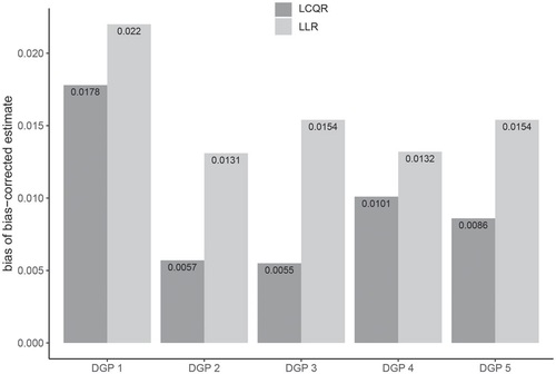
Table 3 Estimation of treatment effects in Lee and LM models.

Estimator	DGP 1		DGP 2		DGP 3		DGP 4		DGP 5
	coef.	s.e.	coef.	s.e.	coef.	s.e.	coef.	s.e.	coef.	s.e.
	A: Lee with homoscedastic errors and ${\tau }_{\text{sharp}}=0.04$
${\widehat{\tau }}_{1\text{bw}}^{\text{cqr}}$	0.071	0.188	0.061	0.228	0.062	0.250	0.061	0.204	0.058	0.250
${\widehat{\tau }}_{2\text{bw}}^{\text{cqr}}$	0.073	0.186	0.062	0.227	0.062	0.248	0.064	0.202	0.060	0.247
${\widehat{\tau }}_{1\text{bw}}^{\text{llr}}$	0.068	0.203	0.060	0.284	0.060	0.332	0.060	0.237	0.062	0.443
${\widehat{\tau }}_{1\text{bw}}^{\text{cqr},\text{bc}}$	0.058	0.347	0.046	0.411	0.046	0.454	0.050	0.375	0.049	0.453
${\widehat{\tau }}_{2\text{bw}}^{\text{cqr},\text{bc}}$	0.059	0.344	0.046	0.408	0.048	0.450	0.053	0.371	0.054	0.448
${\widehat{\tau }}_{1\text{bw}}^{\text{robust},\text{bc}}$	0.062	0.241	0.053	0.336	0.055	0.393	0.053	0.281	0.055	0.525
	B: Lee with heteroscedatic errors and ${\tau }_{\text{sharp}}=0.04$
${\widehat{\tau }}_{1\text{bw}}^{\text{cqr}}$	0.071	0.100	0.064	0.123	0.064	0.134	0.065	0.109	0.060	0.137
${\widehat{\tau }}_{2\text{bw}}^{\text{cqr}}$	0.072	0.099	0.064	0.122	0.063	0.133	0.066	0.108	0.062	0.133
${\widehat{\tau }}_{1\text{bw}}^{\text{llr}}$	0.067	0.116	0.062	0.163	0.061	0.190	0.062	0.136	0.063	0.255
${\widehat{\tau }}_{1\text{bw}}^{\text{cqr},\text{bc}}$	0.056	0.184	0.049	0.220	0.048	0.243	0.050	0.201	0.049	0.247
${\widehat{\tau }}_{2\text{bw}}^{\text{cqr},\text{bc}}$	0.057	0.183	0.048	0.219	0.049	0.242	0.051	0.199	0.050	0.241
${\widehat{\tau }}_{1\text{bw}}^{\text{robust},\text{bc}}$	0.061	0.138	0.055	0.193	0.056	0.226	0.056	0.161	0.057	0.303
	C: LM with homoscedasticity errors and ${\tau }_{\text{sharp}}=-3.45$
${\widehat{\tau }}_{1\text{bw}}^{\text{cqr}}$	−3.244	0.191	−3.265	0.231	−3.269	0.252	−3.257	0.206	−3.296	0.251
${\widehat{\tau }}_{2\text{bw}}^{\text{cqr}}$	−3.259	0.189	−3.280	0.228	−3.285	0.249	−3.270	0.204	−3.308	0.247
${\widehat{\tau }}_{1\text{bw}}^{\text{llr}}$	−3.340	0.223	−3.342	0.301	−3.333	0.346	−3.345	0.256	−3.328	0.452
${\widehat{\tau }}_{1\text{bw}}^{\text{cqr},\text{bc}}$	−3.439	0.353	−3.453	0.415	−3.450	0.458	−3.445	0.380	−3.443	0.455
${\widehat{\tau }}_{2\text{bw}}^{\text{cqr},\text{bc}}$	−3.440	0.348	−3.452	0.411	−3.450	0.452	−3.443	0.375	−3.440	0.447
${\widehat{\tau }}_{1\text{bw}}^{\text{robust},\text{bc}}$	−3.423	0.256	−3.434	0.349	−3.426	0.403	−3.432	0.295	−3.426	0.530
	D: LM with heteroscedatic errors and ${\tau }_{\text{sharp}}=-3.45$
${\widehat{\tau }}_{1\text{bw}}^{\text{cqr}}$	−3.234	0.106	−3.245	0.127	−3.252	0.138	−3.242	0.114	−3.281	0.137
${\widehat{\tau }}_{2\text{bw}}^{\text{cqr}}$	−3.239	0.104	−3.256	0.125	−3.259	0.136	−3.247	0.112	−3.288	0.134
${\widehat{\tau }}_{1\text{bw}}^{\text{llr}}$	−3.364	0.146	−3.359	0.190	−3.349	0.215	−3.364	0.165	−3.339	0.273
${\widehat{\tau }}_{1\text{bw}}^{\text{cqr},\text{bc}}$	−3.443	0.195	−3.448	0.228	−3.444	0.250	−3.442	0.209	−3.443	0.248
${\widehat{\tau }}_{2\text{bw}}^{\text{cqr},\text{bc}}$	−3.443	0.192	−3.447	0.225	−3.446	0.246	−3.444	0.206	−3.445	0.243
${\widehat{\tau }}_{1\text{bw}}^{\text{robust},\text{bc}}$	−3.431	0.163	−3.438	0.216	−3.432	0.245	−3.437	0.185	−3.431	0.315

NOTE: The estimates for the treatment effect and standard error are averages over 5000 replications with a sample size $n=500$. The s.e. and adjusted s.e. for LCQR are obtained using the asymptotic expressions from Theorem 1 and Theorem 3. Estimators with a superscript bc are both bias-corrected and s.e.-adjusted. The subscripts 1bw and 2bw refer to the use of equal and unequal bandwidths below and above the cutoff.

Table 3 further presents the standard errors of the studied estimators to facilitate comparison. The s.e. of ${\widehat{\tau }}_{1\text{bw}}^{\text{cqr}}$ is consistently smaller than that of ${\widehat{\tau }}_{1\text{bw}}^{\text{llr}}$, indicating the efficiency gain of LCQR against LLR. Although DGP 1 has normal errors, ${\widehat{\tau }}_{1\text{bw}}^{\text{cqr}}$ and ${\widehat{\tau }}_{1\text{bw}}^{\text{llr}}$ do not use the same bandwidth, so the s.e. of ${\widehat{\tau }}_{1\text{bw}}^{\text{cqr}}$ also appears smaller than that of ${\widehat{\tau }}_{1\text{bw}}^{\text{llr}}$. As the DGP moves away from normal errors, the LCQR estimator achieves various levels of efficiency gains compared to the LLR estimator. For example, the s.e. of ${\widehat{\tau }}_{1\text{bw}}^{\text{cqr}}$ in DGP 5 of Table 3 Panel B is 0.137, compared to 0.255 for ${\widehat{\tau }}_{1\text{bw}}^{\text{llr}}$, so the LCQR/LLR standard error ratio is close to 50% in this example.

While reading Table 3, it is important to bear in mind that the s.e.s of estimators with a superscript “bc” are not suitable to assess the efficiency of the estimators. They are computed by incorporating the additional variability due to bias correction. However, they shed light on the length of confidence intervals. Table 3 shows that the adjusted s.e. of ${\widehat{\tau }}_{1\text{bw}}^{\text{cqr},\text{bc}}$ could be smaller or larger than that of ${\widehat{\tau }}_{1\text{bw}}^{\text{robust},\text{bc}}$, so the simulation results for comparing LCQR with LLR appear to be mixed after bias correction.

In addition, using two bandwidths above and below the cutoff also gives mixed results in terms of bias correction for the LCQR estimator, though it is clear that the two-bandwidth approach leads to a small decrease in s.e. for LCQR.

5.2 Inference on the Treatment Effect

This subsection studies the coverage probability of the confidence intervals based on the LCQR estimator, using the adjusted s.e. in Theorem 3 and the adj. MSE-based bandwidth selector. The results are summarized in Table 4, where the nominal coverage probability is set to 95%.

Without bias correction or s.e. adjustment, confidence intervals based on the LCQR estimators, ${\widehat{\tau }}_{1\text{bw}}^{\text{cqr}}$ and ${\widehat{\tau }}_{2\text{bw}}^{\text{cqr}}$, are found to have poor coverage probabilities in Table 4, which highlights an important difference between estimation and inference: despite the excellent finite sample properties of LCQR in Table 3, one has to perform both bias correction and s.e. adjustment in order to produce the desired coverage of confidence intervals. Furthermore, the coverage probability of LCQR-based confidence intervals is lower than that of LLR-based confidence intervals. For example, it is 92.2% under DGP 1 in Panel A of Table 4, compared to 93.4% of the LLR-based confidence interval. Although ${\widehat{\tau }}_{1\text{bw}}^{\text{cqr}}$ tends to have a smaller bias and a smaller s.e. than ${\widehat{\tau }}_{1\text{bw}}^{\text{llr}}$, it appears that the bias in ${\widehat{\tau }}_{1\text{bw}}^{\text{cqr}}$ is still not small enough to center the estimator close to the true value. A smaller s.e. will further contribute to the decrease in coverage probabilities. This explains the poor coverage for confidence intervals based on ${\widehat{\tau }}_{1\text{bw}}^{\text{cqr}}$ and ${\widehat{\tau }}_{2\text{bw}}^{\text{cqr}}$.

With bias correction and s.e. adjustment, the proposed bandwidth selectors in Equations (39)(39) $$h_{Y_{+}}={\left(\frac{C_3}{6C_2^2}\right)}^{1/7}{n}_{+}^{-1/7},$$(39) and (40)(40) $$h={\left(\frac{C_{+,3}+C_{-,3}}{6{(C_{+,2}-C_{-,2})}^2}\right)}^{1/7}{n}^{-1/7}.$$(40) lead to good coverage across the five DGPs in Table 4. It is important to recall that the presented LCQR estimators use the bandwidths in Equations (39)(39) $$h_{Y_{+}}={\left(\frac{C_3}{6C_2^2}\right)}^{1/7}{n}_{+}^{-1/7},$$(39) and (40)(40) $$h={\left(\frac{C_{+,3}+C_{-,3}}{6{(C_{+,2}-C_{-,2})}^2}\right)}^{1/7}{n}^{-1/7}.$$(40) , which are not designed to optimize the coverage probability of confidence intervals, while the confidence intervals for ${\widehat{\tau }}_{1\text{bw}}^{\text{robust},\text{bc}}$ in Table 4 are optimized to minimize coverage errors. In this respect, it is reasonable to conclude that LCQR with bandwidths in Equations (39)(39) $$h_{Y_{+}}={\left(\frac{C_3}{6C_2^2}\right)}^{1/7}{n}_{+}^{-1/7},$$(39) and (40)(40) $$h={\left(\frac{C_{+,3}+C_{-,3}}{6{(C_{+,2}-C_{-,2})}^2}\right)}^{1/7}{n}^{-1/7}.$$(40) offers very competitive results.

In the last row of each panel in Table 4, we also report the coverage probability based on fixed-n approximations. The benefit of using fixed-n approximations becomes clearer in Table 6 of the online supplement, where the sample size decreases to 300 and fixed-n approximations often give the best coverage.

6 Application to Lee (2008)

In this section, we use the data from Lee (2008) to illustrate the practical usage of LCQR. To facilitate comparison, the findings based on LLR are also presented.

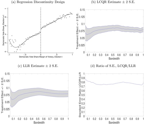
We revisit a classic example from Lee (2008) with 6558 observations depicted in Figure 2(a); see also Imbens and Kalyanaraman (2012). The horizontal running variable is the democratic vote share (margin of victory) in a previous election, while the vertical outcome variable is the democratic vote share in the election afterwards. Consistent with Lee (2008) and several follow-up studies, Figure 2(a) indicates that there is a positive impact of incumbency on re-election, that is, a visible jump occurs at the threshold zero.

Fig. 2 Comparison of LCQR and LLR using Lee (2008)

NOTES: (a) x-axis, the democratic vote share (margin of victory) in Election t; y-axis, the democratic vote share in Election t + 1. The dots show the sample mean of the vertical variable in each bin of the horizontal variable (50 bins on each side of the cutoff). The solid line represents the fitted fourth-order polynomial. As the bandwidth increases, (b) presents the LCQR estimate ± 2 × standard error; (c) presents the LLR estimate ± 2 × standard error; and (d) presents the ratio of the standard errors by LCQR and LLR. The MSE-optimal bandwidth of Imbens and Kalyanaraman (2012) for the studied dataset is about 0.3. The triangular kernel is used for both LCQR and LLR estimators.

Figure 2(b) and (c) presents the estimated impact of incumbency on re-election by LCQR and LLR methods, respectively. We consider a sequence of bandwidth values ranging from 0.05 to 1 with the step size 0.025: 0.05, 0.075, 0.1,…, 1. This bandwidth sequence thus nests many common choices such as the MSE-optimal bandwidth of Imbens and Kalyanaraman (2012), which is about 0.3 for the studied data.

The comparison of Figure 2(b) and (c) shows that LCQR and LLR yield similar point estimates over a wide range of bandwidths for the studied (Lee 2008) application. As the bandwidth increases, Figure 2(a) indicates that there are data points staying further away from the fitted regression line. These data points affect LCQR and LLR estimators in a different manner, leading to slightly disparate point estimates. Nevertheless, all the point estimates depicted in Figure 2(b) and (c) are significantly positive, since the (vertical) zero value is excluded from the shaded regions generated by ± 2 standard errors.

Most importantly, Figure 2(d) highlights that the standard error of the LCQR estimator is substantially smaller than that of LLR. The standard error ratio is mostly around 70%–80%, which can also be viewed by comparing the shaded regions in Figure 2(b) and (c). Moreover, this standard error ratio does not change much as the bandwidth varies. Thus, Figure 2(d) indicates that a confidence interval for the impact of incumbency on re-election based on the LCQR estimator could be considerably tighter than that by LLR.

Consider, for example, 0.3 as the adopted bandwidth. The LCQR estimate ± 1.96 standard error leads to the 95% confidence interval (0.068, 0.090), while the conventional 95% confidence interval by LLR is (0.065, 0.096). If bias correction is further accounted for at the adopted bandwidth 0.3, then the bias-corrected 95% confidence interval based on LCQR is (0.048, 0.090). This interval is comparable to the bias-corrected 95% confidence interval using the Calonico, Cattaneo, and Titiunik (2014) approach, which is (0.046, 0.089). These empirical findings therefore lend credibility to our proposed LCQR approach.

7 Conclusions

In this article, we study the application of LCQR in Kai, Li, and Zou (2010) to the estimation and inference in RD. We present numerical evidence for the efficiency gain of using LCQR in RD estimation, and also propose a bias-corrected and s.e.-adjusted t-statistic to improve the coverage of confidence intervals. Simulation results show good performance of the proposed method under several nonnormal error distributions.

The current work can be extended in several directions. For instance, throughout the article, we focus on the local linear composite quantile regression, while the general case, local pth-order polynomial composite quantile regression, can be similarly adopted. Kai, Li, and Zou (2009) establish the asymptotic theory for the LCQR estimator in the general case. Following Kai, Li, and Zou (2009), one could extend our results on the bias-corrected and s.e.-adjusted t-statistic to allow for higher-order polynomials. In addition, it will be naturally appealing to formally explore LCQR for kink RD designs as well as RD designs using covariates. It will also be interesting to revisit some of the existing applications in RD with the proposed method as data may deviate from normality. Finally, on the computation side, instead of using the same bandwidth for estimation, bias correction and s.e. adjustment, one can refine the bandwidth selection process, which may also improve the estimation and coverage probability of LCQR. We leave these topics for future research.

Acknowledgments

We thank the editor, the associate editor, and two anonymous referees for their comments that substantially improved the article.

Supplementary Materials

The related codes and data are provided in the R package rdcqr, which can be downloaded from the links in the article and the Supplement.

Additional information

Funding

The authors gratefully acknowledge the financial support of the Education Economics Center and the computational support of the Office of Research at Kennesaw State University, and have no conflicts of interest to disclose.

References

- Calonico, S., Cattaneo, M. D., and Farrell, M. H. (2018), “On the Effect of Bias Estimation on Coverage Accuracy in Nonparametric Inference,” Journal of the American Statistical Association, 113, 767–779. DOI: 10.1080/01621459.2017.1285776.
- Calonico, S., Cattaneo, M. D., and Farrell, M. H. (2020a), “Coverage Error Optimal Confidence Intervals for Local Polynomial Regression.” arXiv:1808.01398.
- Calonico, S., Cattaneo, M. D., and Farrell, M. H. (2020b), “Optimal Bandwidth Choice for Robust Bias-Corrected Inference in Regression Discontinuity Designs,” The Econometrics Journal, 23, 192–210.
- Calonico, S., Cattaneo, M. D., Farrell, M. H., and Titiunik, R. (2019), “Regression Discontinuity Designs Using Covariates,” The Review of Economics and Statistics, 101, 442–451. DOI: 10.1162/rest_a_00760.
- Calonico S., Cattaneo, M. D., and Titiunik, R. (2014), “Robust Nonparametric Confidence Intervals for Regression-Discontinuity Designs,” Econometrica, 82, 2295–2326. DOI: 10.3982/ECTA11757.
- Card, D., Lee, D. S., Pei, Z., and Weber, A. (2015), “Inference on Causal Effects in a Generalized Regression Kink Design,” Econometrica, 83, 2453–2483. DOI: 10.3982/ECTA11224.
- Cattaneo, M. D., Idrobo, N., and Titiunik, R. (2019), “A Practical Introduction to Regression Discontinuity Designs: Foundations,” Cambridge Elements: Quantitative and Computational Methods for Social Science, Cambridge: Cambridge University Press.
- Cattaneo, M. D., Idrobo, N., and Titiunik, R. (2020), “A Practical Introduction to Regression Discontinuity Designs: Extensions,” Cambridge Elements: Quantitative and Computational Methods for Social Science, Cambridge University Press.
- Fan, J., and Gijbels, I. (1996), Local Polynomial Modelling and Its Applications, London: CRC Press.
- Feir, D., Lemieux, T., and Marmer, V. (2016), “Weak Identification in Fuzzy Regression Discontinuity Designs,” Journal of Business and Economic Statistics, 34, 185–196. DOI: 10.1080/07350015.2015.1024836.
- Huang, X., and Lin, Z. (2021), “Local Composite Quantile Regression Smoothing: A Flexible Data Structure and Cross-Validation,” Econometric Theory, 37, 613–631. DOI: 10.1017/S0266466620000146.
- Imbens, G., and Kalyanaraman, K. (2012), “Optimal Bandwidth Choice for the Regression Discontinuity Estimator,” Review of Economic Studies, 79, 933–959. DOI: 10.1093/restud/rdr043.
- Imbens, G., and Lemieux, T. (2008), “Regression Discontinuity Designs: A Guide to Practice,” Journal of Econometrics, 142, 615–635. DOI: 10.1016/j.jeconom.2007.05.001.
- Kai, B., Li, R., and Zou, H. (2009), “Supplement Material for Local Composite Quantile Regression Smoothing: an Efficient and Safe Alternative to Local Polynomial Regression,” Technical Report. Pennsylvania State University, University Park.
- Kai, B., Li, R., and Zou, H. (2010), “Local Composite Quantile Regression Smoothing: An Efficient and Safe Alternative to Local Polynomial Regression,” Journal of the Royal Statistical Society, 72, 49–69.
- Kai, B., Li, R., and Zou, H. (2011), “New Efficient Estimation and Variable Selection Methods for Semiparametric Varying-Coefficient Partially Linear Models,” The Annals of Statistics, 39, 305.
- Lee, D. S. (2008), “Randomized Experiments From Non-Random Selection in us House Elections,” Journal of Econometrics, 142, 675–697. DOI: 10.1016/j.jeconom.2007.05.004.
- Li, D., and Li, R. (2016), “Local Composite Quantile Regression Smoothing for Harris Recurrent Markov Processes,” Journal of Econometrics, 194, 44–56. DOI: 10.1016/j.jeconom.2016.04.002.
- Ludwig, J., and Miller, D. L. (2007), “Does Head Start Improve Children’s Life Chances? Evidence From a Regression Discontinuity Design,” Quarterly Journal of Economics, 122, 159–208. DOI: 10.1162/qjec.122.1.159.
- Zhao, Z., and Xiao, Z. (2014), “Efficient Regressions Via Optimally Combining Quantile Information,” Econometric Theory, 30, 1272–1314. DOI: 10.1017/S0266466614000176.