Extreme Value Estimation for Heterogeneous Data

Abstract

We develop a universal econometric formulation of empirical power laws possibly driven by parameter heterogeneity. Our approach extends classical extreme value theory to specifying the tail behavior of the empirical distribution of a general dataset with possibly heterogeneous marginal distributions. We discuss several model examples that satisfy our conditions and demonstrate in simulations how heterogeneity may generate empirical power laws. We observe a cross-sectional power law for the U.S. stock losses and show that this tail behavior is largely driven by the heterogeneous volatilities of the individual assets.

Keywords:

• Extreme value theory
• Financial returns
• Heterogeneous data
• Power law
• Scales

1 Introduction

The empirical power law is a fundamental observation for many economic datasets: the tail probability seems to decrease at a polynomial rate rather than an exponential rate. It is also called the heavy-tailed phenomenon since large values occur more frequently than those from, for example, the (log)normal distribution in such a way that high-order sample moments may diverge with the sample size. At least since Pareto (1896) and Zipf (1949), the empirical power law has been well documented for income and wealth; see, for example, Piketty and Saez (2003) for the United States and France, Atkinson (2005) for the UK, the excellent book Piketty and Goldhammer (2014) for a general overview, and the recent survey Zucman (2019) for evidence across many countries. The heavy-tailed phenomenon extends enormously to various contexts, including city and firm size (e.g., Stanley et al. 1995; Gabaix 1999; Axtell 2001; Gabaix and Ioannides 2004; Schluter 2021), consumption (Toda and Walsh 2015), macroeconomic disasters (Barro and Jin 2011), social and economic networking (e.g., Barabási and Albert 1999; Jackson 2009; Newman, Barabási, and Watts 2006), CEO pay (Gabaix and Landier 2008), finance (e.g., Mandelbrot 1963; Fama 1963; Jansen and de Vries 1991; Longin 1996; Gopikrishnan et al. 1999; Gopikrishnan et al. 2000; Gabaix et al. 2006; Plerou and Stanley 2007; Kyle and Obizhaeva 2016), international trade (di Giovanni, Levchenko, and Rancière 2011; di Giovanni and Levchenko 2012), and many others. For more examples in economics and finance we refer to the excellent surveys Gabaix (2009) and Gabaix (2016). For many examples beyond economics, we refer to, for example, the survey Clauset, Shalizi, and Newman (2009).

The larger observations are often depicted in a log–log plot: plot on logarithmic axes the data ranks in the descending order as a function of the data values. In Figure 1, we observe a linear pattern in these plots that identifies empirical power laws for four data examples:

Fig. 1 Empirical power laws in log–log plots. The axes are logarithmic.

1. Census 2010 resident population in millions for the largest 100 U.S. cities collected from the online database of the U.S. Census Bureau, Population Division.

2. The largest 50 numbers of citations, as of June 1997, of the articles cited at least once which were published in volumes 11 through 50 of Physical Review D (Redner 1998).

3. The largest 50 monthly stock returns in March 2020 on the largest 1000 U.S. companies with share codes 10 and 11 collected from the Center for Research in Security Prices (CRSP).

4. The wealth of top 100 billionaires among the Forbes richest 400 Americans in 2019.

Denote an entire dataset by $(X_1^{(p)},\dots ,X_p^{(p)})$ where the data dimension p is large, and define its empirical distribution function (df) by(1.1) $$F_{\text{emp}}(x)=\frac{1}{p}\sum _{i=1}^{p}1(X_i^{(p)}\le x).$$(1.1)

The fitted straight line in each log–log plot supports the empirical power law, that is,(1.2) $$1-F_{\text{emp}}(x)\mathrm{ }\text{is}\mathrm{ }\text{approximately}\mathrm{ }{x}^{-1/\widehat{\gamma }}\mathrm{ }\text{for}\mathrm{ }\text{large}\mathrm{ }x,$$(1.2) where $-1/\widehat{\gamma }$ is the slope of the fitted line and $\widehat{\gamma }$ is the estimated Extreme Value Index (EVI). The larger the estimated EVI $\widehat{\gamma }$, the heavier the tail.

In contrast to the increasing complexity of the economic generating mechanisms, the explanation of the power law is remarkably straightforward from a probabilistic point of view. The seminal works by Fisher and Tippett (1928) and Gnedenko (1943) showed that the asymptotic distribution of the maximum of a random sample, up to proper standardization, can only take a specific form depending on a single parameter γ, called the EVI. An equivalent formulation of these results by Balkema and de Haan (1974) and Pickands (1975) showed that the conditional excess distribution beyond a sufficiently large threshold can only approach a generalized Pareto law. The power law immediately follows from the limiting generalized Pareto distribution in case the EVI γ is positive. Historically, these two formulations of the power law led to two different statistical characterizations of empirical power laws, the so-called block-maxima method and peaks-over-threshold method, that model the maxima over subsamples and all large observations in the full sample, respectively. Our log–log plot in Figure 1 uses the latter one. For excellent accounts of extreme value theory, we refer to the books Embrechts, Klüppelberg, and Mikosch (1997), de Haan and Ferreira (2006), and Resnick (2007). For similar results under weak temporal dependence; see, for example, Leadbetter, Lindgren, and Rootzén (1983). Extreme value theory for data generated from a mixture process has recently been developed in Cao and Zhang (2020).

A caveat of the aforementioned classical extreme value theory is that it works with homogeneous, that is, equally distributed data. In fact, Hüsler (1986) showed that the standard formulation does not generalize to arbitrary nonstationary data. This immediately raises questions to econometricians who are dealing with power laws of heterogeneous economic data at a given point in time or dynamic cross-sectional data over time; see, for example, Allen, Bali, and Tang (2012), Kelly and Jiang (2014), and Gabaix et al. (2016). For all practical purposes, however, economists tend to disregard the statistical complexity by directly working with data from a common distribution. This convenience comes at an obvious cost of neglecting the micro heterogeneity, which is then absorbed in the common hypothetical macro distribution. One possible endorsement for such an approach was given recently in Einmahl, de Haan, and Zhou (2016), which shows that the estimated EVI $\widehat{\gamma }$ is still consistent for the common EVI γ for heavy-tailed data if they only differ by scale in the tail. In contrast, as we show later on, in general the heterogeneity effect is not only nonnegligible, but also can generate a positive γ, that is, a heavy tail, even for light-tailed Gaussian data.

The motivation of this article is to formalize the econometric theory for the aforementioned practical approach adopted by economists. In Section 2, we introduce Chang’s condition, see Chang (1955) and also Wellner (1978), that states that in the intermediate tail the empirical df $F_{\text{emp}}$ of possibly heterogeneous data approaches some limiting df F. Note that Chang’s condition requires no specific form of the dependence structure nor tail homogeneity of the data. We then show that the estimated EVI converges to the EVI of the limiting distribution under a weak stability condition. Most importantly, now we can interpret the empirical power law as a finite sample approximation if the limiting distribution is heavy-tailed.

To illustrate how the micro heterogeneity influences the limiting df, we derive this limiting df and verify Chang’s condition for various interesting models in Section 3. These models reveal that, as noted above, the heavy tail may be directly generated by the parameter heterogeneity of the dataset even if each individual observation comes from a light-tailed distribution.

We then demonstrate how heterogeneity may generate the dynamics of empirical power laws by simulations in Section 4. Our data generating processes are calibrations based on the U.S. income inequality data and financial data. Our model can replicate the rapid rise in the U.S. income inequality, which is driven by the scale heterogeneity of the cross-sectional data. Heterogeneity is a fundamental property of individual incomes (see, e.g., Fagereng et al. 2020), and our analysis may provide new insights into the dynamics of inequality (Gabaix et al. 2016). Furthermore, our model also suggests that pooling heterogeneous EGARCH data over time may significantly reduce the variability of the EVI estimator but not so much the estimation bias (Kelly and Jiang 2014).

Finally, in Section 5, we study cross-sectional daily U.S. stock losses and observe a persistent power law behavior for the entire 10-year period as well as for the 120 periods of a single month. We show that this tail behavior is largely driven by the heterogeneous volatilities of the individual assets.

The proofs of the results in Sections 2 and 3 are deferred to appendix.

2 Unified Estimation Theory for Empirical Power Laws

Throughout we denote our data vector by $X=(X_1^{(p)},\dots ,X_p^{(p)})$, where the dimension p is large. In general, X is an arbitrary high-dimensional random vector with unspecified dependence structure and possibly heterogeneous tail distributions. Typically, these data are cross-sectional observations given at a point in time or a pool of possibly imbalanced panel data over a certain time period. Let the empirical df be as defined in (1.1)(1.1) $$F_{\text{emp}}(x)=\frac{1}{p}\sum _{i=1}^{p}1(X_i^{(p)}\le x).$$(1.1) . For any probability df F on $\mathbb{R}$, we define its generalized quantile function by $Q(t)=\inf \{x\in \mathbb{R}:F(x)\ge t\}$.

Our theory relies on the following assumption, which is established in Chang (1955) for iid data.

Assumption 1

(Chang’s condition). In the intermediate tail, the empirical df $F_{\text{emp}}$ approaches some increasing df F in such a way that$$\underset{c\le x\le Q(1-a)}{\sup }\left|\frac{1-F_{\text{emp}}(x)}{1-F(x)}-1\right|\stackrel{\mathbb{P}}{\to }0,\hspace{1em}p\to \infty ,$$for some c > 0 and all sequences $a=a(p)\to 0$ such that $pa\to \infty ,a\in (0,1)$.

The universe of limiting dfs F is diversified and F may or may not have a heavy tail. Note that the assumption allows even a deterministic data vector X, such as the growth rate parameters of individuals, stock volatilities or market betas in a cross section. The lower bound c being nondivergent ensures that the limiting df F is unique at each fixed point $x\ge c$. To relax this condition, if necessary, one may replace c by another intermediate quantile sequence as in Gardes (2015) and our asymptotic theory generalizes.

For tail inference, we further assume that the limiting distribution is heavy-tailed.

Assumption 2

(Regular variation). The df F is heavy-tailed, that is, is in the maximum domain of attraction with EVI $\gamma >0$. In other words, the survival function $1-F$ is regularly varying at infinity with index $-\frac{1}{\gamma }$:$$\underset{t\to \infty }{\lim }\frac{1-F(tx)}{1-F(t)}=x^{-1/\gamma },\hspace{1em}x>0.$$

The EVI quantifies the tail heaviness of F: the larger γ, the heavier tail and less finite moments F has.

Combining Assumptions 1 and 2, one may now interpret the empirical power laws (1.2)(1.2) $$1-F_{\text{emp}}(x)\mathrm{ }\text{is}\mathrm{ }\text{approximately}\mathrm{ }{x}^{-1/\widehat{\gamma }}\mathrm{ }\text{for}\mathrm{ }\text{large}\mathrm{ }x,$$(1.2) from an asymptotic perspective: the empirical power law is a finite sample approximation of that of the limiting df F. Our model suggests that, if the practitioners believe that the data exhibit certain tail behavior, the power law is the only possible observation under regular variation. This may explain why the power law is such a widely observed phenomenon in real-life datasets.

As noted in the Introduction, our interest is to estimate the tail of the limiting df F which reflects the asymptotic behavior of the larger observations. The rationale is similar to that behind fitting lines in the empirical power law plots as in the Introduction. Specifically, we order the data to obtain the largest k + 1 order statistics given by $X_{p-k:p}\le X_{p-k+1:p}\le \cdots \le X_{p-1:p}\le X_{p:p}$ for estimation, where $k=k(p)\in \{1,\dots ,p-1\}$ is such that

Assumption 3.

$k/\hspace{0.17em}\text{log}\hspace{0.17em}p\to \infty$ and $k/p\to 0$ as $p\to \infty$.

Note that in our very general setting, the usual condition that $k\to \infty$ has to be strengthened slightly. Often k is taken proportional to $p^{\beta }$, for some $\beta \in (0,1)$, and then, of course, $k/\hspace{0.17em}\text{log}\hspace{0.17em}p\to \infty$ is amply satisfied.

We use the Hill (1975) estimator of the EVI $\gamma >0$ given by(2.1) $$\widehat{\gamma }=\frac{1}{k}\sum _{i=0}^{k-1}\hspace{0.17em}\text{log}\hspace{0.17em}{X}_{p-i:p}-\hspace{0.17em}\text{log}\hspace{0.17em}{X}_{p-k:p},$$(2.1) which is the sample average of the excesses over the intermediate quantile $X_{p-k:p}$, on a log scale.

To exclude the very irregular cases where the sample maximum dominates the estimator, we require

Assumption 4

(Stability condition). $\text{log}\hspace{0.17em}{X}_{p:p}=O_{\mathbb{P}}(\hspace{0.17em}\text{log}\hspace{0.17em}p)$, as $p\to \infty$.

If the data are iid observations from F, then this condition is readily satisfied under the regular variation Assumption 2 for any positive γ (see, e.g., de Haan and Ferreira 2006, chap. 1). We argue that this condition is very mild in practice, as the largest point often does not overwhelm the fitting process in the log–log plots such as those in the Introduction.

Now, our unified consistency theorem for empirical power laws is as follows:

Theorem 1.

Under Assumptions 1–4, we have, as $p\to \infty$,$$\widehat{\gamma }\stackrel{\mathbb{P}}{\to }\gamma .$$

3 Applications to Heterogeneous Econometric Models

In this section, we present and discuss some interesting examples of heterogeneous data that satisfy our assumptions and hence the Hill estimator is consistent in those settings.

Our first example is a generalization of the heteroscedastic extremes model in Einmahl, de Haan, and Zhou (2016). Let $X=(X_1^{(p)},\dots ,X_p^{(p)})$ have independent entries with continuous dfs $F_{p,1},\dots ,F_{p,p}$. Suppose there exists a df F and a set of nonnegative constants $\left\{c_{p,i}\right\}$ such that$$\underset{x\to \infty }{\lim }\frac{1-F_{p,i}(x)}{1-F(x)}=c_{p,i}$$uniformly for all p and $1\le i\le p$, where $\frac{1}{p}{\sum }_{i=1}^p{c}_{p,i}\to 1$, as $p\to \infty$. Furthermore, assume that the $\left\{c_{p,i}\right\}$ are bounded and that the $\{c_{p,i}:c_{p,i}>0\}$ are bounded away from zero.

Theorem 2

(Heteroscedastic extremes). For this generalized heteroscedastic extremes model, Chang’s condition (Assumption 1) holds. Furthermore, if F satisfies the regular variation condition (Assumption 2), then the stability condition (Assumption 4) holds.

Our second example is a heterogeneous scales model defined by$$X_i^{(p)}=\mu +{\sigma }_{p,i}{Z}_i,\hspace{1em}i=1,2,\dots ,p,\hspace{1em}\mu \in \mathbb{R},$$where the Z_i are iid random variables with df G and the ${\sigma }_{p,1}\le {\sigma }_{p,2}\le \cdots \le {\sigma }_{p,p}$ are positive scale parameters. We assume that the scale parameters resemble the intermediate quantiles of a continuous df $F_{\sigma }$, with positive left endpoint, in such a way that ${\sigma }_{p,i}/Q_{\sigma }(i/p)\to 1$ uniformly for $1\le i\le (1-a)p$, for all intermediate sequences $a=a(p)\to 0$ such that $pa\to \infty$. We require that $Q_{\sigma }$ is continuous on $(0,1]$ and that for some $t^{+}\in (0,1)$,(3.1) $$\underset{\delta \downarrow 0}{\lim }\underset{0<t\le t^{+},|s/t-1|\le \delta }{\sup }|Q_{\sigma }(1-s)/Q_{\sigma }(1-t)-1|=0.$$(3.1)

Theorem 3

(Heterogeneous scales). For the heterogeneous scales model, if F defined by $F(x)={\int }_0^{\infty }G\left(\frac{x-\mu }{s}\right)d{F}_{\sigma }(s),x\in \mathbb{R}$, satisfies Assumption 2, then Chang’s condition (Assumption 1) holds. Furthermore, if, for some $\alpha >0,1-G(x)\le x^{-\alpha }$, for large x, and ${\sigma }_{p,p}\le p^{1/\alpha }$, for large p, then the stability condition holds.

It easily follows that if Y has df $F_{\sigma }$ and is independent of Z₁, then $\mu +Y{Z}_1$ has df F as in this theorem. If $F_{\sigma }$ satisfies Assumption 2, and G has a not-heavier tail, that is, $\underset{x\to \infty }{\lim }\frac{1-G(x)}{1-F_{\sigma }(x)}\in [0,\infty )$, then the limiting F has the same EVI as $F_{\sigma }$, see Lemma 4.1 in the survey article Jessen and Mikosch (2006). When G has a heavier tail than $F_{\sigma }$, that is, $\underset{x\to \infty }{\lim }\frac{1-G(x)}{1-F_{\sigma }(x)}=\infty$, and G satisfies Assumption 2, F has the same EVI as G. In other words, either the scale parameter heterogeneity or the tail of the marginal variables may generate a heavy tail.

Corollary 1

(High-dimensional Gaussian vector with heterogeneous scales). Suppose that the heterogeneous scales model holds with$$X_i^{(p)}\sim \mathcal{N}\left(\mu ,{\sigma }_{p,i}^2\right), i=1,\dots ,p,$$where $F_{\sigma }$ satisfies Assumption 2 with $\gamma >0$. Then Chang’s condition holds with F as in the theorem and G the standard normal df; F is heavy-tailed with the same γ as $F_{\sigma }$.

In this situation, the empirical power law is driven by the heterogeneity of the scales instead of the tail behavior of the marginal variables.

The next corollary to Theorem 3 generalizes it to a certain type of dependent data.

Corollary 2

(Heterogeneous scales and dependence). Consider the heterogeneous scales setup in and above Theorem 3, with μ = 0. Let Y > 0 be a random variable and define$${\tilde{X}}_i^{(p)}=Y{X}_i^{(p)},\hspace{1em}i=1,\dots ,p.$$

Let $\tilde{\gamma }$ be the Hill estimator of the ${\tilde{X}}_i^{(p)}$ and $\widehat{\gamma }$ the Hill estimator of the $X_i^{(p)}$. Then $\tilde{\gamma }=\widehat{\gamma }$ and hence $\tilde{\gamma }\stackrel{\mathbb{P}}{\to }\gamma .$

Remark 1

(High-dimensional lognormal vector with dependent components and heterogeneous scales). An interesting example of the ${\tilde{X}}_i^{(p)}$ is obtained by taking $Y=\hspace{0.17em}\text{exp}\hspace{0.17em}(Z)$, with $Z\sim N(0,\rho {\sigma }^2),{\sigma }^2>0,0<\rho \le 1$, and $X_i^{(p)}={\sigma }_{p,i}\hspace{0.17em}\text{exp}\hspace{0.17em}({\tilde{Z}}_i)$ with ${\tilde{Z}}_i,i=1,\dots ,p$, independent and $N(0,(1-\rho ){\sigma }^2)$-distributed. In this case ${\tilde{X}}_i^{(p)}={\sigma }_{p,i}\hspace{0.17em}\text{exp}\hspace{0.17em}(Z+{\tilde{Z}}_i)$ and $(Z+{\tilde{Z}}_1,\dots ,Z+{\tilde{Z}}_p)$ is multivariate normal with all correlations equal to ρ. Clearly, the ${\tilde{X}}_i^{(p)}$ are dependent and all have a lognormal distribution.

The next example is a heterogeneous locations model defined by$$X_i^{(p)}={\mu }_{p,i}+Z_i,\hspace{1em}i=1,2,\dots ,p,$$where the Z_i are iid random variables with df G and the ${\mu }_{p,1}\le \cdots \le {\mu }_{p,p}$ are location parameters. Suppose that for some continuous df $F_{\mu }$ and some weight function $q:(0,1)\to (0,\infty )$ it holds that(3.2) $${\max }_{ap\le i\le (1-a)p}\frac{\left|{\mu }_{p,i}-Q_{\mu }(i/p)\right|}{q(i/p)}\to 0,$$(3.2) for all sequences $a=a(p)\to 0$ such that $pa\to \infty$. Define for $\eta \in \mathbb{R}$,$$F_{(\eta )}(x)={\int }_0^{1}G\left(x-Q_{\mu }(t)-\eta q(t)\right)dt,x\in \mathbb{R},$$ and write F for $F_{(0)}$.

Theorem 4

(Heterogeneous locations). Assume

1. $\underset{\eta \to 0}{\lim }\underset{x\ge c}{\sup }\left|\frac{1-F_{(\eta )}(x)}{1-F(x)}-1\right|=0$ for some c,

2. $\underset{\delta \downarrow 0}{\lim }\underset{0<t\le 1/2,|s/t-1|\le \delta }{\sup }\left\{\mathrm{}\mathrm{}\frac{\left|\mathrm{}{Q}_{\mu }(s)-Q_{\mu }(t)\mathrm{}\right|}{q(t)}+\frac{\left|\mathrm{}{Q}_{\mu }(1-s)-Q_{\mu }(1-t)\mathrm{}\right|}{q(1-t)}\mathrm{}\mathrm{}\right\}=0$,

3. $\underset{\delta \downarrow 0}{\lim }\underset{0<t\le 1/2,|s/t-1|\le \delta }{\sup }\left\{\left|\frac{q(s)}{q(t)}-1\right|+\left|\frac{q(1-s)}{q(1-t)}-1\right|\right\}=0.$

Then Chang’s condition holds. Furthermore, if, for some $\alpha >0,1-G(x)\le x^{-\alpha }$ and ${\mu }_{p,p}\le p^{1/\alpha }$ for large p, then the stability condition holds.

It readily follows that if Y has df $F_{\mu }$ and is independent of Z₁, then $Y+Z_1$ has df $F=F_{(0)}$ as defined above the theorem. The limiting df F has the same EVI γ as that of $F_{\mu }$, if $F_{\mu }$ satisfies Assumption 2, when G has a not-heavier tail such that $\underset{x\to \infty }{\lim }\frac{1-G(x)}{1-F_{\mu }(x)}\in [0,\infty )$ by the proposition on (Feller 1978, p. 278) about convolutions of regular varying distributions; see also Lemma 3.1 in Jessen and Mikosch (2006). When G has a heavier tail than $F_{\mu }$, that is, $\underset{x\to \infty }{\lim }\frac{1-G(x)}{1-F_{\mu }(x)}=\infty$, the limiting df F has the same EVI as G if G satisfies Assumption 2 with a positive EVI γ. In other words, both the location parameter heterogeneity or the tail of the marginal variables may generate a heavy tail.

The examples in Theorems 2–4 and many other examples can be generalized to the setup where many small possibly heterogeneous sets of possibly dependent observations are pooled. This situation can also be seen as a (general, unbalanced) panel data setup. Let T be a fixed, positive integer. Consider data $X_{i,t}$, with $i=1,\dots ,p^{*}$, and $$, where ${\mathcal{T}}_i$ is a nonempty subset of $\{1,\dots ,T\}$, for all $1\le i\le p^{*}$. Now, for the asymptotic theory, we assume that for each fixed $t\in \{1,\dots ,T\}$, the number of data points $X_{i,t}$ either tends to infinity or stays bounded, as $p^{*}\to \infty$. Let p_t be the number of $X_{i,t}$ and denote with ${\mathcal{T}}_{\infty }$ those t for which $p_t\to \infty$ as $p^{*}\to \infty$; naturally we require ${\mathcal{T}}_{\infty }\ne \varnothing$. Note that the data $X_{i,t}$ may be dependent here.

Theorem 5.

Assume that for each fixed $t\in {\mathcal{T}}_{\infty }$, the data $X_{i,t}$ satisfy Chang’s condition with F = F_t and p = p_t . Let $p={\sum }_{t=1}^T{p}_t$ and assume, for $t\in {\mathcal{T}}_{\infty }$, that $\underset{p^{*}\to \infty }{\lim }{p}_t/p=w_t>0$. Consider the empirical df $F_{\text{emp}}$ of all p random variables $X_{i,t}$. Define $F=\sum _{t\in {\mathcal{T}}_{\infty }}{w}_t{F}_t$ and assume F is continuous. Then, as $p\to \infty$, Chang’s condition holds. Denote with $H_{i,t}$ the df of $X_{i,t}$ and assume for all i and t with $t\notin {\mathcal{T}}_{\infty }$ that for large x, $H_{i,t}(x)\ge H(x)$ for some fixed df H. Then, if for each fixed $t\in {\mathcal{T}}_{\infty }$, the stability condition holds with p = p_t , then the stability condition holds for the maximum $X_{p:p}$ of all p data.

This theorem states that, quite generally, Chang’s condition and the stability condition remain valid under pooling. Nothing is required for the data subset $\left\{X_{i,t}\right\}$, for fixed i. As proved in Section 2, these two conditions lead to the consistency of the Hill estimator if k is chosen according to Assumption 3 and if F satisfies Assumption 2. The latter assumption follows easily, if the individual $F_t,t\in {\mathcal{T}}_{\infty }$, satisfy it for some ${\gamma }_t>0$ (but this can be weakened). The pooled or panel data setup provides a very general setting where consistency of the Hill estimator is established.

4 Simulation Study

In this section, we present a simulation study to demonstrate how heterogeneous data generate heavy tails in high dimensions and to evaluate the finite sample performance of the Hill estimator. We consider three data-generating processes:

1. Heterogeneous lognormal variables $X_i^{(p)}={\sigma }_{p,i}\hspace{0.17em}\text{exp}\hspace{0.17em}(Z_i)$ with $(Z_1,\dots ,Z_p)$ centered multivariate normal with all variances equal to $\sigma =0.3$ and a common correlation $\rho \in [0,1]$. The scale parameters ${\sigma }_{p,i}$ are the quantiles at probability level $\frac{i+p-1}{2p}$ of the log-logistic distribution (Fisk 1961) with unit median and $\gamma =0.39$.

2. Heterogeneous lognormal variables $\{X_{i,t}^{(p)}:i=1,\dots ,p\}$ at fixed time t generated from the autoregressive model$$\text{log}\hspace{0.17em}{X}_{i,s}^{(p)}=\lambda \hspace{0.17em}\text{log}\hspace{0.17em}{\sigma }_{p,i}+\varphi \hspace{0.17em}\text{log}\hspace{0.17em}{X}_{i,s-1}^{(p)}+{\epsilon }_{i,s}, s=1,\dots ,t,$$

with $\lambda =0.1,\varphi =0.94$ and initial values $X_{i,0}^{(p)}={\sigma }_{p,i}\hspace{0.17em}\text{exp}\hspace{0.17em}(Z_i)$ generated from DGP I with independent $Z_i\sim N(0,{\sigma }^2)$ with $\sigma =0.3$. We generate the iid errors ${\epsilon }_{i,s}\sim N(0,{\sigma }_{\epsilon }^2)$, independent of the initial values $\left\{X_{i,0}^{(p)}\right\}$, with ${\sigma }_{\epsilon }=\frac{\lambda \sqrt{1-{\varphi }^2}}{1-\varphi }\sigma =0.17$.

1. A pooled dataset of heterogeneous EGARCH(1,1) data $\{X_{i,t}^{(p)}:i=1,\dots ,p,t=1,\dots ,T\}$ such that$$\{\begin{array}{c}{X}_{i,t}^{(p)}=\sqrt{h_{i,t}^{(p)}}{Z}_{i,t}\hfill \\ \hspace{0.17em}\text{log}\hspace{0.17em}{h}_{i,t}^{(p)}=0.2\hspace{0.17em}\text{log}\hspace{0.17em}{\sigma }_{p,i}^2+0.1Z_{i,t-1}+0.8\hspace{0.17em}\text{log}\hspace{0.17em}{h}_{i,t-1}^{(p)}\hfill \end{array}$$

where the $Z_{i,t}\sim N(0,1)$ are independent errors and the scale parameters $\left\{{\sigma }_{p,i}\right\}$ are the same as in DGP I. We use the initial values $h_{i,1}^{(p)}={\sigma }_{p,i}^2$.

All three DGPs satisfy the (pooled) heterogeneous scales model in Section 3. The extreme value indices (EVIs) of DGP I and II are calibrated by using the empirical EVIs for United States income distributions from 1973 to 2018, as shown in Figure 2. The empirical EVIs (blue line) are calculated as $1+{\hspace{0.17em}\text{log}\hspace{0.17em}}_{10}\frac{S(0.1)}{S(1)}$, where S(p) denotes the share of the top pth percentile of the income data taken from Piketty and Saez (2003, tab. A.1) and the updated dataset downloaded at: https://eml.berkeley.edu/ saez/TabFig2018.xls. For DGP I and the initial values in DGP II, we have set the cross-sectional EVI $\gamma =0.39$ equal to the empirical EVI of 1973. For DGP II, the cross-sectional EVIs change over time and obey the first-order difference equation$${\gamma }_t=0.1\gamma +0.94{\gamma }_{t-1}=0.039+0.94{\gamma }_{t-1},$$where γ_t denotes the cross-sectional EVI at time t (or year $1973+t$ in Figure 2), and the intercept 0.039 and the autoregressive coefficient 0.94 are the least-square estimates for the time series of empirical EVIs. Our model can replicate the rapid rise in the U.S. income inequality and implies a long-run steady state $\underset{t\to \infty }{\lim }{\gamma }_t=0.65$. For each time period t, the cross-sectional dataset in DGP II can be rewritten as a heterogeneous scales model$$X_{i,t}^{(p)}={\left({\sigma }_{p,i}\hspace{0.17em}\text{exp}\hspace{0.17em}\left({\tilde{Z}}_{i,t}\right)\right)}^{{\gamma }_t/\gamma }={\sigma }_{p,i}^{{\gamma }_t/\gamma }\hspace{0.17em}\text{exp}\hspace{0.17em}\left(Z_{i,t}\right),$$$${\tilde{Z}}_{i,t}=\frac{{\gamma }_t}{\gamma }{Z}_{i,t}\sim N\left(0,{\sigma }_t^2\right),$$ where$${\sigma }_t^2=(1-{\rho }_t){\sigma }^2, {\rho }_t=1-{\left(\frac{\gamma }{{\gamma }_t}\right)}^2\left({\varphi }^{2t}+\frac{1-{\varphi }^{2t}}{1-{\varphi }^2}\frac{{\sigma }_{\epsilon }^2}{{\sigma }^2}\right).$$

Fig. 2 Empirical extreme value indices and calibrated extreme value indices for U.S. income (excluding capital gains) distributions between 1973 and 2018.

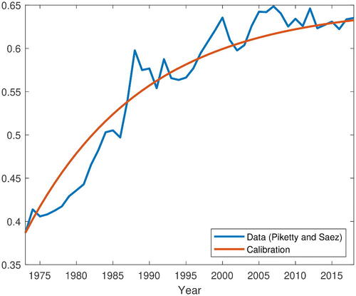
Table 1 Average and mean absolute deviation of the relative estimation errors $\widehat{\gamma }/\gamma -1$ based on 5000 replications for dimension p = 200, 1000, and 5000.

DGP I: $$
p	$\rho =0.00$	$\rho =0.25$	$\rho =0.50$	$\rho =0.75$	$\rho =1.00$
200	–0.031 (0.117)	–0.036 (0.110)	–0.040 (0.101)	–0.044 (0.084)	–0.045 (0.000)
1000	–0.017 (0.075)	–0.020 (0.069)	–0.021 (0.062)	–0.022 (0.053)	–0.025 (0.000)
5000	–0.008 (0.046)	–0.011 (0.043)	–0.011 (0.039)	–0.012 (0.033)	–0.012 (0.000)
DGP II: ${\gamma }_t=0.039+0.94{\gamma }_{t-1},{\gamma }_0=0.39$
p	t = 1	t = 26	t = 51	t = 75	t = 100
200	–0.004 (0.095)	–0.018 (0.124)	–0.026 (0.120)	–0.024 (0.120)	–0.027 (0.119)
1000	0.016 (0.061)	–0.008 (0.076)	–0.015 (0.074)	–0.017 (0.074)	–0.017 (0.074)
5000	0.028 (0.037)	–0.001 (0.048)	–0.006 (0.047)	–0.008 (0.046)	–0.008 (0.046)
DGP III: $\gamma =0.39$
p	T = 1	T = 2	T = 3	T = 4	T = 5
200	–0.008 (0.132)	–0.011 (0.096)	–0.013 (0.077)	–0.016 (0.068)	–0.015 (0.062)
1000	–0.006 (0.086)	–0.005 (0.060)	–0.009 (0.050)	–0.010 (0.042)	–0.010 (0.038)
5000	–0.004 (0.054)	–0.004 (0.038)	–0.005 (0.031)	–0.004 (0.027)	–0.005 (0.024)

Although the cross-sectional data are independent at time t, the distribution of the Hill estimator is equivalent to that for a power transformation of DGP I with correlation $\rho ={\rho }_t$ after cancelling the common random scale component; see Remark 1. We have chosen ${\sigma }_{\epsilon }=\frac{\lambda \sqrt{1-{\varphi }^2}}{1-\varphi }\sigma$ such that ρ_t dies out in the long run, that is,$$\underset{t\to \infty }{\lim }{\rho }_t=1-{\left(\frac{1-\varphi }{\lambda }\right)}^2·\frac{1}{1-{\varphi }^2}\frac{{\sigma }_{\epsilon }^2}{{\sigma }^2}=0.$$

We argue that ${\sigma }_{\epsilon }=0.17$ is a reasonably calibrated volatility for (high) income growth; see, e.g., Gabaix et al. (2016). Finally, DGP III is motivated by the financial applications in Kelly and Jiang (2014), where all the daily (idiosyncratic) stock losses in the same month are pooled for the monthly estimation. We have chosen the initial values of $h_{i,t}$ such that the cross-sectional EVIs stabilize over time t for simplicity; otherwise, the cross-sectional EVIs follow a similar dynamics as DGP II.

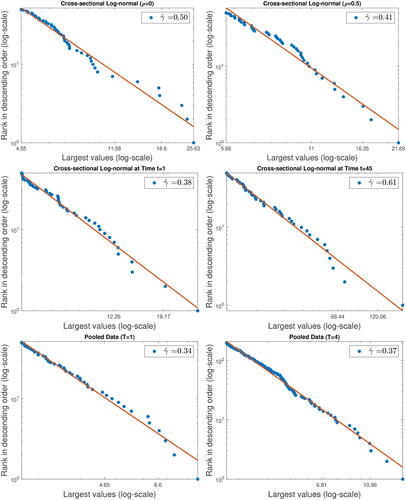
Figure 3 shows the log-log plots for the largest 5% values from one sample of size p = 1000 from DGP I–III. From the first row, for DGP I, we observe that the Hill estimate is closer to the true value $\gamma =0.39$ for the larger ρ. In the second row, for DGP II, we report the estimates for t = 1 (year 1974) and t = 45 (year 2018). The Hill estimates are both close to the true empirical EVIs, which are different over time as discussed above. In the last row, for DGP III, we observe that the Hill estimate for the pooled data with T = 4 is slightly closer to the true value than that for T = 1.

Fig. 3 Empirical power laws in log-log plots for one sample with p = 1000.

To demonstrate the convergence of the Hill estimator as the dimension p grows, we report in Table 1, the average and mean absolute deviation of the relative estimation error of the Hill estimates against the true values based on 5000 replications for dimension p = 200, 1000, and 5000 with k is equal to 10%, 5%, and 2.5% of the dimension p for DGP I and II and of the pooled sample size pT for DGP III, respectively. In general, the absolute bias and the variability decrease as the dimension p grows for all DGPs, in line with the consistency of the Hill estimator. For DGP I, the mean absolute deviation decreases as the correlation ρ grows. This is because the Hill estimator is invariant with respect to the factor Y in Remark 1, while the idiosyncratic component ${\tilde{Z}}_i$ there has a decreasing variance as ρ grows. Indeed, in the extreme case with ρ = 1, the Hill estimator is fully driven by the parameters and becomes deterministic. For DGP II, for each p, the bias and variability of the Hill estimator stabilize as t grows and approaches that for DGP I with ρ = 0 by construction. For DGP III, pooling the cross-sectional data over multiple time periods yields a larger sample size and hence smaller variability.

5 Empirical Analysis of the U.S. Stock Data

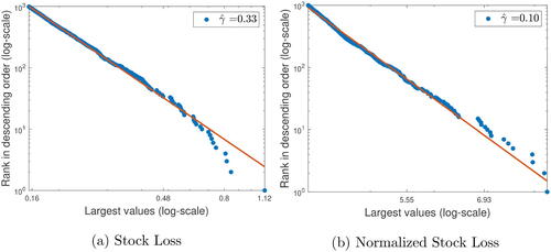
In this section, we study the cross-sectional empirical power laws of the U.S. asset returns. Our dataset contains the daily return on all NYSE/AMEX/NASDAQ stocks with share codes 10 and 11 (i.e., ordinary common shares) from January 2010 to December 2019. All these data are downloaded from the Center for Research in Security Prices (CRSP) via the Wharton Research Data Services (WRDS) platform. We fit a GARCH (1,1) model to each stock (with no missing observations) within every month and calculate the estimated daily conditional volatility. We use the largest 1000 stocks by lagged market capitalization each day, yielding a total number of more than 20,000 pooled observations each month. The total sample size is more than 2.5 millions over the entire period of 120 months.

Figure 4 shows the log–log plots for the largest 1000 observations of the daily nominal stock losses and daily normalized stock losses over the entire sampling period, respectively. The normalized stock loss is equal to the stock loss divided by the estimated conditional volatility. We remove the normalized stock losses with the smallest 1% of volatilities to avoid instability. The stock losses exhibit a heavy tail with estimated EVI of 0.33, suggesting an infinite kurtosis of the limiting distribution and resembling the “cubic” power law (i.e., $\gamma \approx 1/3$) widely observed in the empirical asset pricing literature (see, e.g., Cont 2001 and Gabaix 2009). However, the heavy-tailed phenomenon (almost) vanishes after normalization as the estimated EVI of 0.10 is small and close to that (about 0.08) from a calibrated normal distribution. This suggests that interestingly the empirical power law here is generated by the heterogeneity of volatilities across individual assets rather than the tail of the individual asset itself.

Fig. 4 Empirical power laws of pooled observations over the entire sampling period.

To show that the conclusions are robust over sub-periods, we estimate the EVIs for pooled stock losses month-by-month following the method proposed in Kelly and Jiang (2014) and Kelly (2014): we pool all the positive daily stock losses within the same month and then calculate the Hill estimate of the EVI. In Kelly and Jiang (2014), it is argued that these EVIs (called tail indices therein) measure the time-varying extreme event risk in the U.S. asset market. Figure 5 depicts the time series of estimated monthly cross-sectional EVIs by choosing different numbers of exceedances k: the top 5% (about 500), the top 1% (about 100), and the adaptive choice of Clauset, Shalizi, and Newman (2009). The solid lines are for the nominal stock losses (blue) and standardized stock losses (red).

Fig. 5 Time series of estimated monthly extreme value indices. The solid lines are for nominal stock losses (blue) and standardized stock losses (red). The dotted lines are for the calibrated heterogeneous normal variables (yellow) and standard normal variables (purple). The choices of k from top to the bottom are: top 5% of positive data, top 1% of positive data, and the adaptive choice suggested in Clauset, Shalizi, and Newman (2009).

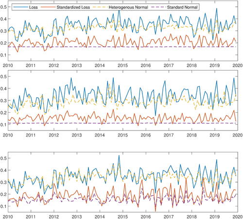
Like in Figure 4, we observe in Figure 5, a dramatic reduction in the estimated EVIs after standardization in every month. This suggests that the scale heterogeneity across individuals, rather than the GARCH residuals, generates the empirical power law here. To illustrate that the heterogeneity effect is dominant, we simulate heterogeneous normal variables with the calibrated GARCH variances from the cross-section for each period independently. We also generate independent standard normal variables for comparison. We plot the average of the Hill estimates for these normal variables (dotted yellow and dotted purple, respectively) over 100 replications in the figure as well. Their resemblance to the estimated EVIs of the stock losses is striking, especially when the thresholds are adaptive to monthly databases. In particular, as predicted by our asymptotic theory, the heterogeneous Gaussian model shows a much heavier tail than the homogeneous Gaussian model. Since every individual Gaussian variable is light-tailed, the power law is clearly generated by the scale heterogeneity.

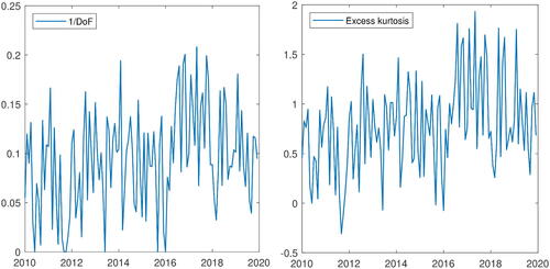
For robustness check, we repeat our residual calibration with the Student-t distribution rather than the Gaussian distribution. We fit a location-scale t-distribution to the GARCH residuals every month and plot the inverse of the degrees of freedom in Figure 6. In the same figure, we also plot the monthly sample excess kurtosis of the (pooled) GARCH residuals which are almost always positive with an average value of 0.7798. The inverse of the degrees of freedom increases with the kurtosis in general, with a correlation of more than 96%. We typically observe large degrees of freedom around 10, that is, with an inverse value around 0.1 like in Bollerslev and Wooldridge (1992). The degrees of freedom are sometimes very large (that is, its inverse value is close to zero) when the excess kurtosis is small, yielding similar results as for the Gaussian calibrations in those months.

Fig. 6 Monthly time series of the inverse of calibrated degrees of freedom (left) and sample kurtosis (right). The sample correlation between the time series is 0.9649.

We then simulate heterogeneous Student variables with the calibrated GARCH variances and the fitted degrees of freedom from the cross-section for each period independently. We also generate independent, homogeneous Student variables from the fitted distribution for comparison. We plot the average of the Hill estimates for these Student variables (dotted yellow and dotted purple, respectively) over 100 replications in Figure 7. Using the t-distribution improves the calibration for the naive choices of k equal to 5% and 1% of the sample size, and produces similar results as the Gaussian distribution for the adaptive choice of k. In all cases, we observe that the heterogeneous models generate a much heavier tail than the homogeneous models.

Fig. 7 Time series of estimated extreme value indices. The solid lines are for nominal stock losses (blue) and standardized stock losses (red). The dotted lines are for the calibrated heterogeneous Student-t variables (yellow) and the homogeneous Student-t variables (purple). The choices of k from top to the bottom are: top 5% of positive data, top 1% of positive data, and the adaptive choice suggested in Clauset, Shalizi, and Newman (2009).

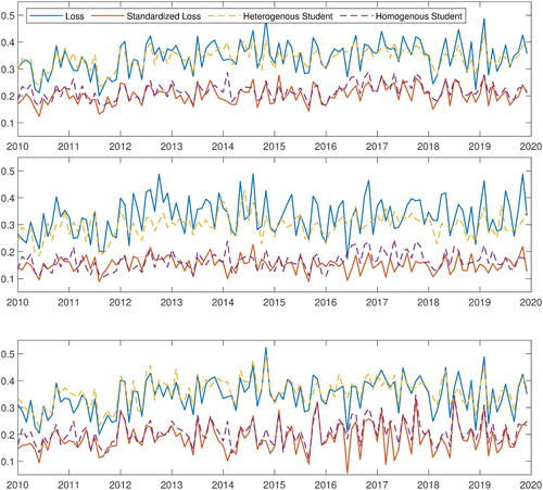
To summarize, our theory reveals that the cross-sectional volatility heterogeneity can generate empirical power laws across stock losses even if the residuals are relatively light tailed. One may consider such heavy tails to be spurious in the sense that they are not related to rare events of risk variables. We alert empirical researchers to these peculiar effects by presenting the much smaller estimates of the cross-sectional EVIs using volatility-standardized losses.

Acknowledgments

We thank the editor, Professor Christian Hansen, an Associate Editor, and two reviewers for their useful comments that led to this improved version of the article. John Einmahl holds the Arie Kapteyn Chair 2019–2022 and gratefully acknowledges the corresponding research support.

Supplementary Material

We provide the replication code in the online supplementary material.

Appendix.

Proofs

Proof of Theorem 1.

Define $b_p=\frac{\sqrt{k}}{p\sqrt{\hspace{0.17em}\text{log}\hspace{0.17em}p}}$ and consider$$\begin{array}{c}\frac{1}{k}\sum _{i=0}^{\lfloor p{b}_p\rfloor }\hspace{0.17em}\text{log}\hspace{0.17em}{X}_{p-i:p}-\hspace{0.17em}\text{log}\hspace{0.17em}{X}_{p-k:p}\le \frac{\lfloor p{b}_p\rfloor +1}{k}(\hspace{0.17em}\text{log}\hspace{0.17em}{X}_{p:p}-\hspace{0.17em}\text{log}\hspace{0.17em}{X}_{p-k:p})\\ \hspace{1em}=O_{\mathbb{P}}\left(\frac{1}{k}\frac{\sqrt{k}}{\sqrt{\hspace{0.17em}\text{log}\hspace{0.17em}p}}\text{log}\hspace{0.17em}p\right)=o_{\mathbb{P}}(1).\end{array}$$

Write $Y_i^{(p)}=\frac{1}{1-F(X_i^{(p)})}$. Then $X_i^{(p)}=U(Y_i^{(p)})$, with the function $U={(\frac{1}{1-F})}^{-1}$. Let $Y_{j:p},j=1,\dots ,p$ be the order statistics of the $Y_i^{(p)}$. By Assumptions 1 and 2, we have that $Y_{p-k:p}\stackrel{\mathbb{P}}{\to }\infty$. Now, as in the proof of Theorem 3.2.2 (the consistency of the Hill estimator in the iid case) in de Haan and Ferreira (2006), it suffices to prove that, as $p\to \infty$,(A.1) $$\frac{1}{k}\sum _{i=\lfloor p{b}_p\rfloor +1}^{k-1}\hspace{0.17em}\text{log}\hspace{0.17em}\frac{Y_{p-i:p}}{Y_{p-k:p}}\stackrel{\mathbb{P}}{\to }1.$$(A.1)

Let G_p be the empirical df of the $Y_i^{(p)},i=1,\dots ,p$. Then Assumption 1 implies for $\delta >0$ (A.2) $$\underset{F(c)+\delta \le u\le 1-2a_p}{\sup }\left|(1-u)G_p^{-1}(u)-1\right|\stackrel{\mathbb{P}}{\to }0.$$(A.2)

Let $\epsilon >0$. Then with probability tending to 1, we have from (A.2)(A.2) $$\underset{F(c)+\delta \le u\le 1-2a_p}{\sup }\left|(1-u)G_p^{-1}(u)-1\right|\stackrel{\mathbb{P}}{\to }0.$$(A.2) with $a_p\le \frac{1}{2}{b}_p$ (and $p{a}_p\to \infty$)$$\begin{array}{c}-\epsilon +\frac{1}{k}\sum _{i=\lfloor p{b}_p\rfloor +1}^{k-1}\hspace{0.17em}\text{log}\hspace{0.17em}\frac{k}{i}\le \frac{1}{k}\sum _{i=\lfloor p{b}_p\rfloor +1}^{k-1}\hspace{0.17em}\text{log}\hspace{0.17em}\frac{Y_{p-i:p}}{Y_{p-k:p}}\\ \hspace{1em}\le \epsilon +\frac{1}{k}\sum _{i=\lfloor p{b}_p\rfloor +1}^{k-1}\hspace{0.17em}\text{log}\hspace{0.17em}\frac{k}{i}.\end{array}$$

It is elementary to show that $\frac{1}{k}{\sum }_{i=\lfloor p{b}_p\rfloor +1}^{k-1}\hspace{0.17em}\text{log}\hspace{0.17em}\frac{k}{i}\to 1$. This yields (A.1)(A.1) $$\frac{1}{k}\sum _{i=\lfloor p{b}_p\rfloor +1}^{k-1}\hspace{0.17em}\text{log}\hspace{0.17em}\frac{Y_{p-i:p}}{Y_{p-k:p}}\stackrel{\mathbb{P}}{\to }1.$$(A.1) . □

Proof of Theorem 2.

Reshuffle the indices i such that the positive $c_{p,i}$ have a lower index than the $c_{p,i}$ equal to 0 and let κ_p be the number of positive $c_{p,i},i=1,\dots p$. Let $U_i=1-F_{p,i}(X_i^{(p)})$. Then the U_i are independent uniform-(0,1) random variables, and$$\begin{array}{c}1-F_{\text{emp}}(x)=\frac{1}{p}\sum _{i=1}^{p}1\left(X_i^{(p)}>x\right)\\ =\frac{1}{p}\sum _{i=1}^{p}1\left(U_i<1-F_{p,i}(x)\right)\\ =\frac{1}{p}\sum _{i=1}^{{\kappa }_p}1\left(U_i<1-F_{p,i}(x)\right)\\ \hspace{1em}+\frac{1}{p}\sum _{i={\kappa }_p+1}^{p}1\left(U_i<1-F_{p,i}(x)\right).\end{array}$$

Let $\eta >0$. For $i>{\kappa }_p$ and $x\ge c$ (for some large c), we have$$1-F_{p,i}(x)\le \eta \left(1-F(x)\right),$$and hence$$\begin{array}{c}\frac{1}{p}\sum _{i={\kappa }_p+1}^{p}1\left(U_i<1-F_{p,i}(x)\right)\\ \hspace{1em}\le \frac{1}{p}\sum _{i={\kappa }_p+1}^{p}1\left(U_i<\eta \left(1-F(x)\right)\right).\end{array}$$

Define ${\Gamma }_p(y)=\frac{1}{p}{\sum }_{i=1}^{p}1(U_i\le y)$, the uniform empirical df. Then$$\begin{array}{c}\frac{\frac{1}{p}\sum _{i={\kappa }_p+1}^{p}1\left(U_i<1-F_{p,i}(x)\right)}{1-F(x)}\\ \hspace{1em}\le \frac{{\Gamma }_p\left(\eta (1-F(x))\right)}{1-F(x)},\hspace{1em}\text{for} x\ge c.\end{array}$$

Using (Wellner 1978, theor. 0), we obtain that with probability tending to 1, as $p\to \infty$,$$\underset{c\le x\le Q(1-a_p)}{\sup }\frac{{\Gamma }_p(\eta (1-F(x)))}{\eta (1-F(x))}·\eta \le 2\eta .$$

Since $\eta >0$ can be made arbitrarily small, it remains to show that(A.3) $$\underset{c\le x\le Q(1-a_p)}{\sup }\left|\frac{\frac{1}{p}\sum _{i=1}^{{\kappa }_p}1\left(U_i<1-F_{p,i}(x)\right)}{1-F(x)}-1\right|\stackrel{\mathbb{P}}{\to }0.$$(A.3)

Let $\epsilon \in (0,1/(2d))$, where $d=\underset{p}{\sup }{\max }_{1\le i\le p}{c}_{p,i}\in (0,\infty )$.

Let B_i , $i=1,\dots ,{\kappa }_p$, be independent Bernoulli random variables with $\mathbb{P}(B_i=1)=c_{p,i}\epsilon$. Write $N_p={\sum }_{i=1}^{{\kappa }_p}{B}_i$. Let V_j , $j=1,\dots ,{\kappa }_p$, be independent uniform variables on (0, 1), independent of the B_i ’s. Pair the B_i and V_j in the following way: assign the first N_p , V_j to the B_i which are equal to 1 (and the other V_j to the B_i which are 0). Define$$U_i=B_i{c}_{p,i}\epsilon V_j+\left(1-B_i\right)\left[c_{p,i}\epsilon +(1-c_{p,i}\epsilon )V_j\right].$$

Then $U_1,\dots ,U_{{\kappa }_p}$ are independent uniform variables on (0, 1). (These U_i are different from those in (A.3)(A.3) $$\underset{c\le x\le Q(1-a_p)}{\sup }\left|\frac{\frac{1}{p}\sum _{i=1}^{{\kappa }_p}1\left(U_i<1-F_{p,i}(x)\right)}{1-F(x)}-1\right|\stackrel{\mathbb{P}}{\to }0.$$(A.3) , but since we consider only convergence in probability that is allowed.) Let $\delta >0$. For x large, since $\underset{p}{\inf }{\min }_{1\le i\le {\kappa }_p}{c}_{p,i}>0$,(A.4) $$\begin{array}{c}\frac{1}{p}\sum _{i=1}^{{\kappa }_p}1\left(U_i<(1-F(x))c_{p,i}(1-\delta )\right)\\ \hspace{1em}\le \frac{1}{p}\sum _{i=1}^{{\kappa }_p}1\left(U_i<(1-F_{p,i}(x))\right)\\ \hspace{1em}\le \frac{1}{p}\sum _{i=1}^{{\kappa }_p}1\left(U_i<(1-F(x))c_{p,i}(1+\delta )\right).\end{array}$$(A.4)

Write ${\tilde{\Gamma }}_m(y)=\frac{1}{m}{\sum }_{j=1}^{m}1(V_j\le y),m=1,\dots ,{\kappa }_p$. Now we have, for either choice of sign, for large x,$$\begin{array}{c}\frac{1}{p}\sum _{i=1}^{{\kappa }_p}1\left(U_i<(1-F(x))c_{p,i}(1\pm \delta )\right)\\ \hspace{1em}=\frac{1}{p}\sum _{j=1}^{N_p}1\left[V_j<(1-F(x))(1\pm \delta )/\epsilon \right]\\ \hspace{1em}=\frac{N_p}{p}{\tilde{\Gamma }}_{N_p}\left((1-F(x))(1\pm \delta )/\epsilon \right).\end{array}$$

Hence, for large x, the ratio in (A.3)(A.3) $$\underset{c\le x\le Q(1-a_p)}{\sup }\left|\frac{\frac{1}{p}\sum _{i=1}^{{\kappa }_p}1\left(U_i<1-F_{p,i}(x)\right)}{1-F(x)}-1\right|\stackrel{\mathbb{P}}{\to }0.$$(A.3) can be bounded from below/above by$$\frac{{\tilde{\Gamma }}_{N_p}((1-F(x))(1\pm \delta )/\epsilon )}{\frac{p}{N_p}(1-F(x))}=:R_{p,\pm }(x).$$

Clearly $\frac{E{N}_p}{p}=\frac{1}{p}{\sum }_{i=1}^{{\kappa }_p}{c}_{p,i}\epsilon \to \epsilon$. Now by the law of large numbers and again in (Wellner 1978, theor. 0), we have that$$\underset{c\le x\le Q(1-a_p)}{\sup }|R_{p,\pm }-1|\stackrel{\mathbb{P}}{\to }\delta .$$

Since $\delta >0$ is arbitrary, this in combination with (A.4)(A.4) $$\begin{array}{c}\frac{1}{p}\sum _{i=1}^{{\kappa }_p}1\left(U_i<(1-F(x))c_{p,i}(1-\delta )\right)\\ \hspace{1em}\le \frac{1}{p}\sum _{i=1}^{{\kappa }_p}1\left(U_i<(1-F_{p,i}(x))\right)\\ \hspace{1em}\le \frac{1}{p}\sum _{i=1}^{{\kappa }_p}1\left(U_i<(1-F(x))c_{p,i}(1+\delta )\right).\end{array}$$(A.4) yields (A.3)(A.3) $$\underset{c\le x\le Q(1-a_p)}{\sup }\left|\frac{\frac{1}{p}\sum _{i=1}^{{\kappa }_p}1\left(U_i<1-F_{p,i}(x)\right)}{1-F(x)}-1\right|\stackrel{\mathbb{P}}{\to }0.$$(A.3) .

The stability condition follows from$$Q_{p,i}(t)\le Q(1-(1-t)/(2d)),\hspace{1em}{t}_0\le t<1,\mathrm{ }\text{for}\mathrm{ }\text{some}\mathrm{ }{t}_0,$$and the asymptotic behavior of the minimum of p independent uniform-(0,1) random variables. □

Proof of Theorem 3.

Without loss of generality, we may and will assume μ = 0.

Let $U_1,\dots ,U_p$ be iid uniform-(0,1) random variables and denote their order statistics by $U_{1:p}\le \cdots \le U_{p:p}$. Let $Z_1,\dots ,Z_p$ be i.i.d. random variables from the df G and independent of the U_i . Consider the empirical survival functions$$\begin{array}{c}{S}_p(x):=\frac{1}{p}\sum _{i=1}^{p}1\left(Q_{\sigma }(U_i)Z_i>x\right)\mathrm{ }\text{and}\mathrm{ }\\ {\tilde{S}}_p(x):=\frac{1}{p}\sum _{i=1}^{p}1\left(Q_{\sigma }(U_{i:p})Z_i>x\right),x\in \mathbb{R}.\end{array}$$

Note that the $Q_{\sigma }(U_i)Z_i$ are iid with df F as in the theorem. Also observe that ${\tilde{S}}_p\stackrel{d}{=}{S}_p$ by the exchangeability of the Z_i and the independence of the U_i and the Z_i .

By (Wellner 1978, theor. 0), for any intermediate sequence $a=a(p)\to 0$ such that $pa\to \infty$,(A.5) $$\underset{x\le Q(1-a)}{\sup }\left|\frac{{\tilde{S}}_p(x)}{1-F(x)}-1\right|\stackrel{d}{=}\underset{x\le Q(1-a)}{\sup }\left|\frac{S_p(x)}{1-F(x)}-1\right|\stackrel{\mathbb{P}}{\to }0.$$(A.5)

We need to show a similar result, namely(A.6) $$\underset{c\le x\le Q(1-a)}{\sup }\left|\frac{1-F_{\text{emp}}(x)}{1-F(x)}-1\right|\stackrel{\mathbb{P}}{\to }0.$$(A.6)

We first show(A.7) $$\underset{1\le i\le (1-b)p}{\sup }\left|\frac{Q_{\sigma }(U_{i:p})}{Q_{\sigma }(i/p)}-1\right|\stackrel{\mathbb{P}}{\to }0.$$(A.7) where $b=b(p)\to 0$ is such that $b/a\to 0$ and $pb\to \infty$. The Glivenko–Cantelli theorem yields$$\underset{1\le i\le p}{\sup }\left|U_{i:p}-i/p\right|\stackrel{\mathbb{P}}{\to }0.$$

From this result, we obtain the convergence in (A.7)(A.7) $$\underset{1\le i\le (1-b)p}{\sup }\left|\frac{Q_{\sigma }(U_{i:p})}{Q_{\sigma }(i/p)}-1\right|\stackrel{\mathbb{P}}{\to }0.$$(A.7) for the supremum over $1\le i\le (1-t^{+})p$, by the (uniform) continuity of $Q_{\sigma }$ on $(0,1-t^{+}]$ and $Q_{\sigma }(0+)>0$. (Wellner 1978, theor. 0) also states that(A.8) $$\underset{1\le i\le (1-b)p}{\sup }\left|\frac{1-U_{i:p}}{1-i/p}-1\right|\stackrel{\mathbb{P}}{\to }0.$$(A.8)

Using this in combination with (3.1)(3.1) $$\underset{\delta \downarrow 0}{\lim }\underset{0<t\le t^{+},|s/t-1|\le \delta }{\sup }|Q_{\sigma }(1-s)/Q_{\sigma }(1-t)-1|=0.$$(3.1) , we obtain the convergence in (A.7)(A.7) $$\underset{1\le i\le (1-b)p}{\sup }\left|\frac{Q_{\sigma }(U_{i:p})}{Q_{\sigma }(i/p)}-1\right|\stackrel{\mathbb{P}}{\to }0.$$(A.7) for the supremum over $p(1-t^{+})\le i\le (1-b)p$. Clearly, by the first assumption of the model, (A.7)(A.7) $$\underset{1\le i\le (1-b)p}{\sup }\left|\frac{Q_{\sigma }(U_{i:p})}{Q_{\sigma }(i/p)}-1\right|\stackrel{\mathbb{P}}{\to }0.$$(A.7) implies(A.9) $$\underset{1\le i\le (1-b)p}{\sup }\left|\frac{Q_{\sigma }(U_{i:p})}{{\sigma }_{p,i}}-1\right|\stackrel{\mathbb{P}}{\to }0.$$(A.9)

Now decompose$$\begin{array}{c}1-F_{\text{emp}}(x)=\frac{1}{p}\sum _{i=1}^{p-\lfloor pb\rfloor }1\left({\sigma }_{p,i}{Z}_i>x\right)\\ \hspace{1em}+\frac{1}{p}\sum _{i=p-\lfloor pb\rfloor +1}^{p}1\left({\sigma }_{p,i}{Z}_i>x\right)\\ =:{\widehat{S}}_p^{(1)}(x)+{\widehat{S}}_p^{(2)}(x).\end{array}$$

Note that$$\underset{c\le x\le Q(1-a)}{\sup }\frac{{\widehat{S}}_p^{(2)}(x)}{1-F(x)}\le \frac{b}{a}\to 0.$$

Hence for (A.6)(A.6) $$\underset{c\le x\le Q(1-a)}{\sup }\left|\frac{1-F_{\text{emp}}(x)}{1-F(x)}-1\right|\stackrel{\mathbb{P}}{\to }0.$$(A.6) , it remains to show that(A.10) $$\underset{c\le x\le Q(1-a)}{\sup }\left|\frac{{\widehat{S}}_p^{(1)}(x)}{1-F(x)}-1\right|\stackrel{\mathbb{P}}{\to }0.$$(A.10)

Similarly, we can decompose$$\begin{array}{c}{\tilde{S}}_p(x)=\frac{1}{p}\sum _{i=1}^{p-\lfloor pb\rfloor }1\left(Q_{\sigma }(U_{i:p})Z_i>x\right)\\ \hspace{1em}+\frac{1}{p}\sum _{i=p-\lfloor pb\rfloor +1}^{p}1\left(Q_{\sigma }(U_{i:p})Z_i>x\right)\\ =:{\tilde{S}}_p^{(1)}(x)+{\tilde{S}}_p^{(2)}(x).\end{array}$$

Let $\epsilon \in (0,1)$. Recalling (A.9)(A.9) $$\underset{1\le i\le (1-b)p}{\sup }\left|\frac{Q_{\sigma }(U_{i:p})}{{\sigma }_{p,i}}-1\right|\stackrel{\mathbb{P}}{\to }0.$$(A.9) , with probability tending to 1, for all x > 0$${\tilde{S}}_p^{(1)}((1+\epsilon )x)\le {\widehat{S}}_p^{(1)}(x)\le {\tilde{S}}_p^{(1)}((1-\epsilon )x).$$

For ${\tilde{S}}_p^{(2)}$ we use again $b/a\to 0$. Hence, for (A.10)(A.10) $$\underset{c\le x\le Q(1-a)}{\sup }\left|\frac{{\widehat{S}}_p^{(1)}(x)}{1-F(x)}-1\right|\stackrel{\mathbb{P}}{\to }0.$$(A.10) , it suffices to show that, for either choice of sign, with probability tending to 1, for some N > 0 and small $\epsilon >0$ $$\underset{c\le x\le Q(1-a)}{\sup }\left|\frac{{\tilde{S}}_p((1\pm \epsilon )x)}{1-F(x)}-1\right|\le N\epsilon .$$

For either choice of sign,$$\begin{array}{c}\left|\frac{{\tilde{S}}_p((1\pm \epsilon )x)}{1-F(x)}-1\right|\le \left|\frac{{\tilde{S}}_p((1\pm \epsilon )x)}{1-F((1\pm \epsilon )x)}-1\right|\frac{1-F((1\pm \epsilon )x)}{1-F(x)}\\ +\left|\frac{1-F((1\pm \epsilon )x)}{1-F(x)}-1\right|.\end{array}$$

Recall from (A.5)(A.5) $$\underset{x\le Q(1-a)}{\sup }\left|\frac{{\tilde{S}}_p(x)}{1-F(x)}-1\right|\stackrel{d}{=}\underset{x\le Q(1-a)}{\sup }\left|\frac{S_p(x)}{1-F(x)}-1\right|\stackrel{\mathbb{P}}{\to }0.$$(A.5) that, with probability tending to 1,$$\underset{c\le x\le Q(1-a)}{\sup }\left|\frac{{\tilde{S}}_p((1\pm \epsilon )x)}{1-F((1\pm \epsilon )x)}-1\right|\le \underset{x\le Q(1-a\prime )}{\sup }\left|\frac{{\tilde{S}}_p(x)}{1-F(x)}-1\right|\stackrel{\mathbb{P}}{\to }0,$$where $a\prime =1-F((1+\epsilon )Q(1-a))$ is again an intermediate sequence as the regular variation of F implies that $a\prime /a\to {(1+\epsilon )}^{-\frac{1}{\gamma }}\in (0,\infty )$. Furthermore, by Potter (1942), it readily follows that that there exists an $\tilde{N}>0$, not depending on ε, such that$$\underset{c\le x\le Q(1-a)}{\sup }\left|\frac{1-F((1\pm \epsilon )x)}{1-F(x)}-1\right|\le \tilde{N}\epsilon$$ for some c > 0. As $\epsilon >0$ can be made arbitrarily small, we obtain (A.10) and hence (A.6).

For the stability condition, we have for large enough M,$$\begin{array}{c}\mathbb{P}(X_{p:p}>p^M)\le \mathbb{P}({\max }_{1\le i\le p}{Z}_i>p^M/{\sigma }_{p,p})\le \mathbb{P}({\max }_{1\le i\le p}{Z}_i>p^{M-1/\alpha })\\ \hspace{1em}=1-G^p(p^{M-1/\alpha })\le 1-{(1-p^{1-M\alpha })}^p\le p^{2-M\alpha }\to 0,\end{array}$$as $p\to \infty$. □

Proof of Theorem 4.

This proof is somewhat similar to that of Theorem 3, except we need to control the perturbations using the weight function q. Again, let $U_1,\dots ,U_p$ be iid uniform-(0,1) random variables and denote their order statistics by $U_{1:p}\le \dots \le U_{p:p}$; also, let $Z_1,\dots ,Z_p$ be iid random variables from the df G and independent of the U_i . Consider the empirical survival functions$$\begin{array}{c}{S}_{p,\eta }(x):=\frac{1}{p}\sum _{i=1}^{p}1\left(Q_{\mu }(U_i)+\eta q(U_i)+Z_i>x\right),\\ {\tilde{S}}_{p,\eta }(x)=\frac{1}{p}\sum _{i=1}^{p}1\left(Q_{\mu }(U_{i:p})+\eta q(U_{i:p})+Z_i>x\right),x\in \mathbb{R}.\end{array}$$

Note that the $Q_{\mu }(U_i)+\eta q(U_i)+Z_i$ are iid with df $F_{(\eta )}$ (as defined just above the theorem). Also observe that ${\tilde{S}}_{p,\eta }\stackrel{d}{=}{S}_{p,\eta }$ by the exchangeability of the Z_i and the independence of the U_i and Z_i .

Choose another sequence $b=b(p)$ with $b/a\to 0$ and $pb\to \infty$ and write$$\begin{array}{c}1-F_{\text{emp}}(x)=\frac{1}{p}\sum _{i=1}^{\lfloor pb\rfloor }1\left({\mu }_{p,i}+Z_i>x\right)\\ \mathrm{\hspace{1em}}\mathrm{\hspace{1em}}+\frac{1}{p}\sum _{i=\lfloor pb\rfloor +1}^{p-\lfloor pb\rfloor }1\left({\mu }_{p,i}+Z_i>x\right)\\ \mathrm{\hspace{1em}}\mathrm{\hspace{1em}}+\frac{1}{p}\sum _{i=p-\lfloor pb\rfloor +1}^{p}1\left({\mu }_{p,i}+Z_i>x\right)\\ \hspace{1em}=: {\widehat{S}}_p^{(1)}(x)+{\widehat{S}}_p^{(2)}(x)+{\widehat{S}}_p^{(3)}(x).\end{array}$$

Observe that $\underset{x\le Q(1-a)}{\sup }\frac{{\widehat{S}}_p^{(1)}(x)}{1-F(x)}\le \frac{b}{a}\to 0$ and $\underset{x\le Q(1-a)}{\sup }\frac{{\widehat{S}}_p^{(3)}(x)}{1-F(x)}\le \frac{b}{a}\to 0$. Hence for Chang’s condition it suffices to show that(A.11) $$\underset{c\le x\le Q(1-a)}{\sup }\left|\frac{{\widehat{S}}_p^{(2)}(x)}{1-F(x)}-1\right|\stackrel{\mathbb{P}}{\to }0.$$(A.11)

Now recall (A.8)(A.8) $$\underset{1\le i\le (1-b)p}{\sup }\left|\frac{1-U_{i:p}}{1-i/p}-1\right|\stackrel{\mathbb{P}}{\to }0.$$(A.8) and note that $(1-U_{1:p},\dots ,1-U_{p:p})\stackrel{d}{=}(U_{p:p},\dots ,U_{1:p})$. Using conditions (ii) and (iii),$$\begin{array}{c}{\max }_{pb\le i\le p(1-b)}\frac{\left|Q_{\mu }(U_{i:p})-Q_{\mu }(i/p)\right|}{q(i/p)}\stackrel{\mathbb{P}}{\to }0\mathrm{ }\text{and}\mathrm{ }\\ {\max }_{pb\le i\le p(1-b)}\frac{\left|q(U_{i:p})-q(i/p)\right|}{q(i/p)}\stackrel{\mathbb{P}}{\to }0.\end{array}$$

It follows that$$\begin{array}{c}\frac{|{\mu }_{p,i}-Q_{\mu }(U_{i:p})|}{q(U_{i:p})}\le \frac{|{\mu }_{p,i}-Q_{\mu }(i/p)|}{q(i/p)}\frac{q(i/p)}{q(U_{i:p})}\\ \hspace{1em}+\frac{|Q_{\mu }(U_{i:p})-Q_{\mu }(i/p)|}{q(i/p)}\frac{q(i/p)}{q(U_{i:p})}=o_{\mathbb{P}}(1),\end{array}$$uniformly for $pb\le i\le p(1-b)$. Hence, for any $\delta >0$, with probability tending to one,(A.12) $$\frac{{\tilde{S}}_{p,-\delta }\left(x\right)}{1-F(x)}-\frac{2b}{a}\le \frac{{\widehat{S}}_p^{(2)}(x)}{1-F(x)}\le \frac{{\tilde{S}}_{p,\delta }\left(x\right)}{1-F(x)},$$(A.12) uniformly for $c\le x\le Q(1-a)$, where for the first inequality we decompose ${\tilde{S}}_{p,-\delta }$ like $1-F_{\text{emp}}$ above. For either choice of sign,$$\begin{array}{c}\left|\frac{{\tilde{S}}_{p,\pm \delta }(x)}{1-F(x)}-1\right|\le \left|\frac{{\tilde{S}}_{p,\pm \delta }(x)}{1-F_{(\pm \delta )}(x)}-1\right|\left|\frac{1-F_{(\pm \delta )}(x)}{1-F(x)}\right|\\ \hspace{1em}+\left|\frac{1-F_{(\pm \delta )}(x)}{1-F(x)}-1\right|.\end{array}$$

Let $\epsilon \in (0,\frac{1}{2})$. Note that by condition (i), we have that, there exists a ${\delta }_1>0$ such that for $0<\delta \le {\delta }_1$ and either choice of sign,(A.13) $$\underset{c\le x}{\sup }\left|\frac{1-F_{(\pm \delta )}(x)}{1-F(x)}-1\right|\le \epsilon .$$(A.13)

Furthermore, by (Wellner 1978, theor. 0), for either choice of sign,(A.14) $$\underset{x\le Q(1-a)}{\sup }\left|\frac{{\tilde{S}}_{p,\pm \delta }(x)}{1-F_{(\pm \delta )}(x)}-1\right|\stackrel{d}{=}\underset{x\le Q(1-a)}{\sup }\left|\frac{S_{p,\pm \delta }(x)}{1-F_{(\pm \delta )}(x)}-1\right|\stackrel{\mathbb{P}}{\to }0,$$(A.14) as $1-F_{(\pm \delta )}(Q(1-a))$ is again an intermediate sequence, by (A.13). Hence, with probability tending to 1,$$\underset{c\le x\le Q(1-a)}{\sup }\left|\frac{{\tilde{S}}_{p,\pm \delta }(x)}{1-F(x)}-1\right|\le 2\epsilon .$$

Combining this with (A.12)(A.12) $$\frac{{\tilde{S}}_{p,-\delta }\left(x\right)}{1-F(x)}-\frac{2b}{a}\le \frac{{\widehat{S}}_p^{(2)}(x)}{1-F(x)}\le \frac{{\tilde{S}}_{p,\delta }\left(x\right)}{1-F(x)},$$(A.12) and recalling that $b/a\to 0$, we obtain (A.11)(A.11) $$\underset{c\le x\le Q(1-a)}{\sup }\left|\frac{{\widehat{S}}_p^{(2)}(x)}{1-F(x)}-1\right|\stackrel{\mathbb{P}}{\to }0.$$(A.11) .

The proof of the stability condition is straightforward using $X_p^{(p)}\le {\mu }_{p,p}+{\max }_{1\le i\le p}{Z}_i$. □

Proof of Theorem 5.

Let $F_{p,t}$ denote the empirical df of the subsample corresponding to a fixed $t\in \{1,\dots ,T\}$. Observe that $F_{\text{emp}}$ is a convex combination of the $F_{p,t}$ with weights $p_t/p$, that is,$$F_p(x)=\sum _{t=1}^T\frac{p_t}{p}{F}_{p,t}(x), x\in \mathbb{R}.$$

Recall that $F(x)=\sum _{t\in {\mathcal{T}}_{\infty }}{w}_t{F}_t(x)$. Denote the generalized quantile function of F as Q and that of F_t as Q_t . Then$$\begin{array}{c}\left|\frac{1-F_{\text{emp}}(x)}{1-F(x)}-1\right|=\left|\sum _{t=1}^T\frac{p_t}{p}\frac{1-F_{p,t}(x)}{1-F(x)}-\sum _{t\in {\mathcal{T}}_{\infty }}{w}_t\frac{1-F_t(x)}{1-F(x)}\right|\\ \le \sum _{t\in {\mathcal{T}}_{\infty }}{w}_t\left|\frac{1-F_{p,t}(x)}{1-F(x)}-\frac{1-F_t(x)}{1-F(x)}\right|\\ +\sum _{t\notin {\mathcal{T}}_{\infty }}\frac{p_t}{p}\frac{1-F_{p,t}(x)}{1-F(x)}\\ +\sum _{t\in {\mathcal{T}}_{\infty }}\left|\frac{p_t}{p}-w_t\right|\frac{1-F_{p,t}(x)}{1-F(x)}\\ =:J_1(x)+J_2(x)+J_3(x).\end{array}$$

For any intermediate sequence $a=a(p)$,$$\underset{x\le Q(1-a)}{\sup }{J}_2(x)\le \sum _{t\notin {\mathcal{T}}_{\infty }}\frac{p_t}{pa}\to 0.$$

Now take another intermediate sequence $b=b(p)$ such that $b/a\to 0$. We have that$$\begin{array}{c}\underset{c\le x\le Q(1-a)}{\sup }{J}_1(x)\le \sum _{t\in {\mathcal{T}}_{\infty }}{w}_t\underset{c\le x\le \min \{Q_t(1-b),Q(1-a)\}}{\sup }\\ \hspace{1em}\left|\frac{1-F_{p,t}(x)}{1-F(x)}-\frac{1-F_t(x)}{1-F(x)}\right|\\ +\sum _{t\in {\mathcal{T}}_{\infty }}{w}_t\underset{\min \{Q_t(1-b),Q(1-a)\}\le x\le Q(1-a)}{\sup }\\ \hspace{1em}\left|\frac{1-F_{p,t}(x)}{1-F(x)}-\frac{1-F_t(x)}{1-F(x)}\right|\\ =:A_1+A_2.\end{array}$$

By the assumed Chang’s conditions for each $t\in {\mathcal{T}}_{\infty }$, we have for sufficiently large c,$$\begin{array}{c}{A}_1=\sum _{t\in {\mathcal{T}}_{\infty }}\underset{c\le x\le \min \{Q_t(1-b),Q(1-a)\}}{\sup }\left|\frac{1-F_{p,t}(x)}{1-F_t(x)}-1\right|·w_t\frac{1-F_t(x)}{1-F(x)}\\ \le {\max }_{t\in {\mathcal{T}}_{\infty }}\underset{c\le x\le \min \{Q_t(1-b),Q(1-a)\}}{\sup }\left|\frac{1-F_{p,t}(x)}{1-F_t(x)}-1\right|\stackrel{\mathbb{P}}{\to }0.\end{array}$$

On the other hand, again by the Chang’s conditions,$$\begin{array}{c}{A}_2\le \sum _{t\in {\mathcal{T}}_{\infty }}{w}_t·\frac{1}{a}\underset{\min \{Q_t(1-b),Q(1-a)\}\le x\le Q(1-a)}{\sup }\\ \hspace{1em}\left\{\left(1-F_{p,t}(x)\right)+\left(1-F_t(x)\right)\right\}\\ \le \sum _{t\in {\mathcal{T}}_{\infty }}\frac{w_t}{a}\left\{\left(1-F_{p,t}(Q_t(1-b))\right)+\left(1-F_t(Q_t(1-b))\right)\right\}\\ \le \sum _{t\in {\mathcal{T}}_{\infty }}\frac{w_{t}b}{a}\left\{\frac{1-F_{p,t}(Q_t(1-b))}{1-F_t(Q_t(1-b))}+1\right\}\\ \le {\max }_{t\in {\mathcal{T}}_{\infty }}\left|\frac{1-F_{p,t}(Q_t(1-b))}{1-F_t(Q_t(1-b))}+1\right|\sum _{t\in {\mathcal{T}}_{\infty }}\frac{w_{t}b}{a}\\ \le {\max }_{t\in {\mathcal{T}}_{\infty }}\left|\frac{1-F_{p,t}(Q_t(1-b))}{1-F_t(Q_t(1-b))}+1\right|·\frac{b}{a}=O_{\mathbb{P}}(1)·o(1)\stackrel{\mathbb{P}}{\to }0.\end{array}$$

Finally,$$\begin{array}{c}{J}_3(x)\le \sum _{t\in {\mathcal{T}}_{\infty }}\left|\frac{p_t}{p}-w_t\right|\left|\frac{1-F_{p,t}(x)}{1-F(x)}-\frac{1-F_t(x)}{1-F(x)}\right|\\ \hspace{1em}+\sum _{t\in {\mathcal{T}}_{\infty }}\left|\frac{p_t}{p}-w_t\right|\frac{1-F_t(x)}{1-F(x)}\\ \le {\max }_{t\in {\mathcal{T}}_{\infty }}\left|\frac{p_t}{p{w}_t}-1\right|·J_1(x)+{\max }_{t\in {\mathcal{T}}_{\infty }}\left|\frac{p_t}{p{w}_t}-1\right|\stackrel{\mathbb{P}}{\to }0,\end{array}$$uniformly for $c\le x\le Q(1-a)$.

The stability condition follows readily. □

References

- Allen, L., Bali, T. G., and Tang, Y. (2012), “Does Systemic Risk in the Financial Sector Predict Future Economic Downturns?” The Review of Financial Studies, 25, 3000–3036. DOI: 10.1093/rfs/hhs094.
- Atkinson, A. B. (2005), “Top Incomes in the UK Over the 20th Century,” Journal of the Royal Statistical Society, Series A, 168, 325–343. DOI: 10.1111/j.1467-985X.2005.00351.x.
- Axtell, R. L. (2001), “Zipf Distribution of U.S. Firm Sizes,” Science, 293, 1818–1820. DOI: 10.1126/science.1062081.
- Balkema, A. A., and de Haan, L. (1974), “Residual Life Time at Great Age,” The Annals of Probability, 2, 792–804. DOI: 10.1214/aop/1176996548.
- Barabási, A. L., and Albert, R. (1999), “Emergence of Scaling in Random Networks,” Science, 286, 509–512. DOI: 10.1126/science.286.5439.509.
- Barro, R. J., and Jin, T. (2011), “On the Size Distribution of Macroeconomic Disasters,” Econometrica, 79, 1567–1589.
- Bollerslev, T., and Wooldridge, J. M. (1992), “Quasi-Maximum Likelihood Estimation and Inference in Dynamic Models with Time-Varying Covariances,” Econometric Reviews, 11, 143–172. DOI: 10.1080/07474939208800229.
- Cao, W., and Zhang, Z. (2020), “New Extreme Value Theory for Maxima of Maxima,” Statistical Theory and Related Fields, DOI: 10.1080/24754269.2020.1846115.
- Chang, L. C. (1955), “On the Ratio of the Empirical Distribution Function to the Theoretical Distribution Function,” Acta Mathematica Sinica, 347–368; English translation: Selected Translations in Mathematical Statistics and Probability, vol. 4, American Mathematical Society, 1964, 17–38.
- Clauset, A., Shalizi, C., and Newman, M. (2009), “Power-Law Distributions in Empirical Data,” SIAM Review, 51, 661–703. DOI: 10.1137/070710111.
- Cont, R. (2001), “Empirical Properties of Asset Returns: Stylized Facts and Statistical Issues,” Quantitative Finance, 1, 223–236. DOI: 10.1080/713665670.
- di Giovanni, J., and Levchenko, A.A. (2012), “Country Size, International Trade, and Aggregate Fluctuations in Granular Economies,” Journal of Political Economy, 120, 1083–1132. DOI: 10.1086/669161.
- di Giovanni, J., Levchenko, A. A., and Rancière, R. (2011), “Power Laws in Firm Size and Openness to Trade: Measurement and Implications,” Journal of International Economics, 85, 42–52. DOI: 10.1016/j.jinteco.2011.05.003.
- Einmahl, J. H. J., de Haan, L., and Zhou, C. (2016), “Statistics of Heteroscedastic Extremes,” Journal of the Royal Statistical Society, Series B, 78, 31–51. DOI: 10.1111/rssb.12099.
- Embrechts, P., Klüppelberg, C., and Mikosch, T. (1997), Modelling Extremal Events: for Insurance and Finance, Berlin: Springer.
- Fagereng, A., Guiso, L. and Pistaferri, L. (2020), “Heterogeneity and Persistence in Returns to Wealth,” Econometrica, 88, 115–170. DOI: 10.3982/ECTA14835.
- Fama, E.F. (1963), “Mandelbrot and the Stable Paretian Hypothesis,” The Journal of Business, 36, 420–429. DOI: 10.1086/294633.
- Feller, W. (1978), An Introduction to Probability Theory and Its Applications, Vol. 2, New York: Wiley.
- Fisher, R. A., and Tippett, L.H.C. (1928), “Limiting Forms of the Frequency Distribution of the Largest or Smallest Member of a Sample,” Mathematical Proceedings of the Cambridge Philosophical Society, 24, 180–190. DOI: 10.1017/S0305004100015681.
- Fisk, P. R. (1961), “The Graduation of Income Distributions,” Econometrica, 29, 171–185. DOI: 10.2307/1909287.
- Gabaix, X. (1999), “Zipf’s Law for Cities: An Explanation,” Quarterly Journal of Economics, 114, 739–767. DOI: 10.1162/003355399556133.
- Gabaix, X. (2009), “Power Laws in Economics and Finance,” Annual Review of Economics, 1, 255–294.
- Gabaix, X. (2016), “Power Laws in Economics: An Introduction,” Journal of Economic Perspectives, 30, 185–206.
- Gabaix, X., Gopikrishnan, P., Plerou, V., and Stanley, H. E., “Institutional Investors and Stock Market Volatility,” The Quarterly Journal of Economics, 121, 461–504. DOI: 10.1162/qjec.2006.121.2.461.
- Gabaix, X., and Ioannides, Y. M. (2004), “The Evolution of City Size Distributions,” in Handbook of Regional and Urban Economics (Vol. 4), eds. V. Henderson and J.-F. Thisse, Amsterdam: Elsevier North-Holland, pp. 2341–2378.
- Gabaix, X., and Landier, A. (2008) “Why Has CEO Pay Increased so Much?” Quarterly Journal of Economics, 123, 49–100. DOI: 10.1162/qjec.2008.123.1.49.
- Gabaix, X., Lasry, J. M., Lions, P. L., and Moll, B. (2016), “The Dynamics of Inequality,” Econometrica, 84, 2071–2111. DOI: 10.3982/ECTA13569.
- Gardes, L. (2015), “A General Estimator for the Extreme Value Index: Applications to Conditional and Heteroscedastic Extremes,” Extremes, 18, 479–510. DOI: 10.1007/s10687-015-0220-6.
- Gnedenko, B. (1943), “Sur La Distribution Limite Du Terme Maximum D’Une Série Aléatoire,” Annals of Mathematics, 44, 423–453. DOI: 10.2307/1968974.
- Gopikrishnan, P., Plerou, V., Gabaix, X., and Stanley, H. E. (2000), “Statistical Properties of Share Volume Traded in Financial Markets,” Physical Review E, 62, R4493–R4496. DOI: 10.1103/physreve.62.r4493.
- Gopikrishnan, P., Plerou, V., Nunes Amaral, L. A., Meyer, M., and Stanley, H. E. (1999), “Scaling Of the Distribution of Fluctuations of Financial Market Indices,” Physical Review E, 60, 5305–5316. DOI: 10.1103/PhysRevE.60.5305.
- de Haan, L., and Ferreira, A. (2006), Extreme Value Theory: An Introduction, New York: Springer.
- Hill, B.M. (1975), “A Simple General Approach to Inference about the Tail of a Distribution,” The Annals of Statistics, 3, 1163–1174. DOI: 10.1214/aos/1176343247.
- Hüsler, J. (1986), “Extreme Values of Non-stationary Random Sequences,” Journal of Applied Probability, 23, 937–950. DOI: 10.2307/3214467.
- Jackson, M.O. (2009), “Networks and Economic Behavior,” Annual Review of Economics, 1, 489–511. DOI: 10.1146/annurev.economics.050708.143238.
- Jansen, D. W., and de Vries, C. G. (1991), “On the Frequency of Large Stock Returns: Putting Booms and Busts into Perspective,” The Review of Economics and Statistics, 73, 18–24. DOI: 10.2307/2109682.
- Jessen, A. H., and Mikosch, T. (2006), “Regularly Varying Functions,” Publications de l’Institut Mathematique, 80, 171–192. DOI: 10.2298/PIM0694171J.
- Kelly, B. (2014), “The Dynamic Power Law Model,” Extremes, 17, 557–583. DOI: 10.1007/s10687-014-0193-x.
- Kelly, B., and Jiang, H. (2014), “Tail Risk and Asset Prices,” The Review of Financial Studies, 27, 2841–2871. DOI: 10.1093/rfs/hhu039.
- Kyle, A.S., and Obizhaeva, A. A. (2016), “Market Microstructure Invariance: Empirical Hypotheses,” Econometrica, 84, 1345–1404. DOI: 10.3982/ECTA10486.
- Leadbetter, M.R., Lindgren, G., and Rootzén, H. (1983), Extremes and Related Properties of Random Sequences and Processes, New York: Springer.
- Longin, F.M. (1996), “The Asymptotic Distribution of Extreme Stock Market Returns,” The Journal of Business, 69, 383–408. DOI: 10.1086/209695.
- Mandelbrot, B. (1963), “The Variation of Certain Speculative Prices,” The Journal of Business, 36, 394–419. DOI: 10.1086/294632.
- Newman, M. E., Barabási, A. L. E., and Watts, D. J. (2006), The Structure and Dynamics of Networks, Princeton, NJ: Princeton University Press.
- Pareto, V. (1896), Cours d’Économie Politique, Lausanne: F. Rouge.
- Pickands, J. (1975), “Statistical Inference Using Extreme Order Statistics,” The Annals of Statistics, 3, 119–131.
- Piketty, T., and Goldhammer, A. (2014), Capital in the Twenty-First Century, Cambridge, MA: Harvard University Press.
- Piketty, T., and Saez, E. (2003), “Income Inequality in the United States,” Quarterly Journal of Economics, 118, 1–41. DOI: 10.1162/00335530360535135.
- Plerou, V., and Stanley, H. E. (2007), “Tests of Scaling and Universality of the Distributions of Trade Size and Share Volume: Evidence from Three Distinct Markets,” Physical Review E, 76, 046109. DOI: 10.1103/PhysRevE.76.046109.
- Potter, H. (1942), “The Mean Values of Certain DIrichlet Series, II,” Proceedings of the London Mathematical Society, 2, 1–19. DOI: 10.1112/plms/s2-47.1.1.
- Redner, S. (1998), “How Popular Is Your Paper? An Empirical Study of the Citation Distribution,” The European Physical Journal B-Condensed Matter and Complex Systems, 4, 131–134. DOI: 10.1007/s100510050359.
- Resnick, S. I. (2007), Heavy-tail Phenomena: Probabilistic and Statistical Modeling, New York: Springer.
- Schluter, C. (2021), “On Zipf’s Law and the Bias of Zipf Regressions,” Empirical Economics, 61, 529–548. DOI: 10.1007/s00181-020-01879-3.
- Stanley, M. H., Buldyrev, S. V., Havlin, S., Mantegna, R. N., Salinger, M. A., and Eugene Stanley, H. (1995), “Zipf Plots and the Size Distribution of Firms,” Economics Letters, 49, 453–457. DOI: 10.1016/0165-1765(95)00696-D.
- Toda, A. A., and Walsh, K. (2015), “The Double Power Law in Consumption and Implications For Testing Euler Equations”, Journal of Political Economy, 123, 1177–1200. DOI: 10.1086/682729.
- Wellner, J. A.(1978), “Limit Theorems for the Ratio of the Empirical Distribution Function to the True Distribution Function,” Zeitschrift für Wahrscheinlichkeitstheorie und Verwandte Gebiete, 45, 73–88. DOI: 10.1007/BF00635964.
- Zipf, G. K. (1949), Human Behavior and the Principle of Least Effort, Boston, MA: Addison Wesley Press
- Zucman, G. (2019), “Global Wealth Inequality,” Annual Review of Economics, 11, 109–138. DOI: 10.1146/annurev-economics-080218-025852.