Combining p-values for Multivariate Predictive Ability Testing

Abstract

In this article, we propose an intersection-union test for multivariate forecast accuracy based on the combination of a sequence of univariate tests. The testing framework evaluates a global null hypothesis of equal predictive ability using any number of univariate forecast accuracy tests under arbitrary dependence structures, without specifying the underlying multivariate distribution. An extensive Monte Carlo simulation exercise shows that our proposed test has very good size and power properties under several relevant scenarios, and performs well in both low- and high-dimensional settings. We illustrate the empirical validity of our testing procedure using a large dataset of 84 daily exchange rates running from January 1, 2011 to April 1, 2021. We show that our proposed test addresses inconclusive results that often arise in practice.

KEYWORDS:

• Exchange rates
• Forecasting evaluation
• Intersection-union tests
• Predictive Accuracy

1 Introduction

In this article, we propose a computationally efficient test for multivariate predictive ability that is valid for any number of univariate forecast accuracy tests and arbitrary dependence structures, without specifying the underlying multivariate distribution.

One of the main goals of econometric analysis is to make accurate predictions of a large range of variables such as inflation, exchange rates, stock returns, or volatility. To this purpose, there exist a large number of candidate models and the main challenge is to select the one with the best predictive ability. Thus far, the literature has proposed a variety of testing procedures, most of which are univariate and evaluate two competing forecasts of a single variable. Important examples include Diebold and Mariano (1995, DM) and Giacomini and White (2006, GW). [See Clark and McCracken (2013) for a comprehensive overview of existing testing procedures.] However, researchers are often interested in evaluating more than two forecasts, either because multivariate models are used (e.g., Laurent, Rombouts, and Violante 2013) or multiple variables are forecast (e.g., Carriero, Galvão, and Kapetanios 2019). In such cases, independence between variables and forecasting models seldom holds true. Consequently, univariate test statistics and their p-values can also exhibit dependencies, which means they cannot necessarily be evaluated individually. This motivates the development of multivariate forecast tests that account for dependence. Notably, the joint distribution of dependent variables is difficult or impossible to obtain analytically without several assumptions. The existing literature approaches this issue by evaluating a set of forecasts directly with a single test that adequately captures dependencies. For instance, Qu, Timmermann, and Zhu (in press) condition on a common factor within forecast errors to capture any common components. Mariano and Preve (2012) extend the DM test into a multivariate setting without directly addressing the dependence structure. However, approaches that evaluate forecasts jointly suffer from drawbacks that may render them infeasible in certain situations. First, their limiting framework is valid only under either a large or a small cross-section, restricting their applicability. That is, one cannot use the same test with datasets of considerably different dimensions. Second, the design of the forecasting scenario can require the use of multiple different tests, for example, because one compares nested and nonnested model or uses different estimation windows that affect the asymptotic properties of tests. Third, it is not always obvious when a test rejects in a multivariate setting in the sense that it is undefined how many individual forecasts must be equally accurate for the null to be sustained.

The testing framework we propose combines univariate tests, taking advantage of both recent advances in the statistical literature on combining dependent p-values as well as in the econometric literature on multivariate forecast evaluation. The resulting test allows researchers to estimate any number of univariate forecast accuracy tests—provided they fulfill some nonrestrictive assumptions—and corrects for dependence in a subsequent step that combines their p-values. Thus, one can implement tests that are most appropriate in a given scenario and examine whether predictive ability holds in the cross-section. We specify a global null hypothesis that is clearly defined as the intersection of all individual null hypotheses, accounting for false discovery and dependence. Furthermore, our method can be applied to p-values from different tests, meaning that when faced with mixed or inconclusive evidence, one can obtain a more conclusive result. Hence, our test can be used in a plethora of, if not all, forecasting scenarios. To the best of our knowledge, we are the first to propose such a test.

Specifically, we propose an intersection-union (IU) test by applying the theoretical results in Vovk and Wang (2020). We show that one can construct a global hypothesis test, based on a single or several of the existing univariate tests for forecast accuracy, that is level-α under any form of dependence. Crucially, our global test does not require knowledge of the joint distribution of the p-values of the individual test statistics which cannot be derived analytically. In addition, we study the power properties of the test and show under what conditions Type I and II errors vanish. We demonstrate the good size and power properties of the test through a battery of Monte Carlo simulations. For this purpose, we use three benchmark tests: DM, GW, and Clark and West (2007, CW). The three tests are widely used and suitable in different scenarios. However, we emphasize that our method is not restricted to these tests, meaning it can be deployed in a range of forecasting situations. The simulations evaluate the performance of our test in low-dimensional as well as high-dimensional scenarios. We compare our method to the Mariano and Preve (2012) test, a multivariate GW test, and methods that do not account for dependence between p-values. The simulations show that these procedures display considerable size distortions, effectively rendering them inapplicable in practical scenarios. When investigating their rejection accuracy, we find that contrary to our test, the other multivariate procedures, which are both of Wald-type, exhibit distinctly different rejection rates when dimensions change. This highlights how the interpretation of test results can benefit from our intersection null in practice. We illustrate the empirical validity of our testing procedure via an application involving a large dataset of 84 daily exchange rates, running from January 1, 2011 to April 1, 2021, quoted against the U.S.-Dollar, the British Pound, and the Euro. The empirical illustration highlights the wide-ranging applicability of our test both in small and high dimensional cases. Moreover, it exemplifies how our test addresses inconclusive results that arise often in practice.

The remainder of the article is structured as follows: Section 2 describes the forecasting setup, introduces the IU testing framework, and also reports a way to apply the GW test in a multivariate setting. Section 3 analyzes the size and power properties of the test in various simulations and Section 4 provides an empirical illustration of the test. Section 5 concludes.

2 Theory

This section presents our theoretical contribution. First, we outline a general framework for univariate forecast evaluation that is consistent with our test. Second, we propose treating univariate tests as subtests of a global null hypothesis and discuss the assumptions imposed upon them. Third, we introduce our methodology for multivariate forecast comparison which is based on the intersection of the subtests. Finally, we show how the Wald-type GW test can be applied in a multivariate setting and serve as a benchmark for our IU test.

2.1 Forecasting Setup

Suppose we observe the vector ${\mathit{V}}_t\equiv (Y{\prime }_t,X_t^{\prime })\prime$, where $Y=\{Y_t:\mathcal{Y}\mapsto {\mathbb{R}}^n,n\in \mathbb{N}\}$ are the variables one wishes to forecast and $X=\{X_t:\mathcal{X}\mapsto {\mathbb{R}}^s,s\in \mathbb{N}\}$ are predictor variables. Define ${\mathit{F}}_t$ as the σ-field generated by the infinite history of $\mathit{V}\equiv \{{\mathit{V}}_t:\Omega \mapsto {\mathbb{R}}^{s+n}\}$ and $\mathcal{Y}\cup \mathcal{X}=\Omega$ such that V is defined on the complete probability space $(\Omega ,\mathit{F},P)$. The forecasting equation for Y_t takes the form of an ${\mathit{F}}_t$-measurable function $\psi :\Omega \mapsto \mathcal{F}\subset \mathbb{R}$. The function can include lagged values of Y_t as well as X_t and can be parametric or nonparametric. It produces τ-step-ahead forecasts $\widehat{Y}=\{{\widehat{Y}}_{t+\tau }:\mathcal{F}\mapsto {\mathbb{R}}^n\}$ of Y based on the information set ${\mathit{F}}_t$. Notation-wise, we define the estimation window of the parameters as R and place no restrictions on whether R is a fixed, rolling, or expanding estimation window. Further, we define the out-of-sample forecasting window as p such that $T=R+p+\tau$ is the total sample the forecaster observes. Multiple procedures to evaluate the resulting forecasts have been introduced, most of which rely on a forecast loss function. The forecast loss function is defined as $L(\widehat{Y},Y,X):\mathcal{F}\times \Omega \mapsto \Lambda$. In many cases, the loss function is defined such that $\Lambda \subset {\mathbb{R}}_{+}$, with the most common type being the quadratic loss:$$L_{i,R,t+\tau }={\left(Y_{i,t+\tau }-{\widehat{Y}}_{i,t+\tau }\right)}^2,\hspace{1em}i\in \{1,\dots ,n\}.$$

The function can take many other forms and gives a vector ${\left\{L_{R,t+\tau }\right\}}_{t=R}^T$. One can assess forecasts based on a single loss function by testing whether it is statistically different from zero. For two forecasts, ${\widehat{Y}}^{(1)}$ and ${\widehat{Y}}^{(2)}$, one can define a loss differential, $\Delta L\equiv L({\widehat{Y}}^{(1)},Y,X)-L({\widehat{Y}}^{(2)},Y,X)$. That is, in the quadratic case we have$$\begin{array}{cc}\Delta L_{i,R,t+\tau }={\left(Y_{i,t+\tau }-{\widehat{Y}}_{i,t+\tau }^{(1)}\right)}^2-{\left(Y_{i,t+\tau }-{\widehat{Y}}_{i,t+\tau }^{(2)}\right)}^2,\hfill & \hfill \\ i\in \{1,\dots ,n\}.\hfill & \hfill \end{array}$$

The vector $\Delta {\mathit{L}}_{R,t+1}$ then stacks the n univariate loss differentials. Note that one can use several different loss functions to evaluate the same forecasts. However, the majority of existing forecast accuracy tests evaluate forecasts based on one single loss differential. Most commonly, by either formulating the unconditional null hypothesis ${\mathcal{H}}_{i,0}:\mathbb{E}[\Delta L_{i,R,t+\tau }]={\mu }_{i,0}$ or the conditional null ${\mathcal{H}}_{i,0}:\mathbb{E}[\Delta L_{i,R,t+\tau }|{\mathit{F}}_t]={\mu }_{i,0}$. The parameter ${\mu }_{i,0}$ is known and set to be zero when testing for equal predictive ability. The second type of tests is then called conditional equal predictive ability test and can ascertain if a particular model has superior forecasting abilities. This is a notable difference to unconditional tests that only assess if there are statistically significant differences between two forecasts. We use the notation of GW, $\mathbb{E}[\Delta L_{i,R,t+\tau }|{\mathit{G}}_t]={\mu }_i$, where ${\mathit{G}}_t$ corresponds to either the natural filtration ${\mathit{F}}_t$ or the trivial σ-field $\{\varnothing ,\Omega \}$, thereby referring to either of the two test types. The parameter μ_i characterizes either the unconditional or the conditional mean of the loss differential of the two forecasts. In this article, we consider the global null hypothesis:$${\mathcal{H}}_0:\mathbb{E}[\Delta {\mathit{L}}_{R,t+\tau }|{\mathit{G}}_t]={\mathit{\mu }}_0.$$

Constructing a test for this hypothesis is less straightforward. One approach is to construct a single test, based on the entire sample space Λ that jointly evaluates all elements in $\Delta {\mathit{L}}_{R,t+\tau }$. Dependencies between these elements pose an analytical and computational obstacle in the construction of a valid test. Therefore, we propose to test the intersection of the local hypotheses ${\mathcal{H}}_{i,0}$. Our methodology is compatible with all univariate test types that fulfill the assumptions outlined in the next section.

2.2 Univariate Subtests

Consider a series of n forecast accuracy tests, each of which is based on the random variables $Y_{i,t}$ and X_t. The tests all examine the local hypothesis ${\mathcal{H}}_{i,0}$, that is, compare the accuracy of two forecasts of the variable $Y_{i,t}$. We treat these tests as subtest for the global null hypothesis that all forecasts exhibit equal accuracy. Each univariate subtest evaluates the subhypothesis:$${\mathcal{H}}_{i,0}:{\mu }_i\in {\mathsf{M}}_{i,0},\mathrm{\hspace{1em}}\mathrm{\hspace{1em}}\text{for}i\in \{1,\dots ,n\},$$

against the alternative$${\mathcal{H}}_{i,A}:{\mu }_i\in {\mathsf{M}}_{i,A},\mathrm{\hspace{1em}}\mathrm{\hspace{1em}}\text{for}i\in \{1,\dots ,n\},$$where ${\mathsf{M}}_{i,0}$ is the set of admissible values for μ_i under the subhypothesis and ${\mathsf{M}}_{i,A}$ is the set of admissible values for μ_i under the alternative hypothesis. Suppose the tests construct a test statistic $S_i=s_i(\mathit{V})$ with realization ${\widehat{s}}_i$ which, under ${\mathcal{H}}_{i,0}$, has a density $f_i(x)$. Then, the p-value of the test statistic corresponds to:$$p_i\equiv {\mathbb{P}}_{{\mu }_i}\left[\right\{\mathit{V}\in \Omega :s_i(\mathit{V})>{\widehat{s}}_i\left\}\right]=1-F_i({\widehat{s}}_i),\hspace{1em}\text{for}\mathrm{}\text{all}{\mu }_i\in {\mathsf{M}}_{i,0},$$ for the cumulative distribution of $f_i(·),F_i(·)$. One rejects the subhypothesis if ${\mathbb{P}}_{{\mu }_i}[{\widehat{s}}_i\ge c_i]\le \alpha$, that is, $p_i\le \alpha$, where α is the significance level chosen by the researcher and $c_i=F_i^{-1}(1-\alpha )$. To be consistent with our methodology, the subtests must satisfy the following assumptions:

• Assumption 1. (i) Under each subhypothesis, the choice for ${\mathsf{M}}_{i,0}$ is ${\mathsf{M}}_{i,0}=\left\{{\mu }_{i,0}\right\}$ for some known parameter value ${\mu }_{i,0}\in \mathbb{R}$ and for all $i\in \{1,\dots ,n\}$. (ii) Under each alternative, the choice for ${\mathsf{M}}_{i,A}$ is ${\mathsf{M}}_{i,A}=\{{\mu }_i;{\mu }_i\notin {\mathsf{M}}_{i,A}^{\ast }\cup {\mathsf{M}}_{i,0}\}$ where ${\mathsf{M}}_{i,A}^{\ast }$ represents the set of all parameters that are local alternatives to the subhypothesis ${\mathcal{H}}_{i,0}$.

• Assumption 2. $f_i:\mathbb{R}\to [0,\infty ]$, and ${\mathbb{P}}_{{\mu }_i}[a\le X\le b]={\int }_a^b{f}_i(x)dx$ for all $i\in \{1,\dots ,n\}$.

• Assumption 3. (i) Under each subhypothesis ${\mathcal{H}}_{i,0},\sup {\mathbb{P}}_{{\mu }_i}[{\widehat{s}}_i\ge c_i]\le \alpha$. (ii) Under each alternative ${\mathcal{H}}_{i,A},{\mathbb{P}}_{{\mu }_i}[{\widehat{s}}_i\ge c_i]\to 1$ for all $i\in \{1,\dots ,n\}$.

Assumption 1(i) imposes that the parameter values for the null hypothesis of each subtest consist of a single value, that is, they are not composite, while (ii) ensures the subhypotheses are not tested against local alternatives that are too close to the null to be detected (see Van der Vaart 2000, chap. 7). Assumption 2 imposes that the density of the test statistic is absolutely continuous, as is the case for most econometric tests. It ensures that for any ${\mu }_i\in {\mathsf{M}}_{i,0},$ ${\mathbb{P}}_{{\mu }_i}[\{\mathit{V}\in \Omega :s_i(\mathit{V})>{\widehat{s}}_i\}]$ is known for all $x\in \mathbb{R}$ and $i\in \{1,\dots ,n\}$. It is easy to see that both assumptions together imply that the p-values be uniform over $[0,1]$: $p_i\sim \mathsf{Un}[0,1]$ under ${\mathcal{H}}_{i,0}$. In this context, Assumption 1 is crucial as (Robins, van der Vaart, and Ventura 2000, p. 1144) show that p-values are not necessarily uniform if the null hypothesis of a test is composite. This is important as it implies our method is not applicable for tests with a null of superior predictive ability. Assumption 3(i) ensures the univariate subtests are of level-α, while (ii) stipulates that their asymptotic power approaches one.

If Assumptions 1 and 2 hold true and we observe n independent p-values $p_1,\dots ,p_n\in [0,1]$, then the variable $\mathit{P}=(p_1,\dots ,p_n)\in {[0,1]}^n$ is uniform on the hypercube ${[0,1]}^n$. Indeed, under independence, it is easy to derive the distribution of various possible combinations of the n p-values. One of the most well known of such methods dates back to Fisher (1934) who shows that $S_F=-2\sum _i\hspace{0.17em}\text{log}\hspace{0.17em}(p_i)\sim {\chi }_{2n}^2$ under ${\mathcal{H}}_0$ (see Heard and Rubin-Delanchy (2018) for a detailed review of different methods). Under dependence, however, the distribution does not admit an analytical solution (Liu and Xie 2019; Kost and McDermott 2002). Notably, independence rarely holds in practice, particularly when forecasting multiple variables or comparing related models. To prevent size distortions, multivariate forecast evaluation methods must take dependence structures into account. As the latter are unknown in most scenarios, an essential requirement for a multivariate forecast accuracy test is that it exhibits good size and power properties under arbitrary forms of dependence.

In the next section, we develop a testing framework to address these important features encountered in most economic and financial applications.

2.3 An Intersection-Union Test of Multivariate Forecast Accuracy

Consider a scenario where one has conducted a total of n subtests. Each test $i\in \{1,\dots ,n\}$ constructs a statistic ${\widehat{s}}_i$, yielding a p-value p_i, both stacked in the vectors $\mathit{S}=({\widehat{s}}_1,\dots ,{\widehat{s}}_n)$ and $\mathit{P}=(p_1,\dots ,p_n)\in {\mathcal{P}}^n$, where $\mathcal{P}$ is the set of all p-values. We do not assume that ${\widehat{s}}_i$ and ${\widehat{s}}_j$ are independent for $i\ne j\in \{1,\dots ,n\}$. Now suppose we are interested in the global null hypothesis ${\mathcal{H}}_0:\mathbb{E}[\Delta {\mathit{L}}_{R,t+1}|\mathit{G}]={\mathit{\mu }}_0$. Rather than developing a statistic that tests ${\mathcal{H}}_0$ directly, we formulate the global null as the intersection of the subhypotheses ${\mathcal{H}}_{i,0}$. That is, if we define the set $R=\left\{i\in \{1,\dots ,n\}:{\mu }_i\in {\mathsf{M}}_{i,A}\right\}$ with cardinality R₀, we wish to test if $R=\varnothing$. Formally, the intersection null hypothesis can be defined as(1) $${\mathcal{H}}_0=\underset{i\in \mathsf{N}}{\cap }{\mathcal{H}}_{i,0}:\mathit{\mu }\in \underset{i\in \mathsf{N}}{\cap }{\mathsf{M}}_{i,0},$$(1)

with the index set $\mathsf{N}=\{1,\dots ,n\}$. It is tested against the alternative$${\mathcal{H}}_A=\underset{i\in \mathsf{N}}{\cup }{\mathcal{H}}_{i,A}:\mathit{\mu }\in \underset{i\in \mathsf{N}}{\cup }{\mathsf{M}}_{i,A}.$$

We can write ${\mathsf{M}}_0={\cap }_{i\in \mathsf{N}}{\mathsf{M}}_{i,0}$ and ${\mathsf{M}}_A={\cup }_{i\in \mathsf{N}}{\mathsf{M}}_{i,A}$. To test for equal predictive ability, we can set ${\mu }_{i,0}=0$ for all $i\in \mathsf{N}$. In that case, the global null hypothesis ${\mathcal{H}}_0$ is that equal predictive ability holds for each of the n pairs of forecasts and it is rejected if any of the n subhypotheses are false. One can select whichever subtest is most appropriate to examine each subhypothesis ${\mathcal{H}}_{i,0}$. This is a decisive advantage if one analyzes characteristically different datasets or models. The clearly defined rejection set of our IU test stands in contrast to other Wald-type tests of multivariate predictive ability whose rejection set is undefined. We demonstrate this in our Monte Carlo simulations. When the test statistics are not independent, the global Type I error of the tests depends on the joint distribution of S which is unknown. The obvious implication is that one cannot simply consider the p-values individually to test ${\mathcal{H}}_0$. If one consults a statistic that assumes p-values are independent, one is, in fact, not testing ${\mathcal{H}}_0$ but rather a composite of ${\mathcal{H}}_0$ and ${\mathcal{A}}_0:=\{p_i\perp \text{}\perp p_j$ for all $i\ne j\in \mathsf{N}\}$, where $\perp \text{}\perp$ denotes independence between variables. This can lead to considerable size distortions, as a rejection may simply be due to a false independence assumption—a point illustrated in our Monte Carlo simulations. The main complication to testing ${\mathcal{H}}_0$ is finding a test statistic $s(\mathit{P})$ for which it can be shown that$${\mathbb{P}}_{\kappa (·)}\left[s(\mathit{P})\in C_{\kappa (·)}\mathrm{}|\underset{i\in \mathsf{N}}{\cap }{p}_i\sim \mathsf{Un}[0,1]\right]\le \alpha .$$

Here, $\kappa (\mathit{p})$ denotes an unknown reference density for the joint distribution of the p-values under the intersection null hypothesis and $C_{\kappa (·)}$ is a critical region for the significance level α. Note that we do not condition on ${\mathcal{A}}_0$. In what follows, we propose a simple, widely applicable, and computationally convenient methodology to circumvent the problem of defining $\kappa (·)$.

Based on recent results on the precision of merging functions for p-values of Vovk and Wang (2020), we define the following test statistic:(2) $$P_{r,n}=n^{-1}{\left(\sum _{i=1}^n{p}_i^{-r}\right)}^{1/r},\mathrm{\hspace{1em}}\mathrm{\hspace{1em}}\text{for}\mathrm{}\text{any}r\in (1,\infty ).$$(2)

Unlike methods of minimum p-values like the Bonferroni correction, the statistic above incorporates p-values of all sub-tests. The negative exponent ensures small p-values increase the statistic by more relative to large values. It can be seen that the statistic is permutation invariant, that is, the order in which the individual tests are conducted does not change the outcome of the IU test. We apply Proposition 5 in Vovk and Wang (2020) to study the properties of the test both in a finite sample environment and asymptotically. The results are formulated in the following theorem:

Theorem 1.

Suppose Assumptions 1(i), 2, and 3 (i) hold. Let $\{s_1,\dots ,s_n\}$ be test statistics from level-α tests of $\{{\mathcal{H}}_{1,0},\dots ,{\mathcal{H}}_{n,0}\}$ with unknown dependence structure and p-values $\{p_1,\dots ,p_n\}$. Under the intersection null hypothesis ${\mathcal{H}}_0$, for the test statistic $P_{r,n}$ in (2) we obtain the finite sample result:(3) $$\mathbb{P}\left[P_{r,n}\in C_{r,n}\mathrm{}|\underset{i\in \mathsf{N}}{\cap }{p}_i\sim \mathsf{Un}[0,1]\right]\le \alpha ,$$(3) and the asymptotic result:(4) $$\begin{array}{c}\underset{n\to \infty }{\lim \sup }\mathbb{P}\left[P_{r,n}\in C_{r,n}|\underset{i\in \mathsf{N}}{\cap }{p}_i\sim \mathsf{Un}[0,1]\right]=\alpha ,\\ \forall (p_1,\dots ,p_n)\in {\mathcal{P}}^n,\end{array}$$(4) for all $\alpha \in (0,1)$, any $r\in (1,\infty )$, and the critical region $C_{r,n}=\left\{c_{r,n}\ge \frac{r}{\alpha (r-1)}\right\}$.

Theorem 1 shows that the statistic is level-α for finite n and size-α for $n\to \infty$. Note that the asymptotic result holds irrespective of whether the subtests are size-α or level-α. The size properties follow as it can be shown the test statistic (2) falls into the category of increasing Borel functions $F:{[0,1]}^n\to [0,\infty )$ for which Vovk and Wang (2020) show $\sup [\mathbb{P}\{F(\mathit{U})\le ϵ\left\}\right|\mathit{U}\in {[0,1]}^n]\le ϵ$ for any $ϵ\in (0,1)$, regardless of the joint distribution of U. To construct and analyze the statistic, we do not need to impose any assumptions about the degree of dependence on the individual p-values. Nor does the computation require knowledge of the joint distribution of P, as long as the uniformity of the p-values under their individual null hypotheses is satisfied. Indeed, this is a decisive advantage of our approach as it allows researchers to compare the accuracy of dependent forecasts without making restrictive assumptions about the joint distribution of their tests statistics and p-values, respectively. Importantly, if one decides to compare multiple forecasts through individual tests without our procedure (or a comparable method) one is implicitly assuming independence. Thereby, one is also testing the independence assumption which can increase the Type I error. Furthermore, our methodology controls the false discovery rate (FDR) which is defined as $\text{FDR}=\mathbb{E}[\text{FP}/(\text{FP}+\text{TP}){\mathbf{1}}_{\{\text{FP}+\text{TP}\ge 1\}}]$, where FP are false positives and TP are true positives. It can be seen that Theorem 1 keeps the FDR lower or equal to α. Notice also that we do not impose any restrictions on n relative to T. One implication of Theorem 1 is that, in finite samples, under ${\mathcal{H}}_0$ the statistic has size smaller or equal to the minimum size of any of the individual tests under the global null hypothesis:(5) $$\pi (\mathit{\mu })\le \underset{i\in \mathsf{N}}{\bigwedge }{\pi }_i(\mu ),\hspace{1em}\mathit{\mu }\in {\mathsf{M}}_0,$$(5) where ${\pi }_i(\mu )={\mathbb{P}}_i[S_i\in C_i|{\mu }_i]$ is the power function for each subtest, ${\wedge }_{i\in \mathsf{N}}$ denotes the minimum over all ${\pi }_i(\mu )$ for all $i\in \mathsf{N}$, and $\pi (\mathit{\mu })=\mathbb{P}[P_{r,n}\in C_{r,n}|\mathit{\mu }]$ is the power function for the global test. In the next theorem, we turn to the behavior of the test statistic under the alternative hypothesis ${\mathcal{H}}_A$.

Theorem 2.

Suppose Assumptions 1–3 hold. Let $\{s_1,\dots ,s_n\}$ be a sequence of test statistics from level-α tests of $\{{\mathcal{H}}_{1,0},\dots ,{\mathcal{H}}_{n,0}\}$ with unknown dependence structure and p-values $\{p_1,\dots ,p_n\}$. Then under the alternative ${\mathcal{H}}_A$:$$\mathbb{P}\left[P_{r,n}\in C_{r,n}|\mathit{\mu }\in {\mathsf{M}}_A\right]\to 1,$$for all $\alpha \in (0,1)$, any $r\in (1,\infty )$, and the critical region $C_{r,n}=\left\{c_{r,n}\ge \frac{r}{\alpha (r-1)}\right\}$.

Theorem 2 presents a general finite sample case that shows the test rejects with probability approaching 1 if the intersection null hypothesis is false. It is not necessary, and often impossible, to impose a particular distribution on the p-values under the alternative and analyze the finite sample power of the test. However, we can derive a specific asymptotic result if the test statistics are jointly normally distributed and the global null hypothesis is tested against sparse alternatives. This necessitates the following assumption:

• Assumption 4. (i) $\mathit{S}=(s_1,\dots ,s_n)\sim \mathcal{N}(\mathit{\mu },\mathit{\Sigma })$, where $\mathit{\Sigma }$ has off diagonal elements ${\sigma }_{i,j}=0$ for any $|i-j|>1$, (ii) $R_0=n^{\gamma }$ for $\gamma \in [0,0.5]$, (iii) ${\mathsf{M}}_{i,0}=\{i\in \mathsf{N}:{\mu }_{i,0}=0\}$ and ${\mathsf{M}}_{i,A}=\{i\in \mathsf{N}:{\mu }_i=\sqrt{2\delta \hspace{0.17em}\text{log}\hspace{0.17em}n}\}$ for all $\delta >-2\sqrt{\gamma (2r-1)/r}+\gamma -1/r+2$.

Assumption 4 (i) imposes the vector of test statistics be multivariate normal with banded correlation matrix, (ii) ensures only a relatively small number of tests rejects, by restricting the number of rejected subtests to be a function $n^{\gamma }$ of the total number of subtests, while (iii) replaces the conditions imposed on local alternatives in Assumption 1. Since the parameter δ, which controls the magnitude of μ_i under the alternatives, depends negatively on γ, the magnitude of μ_i for which the test rejects decreases in the relative number of rejected subtests. The choice of ${\mu }_{i,0}=0$ is standard in most forecast accuracy tests. This setup follows Liu and Xie (2020) and Donoho and Jin (2004) and embeds our test in the existing literature on combining p-values. In addition, we can define a specific range for δ that maximizes the power of our test. Under Assumption 4, (Liu and Xie 2020, Theorem 3) show that the power of the statistic ${\sum }_{i=1}^n{\omega }_i\hspace{0.17em}\text{tan}\hspace{0.17em}\{(0.5-p_i)\pi \}$ converges to 1 for nonnegative ω_i, with $\sum _i{\omega }_i=1$. The following proposition extends their result to our IU test:

Proposition 1.

Suppose Assumptions 3(i), 4(i)–(iii) hold and we observe $\mathit{S}=(s_1,\dots ,s_n)$ as well as $\mathit{P}=(p_1,\dots ,p_n)$. Then under the alternative ${\mathcal{H}}_A$:(6) $$\underset{n\to \infty }{\lim }\mathbb{P}\left[P_{r,n}\in C_{r,n}|\mathit{\mu }\in {\mathsf{M}}_A\right]=1,$$(6) for all $\alpha \in (0,1)$, any $r\in (1,\infty )$, and the critical region $C_{r,n}=\left\{c_{r,n}\ge \frac{r}{\alpha (r-1)}\right\}$.

Proposition 1 represents a special case of our test for normally distributed subtests. If Assumption 4 holds and the magnitude of μ_i under the alternative is known, we can derive a more explicit lower bound for r that ensures the power of the test equals 1 asymptotically:

Corollary 1.

Suppose Assumptions 3(i) and 4(i)–(iii) hold. If $\delta \in (\gamma -2\sqrt{\gamma }+1,\gamma -2\sqrt{2}\sqrt{\gamma }+2)$, then the sum of Type I and II errors vanishes asymptotically for any $r\in {(1,2-2\sqrt{\gamma \delta }-\gamma -\delta )}^{-1})$.

Corollary 1 places an upper bound on r which depends positively on γ and δ. The result implies that the larger γ, the larger the range of admissible values for r. In the general case, we cannot specify a particular joint distribution. Therefore, we cannot simply obtain a p-value for the statistic as $1-F(P_{r,n})$, where $F(·)$ is any CDF. It is, however, possible to compute a p-value according to the Proposition 2:

Proposition 2.

Suppose Assumptions 1–3 hold and we observe $\mathit{S}=(s_1,\dots ,s_n)$ as well as $\mathit{P}=(p_1,\dots ,p_n)$. Then a p-value for the test statistic in (2) can be computed as(7) $$h(P_{r,n})=\frac{r}{r-1}\frac{1}{P_{r,n}}\wedge 1.$$(7)

Proposition 2 defines a variable $h(P_{r,n})\in [0,1]$ that can be interpreted as a p-value to the test statistic. Notably, we do not necessarily obtain $h(P_{r,n})\sim \mathsf{Un}[0,1]$, nor are we able to analyze the distribution of $h(P_{r,n})$.

Theorems 1 and 2 hold regardless of whether we merge n different or identical tests, as long as they satisfy Assumptions 1–3. This is an important feature, as data availability and alternative model specifications, respectively, may render some univariate tests impractical or change the degrees of freedom of their test statistics. To the best of our knowledge, this is the first article to propose an IU framework to test for forecast accuracy. Regarding the performance of our test, we are interested in (i) how the IU test compares to other methods of combining p-values, and (ii) how it compares to a test that jointly evaluates all individual forecasts in a single step. However, there are not many suitable benchmarks to assess the second point. A requirement in this regard is that the multivariate benchmark displays similar properties as the univariate subtests. One example for such a test is the multivariate DM extension of Mariano and Preve (2012, MP) which is comparable to the IU test based on DM subtests. Other multivariate tests, such as Qu, Timmermann, and Zhu (in press), are not extensions of a univariate test. Thus, they are less suitable as a benchmark: it is possible that the IU test, based on, say, univariate GW p-values, has high (low) power relative to a test in Qu, Timmermann, and Zhu (in press), while having relatively low (high) power when combining p-values from, say, CW tests. In the next section, we suggest an additional competitor for our test in the form of a multivariate GW test.

2.4 A Wald Test for Multivariate Forecast Accuracy

The framework of GW presents a natural point of comparison for our IU test. In what follows, we discuss how the GW test can be applied in multivariate settings and report details of the derivation in Appendix B in the supplementary materials. Like the IU test introduced above, the multivariate GW test evaluates the global null hypothesis ${\mathcal{H}}_0:\mathbb{E}[\Delta {\mathit{L}}_{R,t+1}|{\mathit{G}}_t]={\mathit{\mu }}_0$ and takes into account cross-dependencies between forecasts. We seek to investigate if models have equal predictive ability relative to a benchmark across different variables, based on the information set ${\mathit{F}}_t$. If this is the case, $\Delta {\mathit{L}}_{R,t+1}$ is a martingale difference sequence under the null hypothesis. Adopting the notation of GW, the global null can be written as a moment condition, ${\mathcal{H}}_0:\mathbb{E}[{\tilde{\mathit{h}}}_t\otimes \Delta {\mathit{L}}_{R,t+1}]=\mathbf{0}$ based on a $q\times 1$ dimensional, ${\mathit{F}}_t$-measurable vector ${\tilde{\mathit{h}}}_t$. Define $\underset{qn\times 1}{{\mathit{Z}}_{R,t+1}}={\tilde{\mathit{h}}}_t\otimes \Delta {\mathit{L}}_{R,t+1},{\overline{\mathit{Z}}}_{R,n}=p^{-1}{\sum }_{t=R}^{T-1}{\mathit{Z}}_{R,t+1}$, and $\underset{qn\times qn}{{\widehat{\mathit{\Omega }}}_n}=p^{-1}{\sum }_{t=R}^{T-1}{\mathit{Z}}_{R,t+1}{\mathit{Z}}_{R,t+1}^{\prime }$. The multivariate version of GW is a Wald test:(8) $$T_{R,n}^h=p\mathrm{}{\overline{\mathit{Z}}}_{R,n}^{\prime }{\widehat{\mathit{\Omega }}}_n^{-1}\mathrm{}{\overline{\mathit{Z}}}_{R,n}\stackrel{p}{\to }{\chi }_{qn}^2,\mathrm{\hspace{1em}}\mathrm{\hspace{1em}}\text{as}p\to \infty .$$(8)

The crucial difference compared to the univariate version lies in the dimension of the matrices: both ${\overline{\mathit{Z}}}_{R,n}^{\prime }$ and ${\widehat{\mathit{\Omega }}}_n$ are a multiple n of the dimension of ${\tilde{\mathit{h}}}_t$. Therefore, the degrees of freedom of the test distributions differ: the univariate test converges to a ${\chi }_q^2$, rather than a ${\chi }_{qn}^2$ distribution. The test is still consistent against the alternatives in GW, meaning it is straightforward to implement and its properties are readily available. As the matrix ${\widehat{\mathit{\Omega }}}_n^{-1}$ includes the covariance between loss differentials, the multivariate test also evaluates dependence in the cross-section of forecasts, whereas the univariate test only accounts for serial correlation. However, similarly to the MP test, it quickly encounters inconsistency problems as the number of variables increases. If one follows the suggestion of GW and uses lagged values of $\Delta {\mathit{L}}_{R,t+1}$ as ${\tilde{\mathit{h}}}_t,{\widehat{\mathit{\Omega }}}_n$ is consistent and invertible when n is small. Vice-versa, tests that rely on $n\to \infty$ in the presence of cross-sectional dependence are inconsistent in a small n environment. In the next section, we compare our IU test to the multivariate GW and MP Wald tests in high- and low-dimensional settings.

3 Monte Carlo Simulations

In this section, we report the results of an extensive set of Monte Carlo simulations to evaluate size and power properties of the test. Most univariate forecast accuracy tests are only valid asymptotically and we analyze how this affects our IU test. We are interested in the question how our test compares to (i) tests that directly evaluate the global null hypothesis of equal predictive ability across n forecasts and (ii) other methods of combining p-values. To this end, we construct different simulation designs. We construct actual forecasting scenarios and illustrate the properties of our method using three different subtest: GW, DM, and CW. All three tests are widely used which underlines the relevance of our simulations for practitioners. Furthermore, they allow us to test for both conditional as well as unconditional predictive ability. For our small-sample power simulations, we only use GW and DM as subtest which allows us to compare the results of the IU test directly with the multivariate GW test and the MP test. As GW and DM have different null hypotheses, our simulations also study scenarios where one subtest will plausible reject its null while the other will sustain it. In our final, high-dimensional, power-simulation, we focus on nested models and present results using GW and CW as subtests for our global null. We cannot present results for MP and the multivariate GW test due to the large number of forecasts we evaluate. In all simulations, we present results from Fisher’s method of combining p-values for further comparison. All results are generated through 5000 Monte Carlo iterations.

3.1 The Choice of r

This section provides guidance on the choice of r. Theorem 1 shows that any $r\in (1,\infty )$ controls the asymptotic size of the test, and suffices to control the level in finite samples. In practice, one seeks to minimize the difference between empirical and nominal size. In Appendix C in the supplementary materials, we conduct an extensive simulation in which we skip the subtesting step and simulate p-values directly to analyze the performance of the test under various dependence structures, and different values of r and n. The simulations confirm that any choice of $r\in (1,\infty )$ ensures the test is level-α. However, values of r < 5 result in the test being undersized, while the empirical size quickly approaches the nominal size for r > 5 and declines again for large values of r > 50, depending on the degree of dependence. In general, a similar analysis for the power of the test can only be conducted on a case-by-case basis. However, under Assumption 4, Corollary 1 narrows down the optimal range for r that maximizes the power of the test by providing an upper bound for r based admissible values for δ and γ. As a rule of thumb, it implies that for a sparse number of rejected subhypotheses, $r\in (1,50)$ maximizes the power of the test. On that basis, we suggest to implement our test with any $r\in (5,50)$. In the following sections, we set r = 20 and study the size and power of our test in detail.

3.2 Size Properties

This section analyzes the size of the test. We conduct univariate subtests using GW, DM, and CW tests by simulating different forecasting scenarios. We show results for low and high dimensions and compare them to other p-value combination methods. We also include results from the multivariate GW test as a reference but emphasize that the high-dimensional scenarios we consider are expected to result in size distortions.

We are interested in analyzing the size of our test in small n and large n settings. To this purpose, we proceed as follows: First, we generate an n × T matrix Z of cross-sectionally dependent Gaussian random variables. Each column of Z is drawn from a multivariate normal distribution with covariance matrix computed as described in Appendix C in the supplementary materials. The parameter σ_a describes the degree of dependence between variables, that is, the higher σ_a the more dependent are the forecasts. We use the ith column of Z to construct n variables $Y_{i,t}={\varphi }_1{Y}_{i,t-1}+Z_{i,t}$. We set $\varphi =0.5$ and generate two one-step-ahead rolling window forecasts of each ${\mathit{Y}}_i=(Y_1,\dots ,Y_n)$ according to$$\begin{array}{cc}{\widehat{Y}}_{i,t+1}^{(1)}\hfill & ={\widehat{\beta }}_{i,1}{Y}_{i,t},\hfill \\ {\widehat{Y}}_{i,t+1}^{(2)}\hfill & =\widehat{\mu }+{\widehat{\beta }}_{i,2}{Y}_{i,t}.\hfill \end{array}$$

The estimation window is set to be of length h = 100 and the out-of-sample window p = 300. The loss differential is specified to be $\Delta L_{i,t+1}={\{{(Y_{i,t+1}-{\widehat{Y}}_{i,t+1}^{(1)})}^2-{(Y_{i,t+1}-{\widehat{Y}}_{i,t+1}^{(2)})}^2\}}_{i=1}^n$. For the DM test, we set $\Delta L_{i,t+1}={\left\{{\mathit{Z}}_{i,t}\right\}}_{i=1}^n$ as its denominator is limiting to zero under the null for nested models. We compute the size at significance levels $\alpha =(0.01,0.05,0.1)$ for $n=(10,50,100,200)$ and for different degrees of dependence ${\sigma }_a=(0,0.5,2,5)$. We compare the results to the Fisher statistic, denoted by S_F. The results are reported in Table 1. The size properties of our IU test are good across the different subtests, albeit slightly undersized for CWs test. The size appears stable across different values of n with the global tests based on GW subtests being slightly oversized for small n at a nominal level of 10%. As we increase dependence up to ${\sigma }_a=2$, there are no notable differences in the size of our statistic. When dependence is increased further to very high levels (${\sigma }_a=5$), the test is noticeably more undersized. This indicates the test is conservative in the presence of strong dependence. In contrast, the Fisher statistic displays a high degree of variation in size paired with high distortions. What is more, there are stark differences across the underlying tests and for different values of n. For CW subtest, the Fisher statistic is undersized for some n and oversized for others. As dependence increases, the size distortions of the Fisher statistic become greater; for DM and GW subtests the size reaches 1 for large n. Clearly, dependence renders the Fisher test impractical. The simulations also highlight the size distortions of the multivariate GW test, mirrored by other Wald-type tests whose results are corrupted by inconsistent high-dimensional covariance matrices. In contrast, these simulations demonstrate that our test has good size properties in small and high-dimensional settings and for different degrees of dependence.

Table 1 Test size.

		$\alpha =1\%$				$\alpha =5\%$				$\alpha =10\%$
	n:	10	50	100	200	10	50	100	200	10	50	100	200
Panel A: ${\sigma }_a=0$
$P_{r,n}$	CW	0.002	0.004	0.004	0.005	0.023	0.021	0.013	0.019	0.035	0.030	0.049	0.050
	DM	0.009	0.015	0.008	0.011	0.043	0.049	0.050	0.044	0.077	0.081	0.102	0.112
	GW	0.012	0.009	0.003	0.009	0.058	0.047	0.045	0.043	0.103	0.096	0.095	0.106
SF	CW	0.008	0.004	0.002	0.000	0.044	0.016	0.002	0.000	0.059	0.023	0.014	0.001
	DM	0.300	0.975	1.000	1.000	0.546	0.996	1.000	1.000	0.720	0.999	1.000	1.000
	GW	0.075	0.332	0.563	0.875	0.215	0.546	0.777	0.962	0.311	0.671	0.865	0.979
	MGW	0.116	0.747	0.991	1.000	0.357	0.912	0.998	1.000	0.551	0.972	1.000	1.000
Panel B: ${\sigma }_a=0.5$
$P_{r,n}$	CW	0.002	0.004	0.004	0.005	0.023	0.021	0.013	0.019	0.035	0.030	0.049	0.050
	DM	0.009	0.015	0.008	0.011	0.043	0.049	0.050	0.044	0.077	0.081	0.102	0.112
	GW	0.012	0.009	0.003	0.009	0.058	0.047	0.045	0.043	0.103	0.096	0.095	0.106
SF	CW	0.008	0.004	0.002	0.000	0.044	0.016	0.002	0.000	0.059	0.023	0.014	0.001
	DM	0.300	0.975	1.000	1.000	0.546	0.996	1.000	1.000	0.720	0.999	1.000	1.000
	GW	0.075	0.332	0.563	0.875	0.215	0.546	0.777	0.962	0.311	0.671	0.865	0.979
	MGW	0.116	0.747	0.991	1.000	0.357	0.912	0.998	1.000	0.551	0.972	1.000	1.000
Panel C: ${\sigma }_a=2$
$P_{r,n}$	CW	0.005	0.003	0.006	0.003	0.029	0.022	0.018	0.019	0.051	0.031	0.045	0.035
	DM	0.010	0.014	0.004	0.012	0.049	0.053	0.049	0.033	0.078	0.083	0.071	0.092
	GW	0.005	0.002	0.008	0.004	0.059	0.040	0.044	0.034	0.129	0.091	0.069	0.102
SF	CW	0.019	0.029	0.038	0.063	0.041	0.051	0.062	0.077	0.077	0.067	0.072	0.092
	DM	0.290	0.940	0.999	1.000	0.540	0.990	1.000	1.000	0.701	0.998	1.000	1.000
	GW	0.083	0.346	0.487	0.668	0.223	0.496	0.675	0.806	0.327	0.625	0.730	0.834
	MGW	0.190	0.891	0.998	1.000	0.474	0.973	1.000	1.000	0.636	0.994	1.000	1.000
Panel D: ${\sigma }_a=5$
$P_{r,n}$	CW	0.005	0.004	0.007	0.002	0.019	0.018	0.019	0.019	0.034	0.035	0.031	0.014
	DM	0.009	0.012	0.009	0.005	0.027	0.033	0.030	0.023	0.052	0.064	0.051	0.043
	GW	0.009	0.006	0.010	0.002	0.058	0.038	0.040	0.031	0.093	0.090	0.067	0.054
SF	CW	0.051	0.122	0.130	0.154	0.084	0.138	0.158	0.178	0.121	0.155	0.189	0.182
	DM	0.285	0.710	0.919	0.997	0.489	0.885	0.976	1.000	0.581	0.952	1.000	1.000
	GW	0.125	0.365	0.448	0.507	0.261	0.471	0.511	0.581	0.326	0.508	0.556	0.609
	MGW	0.665	0.992	1.000	1.000	0.844	1.000	1.000	1.000	0.925	1.000	1.000	1.000

NOTE: The table reports the size of intersection-union test ($P_{r,n}$) for different subtests (CW, DM, GW) and different degrees of dependence (σ_a). The Fisher statistic (S_F) is provided as a comparison. Results obtained through 5000 Monte Carlo iterations. CW stands for Clark and West (2007), DM for Diebold and Mariano (1995), GW for Giacomini and White (2006), and MGW for the multivariate GW test. To compute the latter, loss differentials were averaged in higher dimensions, as described in the supplementary material, to make the covariance matrix invertible.

3.3 Power Properties

We investigate the power of our test in three different settings, each designed with a specific purpose. The first scenario entertains a low dimensional, small n environment with changing cross-dependence. The second analyzes the rejection accuracy of the test by simulating combinations of true and false null models. The third scenario considers the performance of the test in a high dimensional, large n case. Throughout, we evaluate the global null hypothesis in (1) against the alternative ${\mathcal{H}}_A={\cup }_{i\in \mathsf{N}}{\mathcal{H}}_{i,A}$.

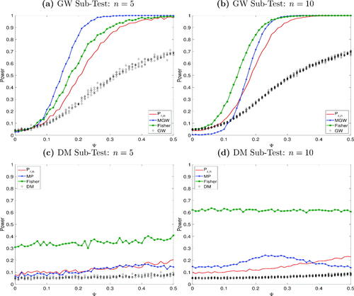
3.3.1 Low Dimensions

In the first Monte Carlo study, we simulate the loss differentials directly as a VAR(1) process to ensure both cross- and serial correlation:$$\Delta {\mathit{L}}_{t+1}=\mathit{\Psi }\Delta {\mathit{L}}_t+{\mathit{\epsilon }}_{t+1},\mathrm{\hspace{1em}}\mathrm{\hspace{1em}}\epsilon \sim \mathcal{N}(0,1),$$where $\Delta {\mathit{L}}_{t+1}=(\Delta L_{1,t+1},\dots ,\Delta L_{n,t+1})\prime$ and $t=1,\dots ,p$. The coefficients in the n × n matrix $\mathit{\Psi },{\psi }_{i,j}\in [{\psi }_l,{\psi }_u]$, are drawn randomly from a truncated standard normal distribution with upper and lower bounds ψ_u and ψ_l. We ensure the roots of $\mathit{\Psi }$ lie inside the unit circle by conditioning that its eigenvalues are smaller than one in absolute value. Additionally, to generate differences in test statistics, we impose $\mathit{\Psi }$ be lower triangular. The number of forecasts is set to $n=(5,10)$ with p = 200 periods each. The bounds are parameterized as ${\psi }_l=(0,-0.05,\dots ,-1)$ and ${\psi }_u=(0,0.05,\dots ,1)$. We then conduct GW and DM subtests for each of the n loss differentials. Notably, as soon as ${\psi }_l<0$ and ${\psi }_u>0$, the subhypothesis of all GW tests is no longer true. In contrast, the subhypothesis of the DM test, $\mathbb{E}[\Delta L_{i,t+1}]=0$, remains true on average. Based on the p-values of the individual tests, we compute the global test statistic $P_{r,n}$ and its power function. In addition, we conduct the multivariate GW test as well as the adjusted MP test jointly for all n loss differentials. For further comparison, we also report the Fisher statistic. The results are shown in Figure 1. The solid red line is the power function of the intersection union test. The black diamonds represent the power with which each subtest rejects its subhypothesis, the blue line corresponds to the multivariate GW and DM test, and the green line plots the Fisher test. We first consider the case of GW subtests. The power of our combined p-value statistic, is high regardless of n and higher than the power of individual GW tests. Its size also corresponds to the nominal level. The multivariate GW test performs well when n is small. However, it becomes increasingly undersized as n increases. Unreported simulations show that for n > 10, the covariance matrix of the multivariate GW test will be close to singular when $p\le 200$, meaning it is no longer consistent. The Fisher statistic exhibits slightly greater power than our test, and also greater power than the multivariate GW test for n = 10. Moving to the DM subtest, however, the Fisher statistic is extremely oversized. The MP and our test have roughly equal size for n = 5, but the former shows greater size distortions for n = 10. This simulation illustrates that, overall, our test has the best performance in a small dimensional scenario, regardless of the test type.

Fig. 1 Power functions IU test low dimensions. The figure reports the conditional predictive ability test of Giacomini and White (2006), GW, the multivariate GW test, MGW, the Diebold and Mariano (1995) test, DM, the Mariano and Preve (2012) test, MP, and the Fisher (1934) test. The x-axis reports the absolute values of the boundaries imposed on the distribution of $\mathit{\Psi }$.

3.3.2 Rejection Accuracy

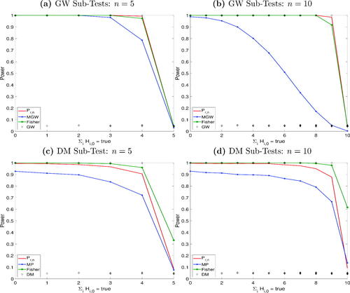
The second scenario we consider is one where $I=(0,1,\dots ,n)$ subhypotheses ${\mathcal{H}}_{i,0}$ are true, while n – I subhypotheses are false. More precisely, we increase the number of true subhypotheses from 0 to n and are interested in the question how accurately our test rejects in each case and in comparison to the multivariate GW test and the MP test. We use the same benchmarks as in the previous section. Specifically, we simulate$$\begin{array}{ccc}\Delta L_{i,t+1}\hfill & ={\epsilon }_{t+1},\hfill & \mathrm{}\text{for}\hspace{1em}i=0,\dots ,I,\hfill \\ \Delta L_{j,t+1}\hfill & =F_{t+1}+\psi \Delta L_{j,t}+{\nu }_{t+1},\mathrm{\hspace{1em}}\mathrm{\hspace{1em}}\hfill & \mathrm{}\text{for}\hspace{1em}j=I+1,\dots ,n,\hfill \\ F_{t+1}\hfill & =\mu +\psi F_t+{\eta }_{t+1}.\hfill & \hfill \end{array}$$

Here, ${\epsilon }_t,{\nu }_t,{\eta }_t\sim \mathcal{N}(0,1)$. The coefficient ψ is fixed at 0.3 and μ is set to be 0.5. We ran unreported simulations with different values for the coefficients which did not change the overall picture of the results. F_t, the common factor across loss differentials, is the source of dependence. We set $n=(5,10)$, noting that the ratio of n and p will impact the power of the multivariate GW and MP tests. The results are reported in Figure 2. The top panel shows the power functions based on GW subtests. Our test has consistently greater power than the multivariate GW test as well as the Fisher test. Indeed, for n = 10, the rejection pattern of the multivariate GW test looks remarkably different. The bottom two figures consider DM subtests. The MP test has lower power than our test and appears oversized when all null hypotheses are true for n = 10. Its power curve has steepened slightly, albeit less than the multivariate GW test. Although the Fisher test has slightly higher power than our test, it has a high likelihood of incorrectly rejecting the global null hypothesis when it is, in fact, true. Overall, the IU test exhibits the highest rejection accuracy. This simulation highlights that it is not obvious when the multivariate DM and GW tests reject their null hypotheses, obscuring the interpretability of their results.

Fig. 2 Power functions IU test rejection accuracy. The figure reports the conditional predictive ability test of Giacomini and White (2006), GW, the multivariate GW test, MGW, the Diebold and Mariano (1995) test, DM, the Mariano and Preve (2012) test, MP, and the Fisher (1934) test. The x-axis reports the absolute number of the true null hypotheses.

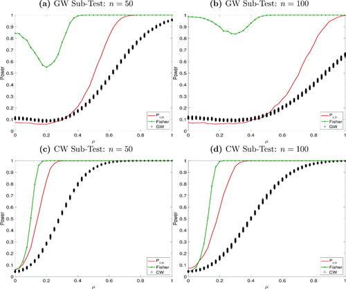
3.3.3 High Dimensions

In the third scenario, we consider a large n × T framework and generate artificial rolling-window one-step-ahead forecasts instead of simulating the loss differential directly. we simulating nested models and therefore report results for GW and the CW subtests. Define the estimation window as h and the out-of-sample window as p such that $T=h+p+1$ equals the total number of observations. First, we generate a random matrix U whose elements are uniform on $[-0.5,0.5]$ which can easily be transformed into a symmetric positive definite matrix $\mathit{\Sigma }=\mathit{UU}\prime$. This, in turn, can be used to generate a random $n\times T$ matrix with dependent rows, ${\mathit{Z}}_i=\mathcal{N}(0,\mathit{\Sigma })$, such that $\mathit{Z}=({\mathit{Z}}_1,{\mathit{Z}}_2,\dots ,{\mathit{Z}}_n$), where ${\mathit{Z}}_i$ are $T\times 1$. The Z matrices are used to generate $n\times 1$ vectors ${\mathit{X}}_t=\varphi {\mathit{X}}_{t-1}+{\mathit{Z}}_t$, with $\varphi =0.3$. We summarize the information in X in form of a common factor using the principal components estimator laid out in Bai (2003) and specify the process ${\mathit{Y}}_{\mathit{t}}=\mathit{\mu }+{\mathit{X}}_t$, for $t=1,\dots ,T,$ and generate two different forecasts for each of the n variables in ${\mathit{Y}}_t$:$$\begin{array}{cc}{\widehat{Y}}_{i,t+1}^{(1)}\hfill & =\widehat{\mu }+{\widehat{\beta }}_{1,i}{\tilde{F}}_{1,t+1},\hfill \\ {\widehat{Y}}_{i,t+1}^{(2)}\hfill & ={\widehat{\beta }}_{2,i}{\tilde{F}}_{1,t+1},\hfill \end{array}$$for $i=1,\dots ,n$. The coefficients are estimated using OLS over a rolling window of size h. The total number of forecasts for each model is p. ${\tilde{F}}_{1,t}$ is the first principal component estimate of X and for simplicity its value in t + 1 is assumed known. The forecast loss is specified to be quadratic, that is, $L_{i,t+1}^{(1)}={(Y_{i,t+1}-{\widehat{Y}}_{i,t+1}^{(1)})}^2$. We parameterize $\mathit{\mu }$ such that each ${\mu }_i=(0,0.1,\dots ,1)$. That is, for ${\mu }_i=0$, the subhypothesis is true for both GW and the CW subtest. The number of variables is set to $n=(50,100)$, the estimation window to h = 100 and p = 200 such that T = 301. In a large n framework, the consistent computation of the multivariate GW and MP tests is no longer feasible. Therefore, we only present the results of the Fisher test. The power functions are depicted in Figure 3. Considering first the GW subtests, the top figures bear out the fact that Fisher’s statistic exhibits considerable size distortions—exemplifying the need for appropriate corrections when considering dependent p-values. On the other hand, the IU test has low power for smaller values of μ, in line with the individual GW tests. As μ increases, however, the power of our test surpasses that of GW subtests. In contrast, for the CW test, it is slightly oversized and the divergence relative to the power of the individual tests is even more visible. Fisher’s method displays moderately greater power.

Fig. 3 Power functions IU test high dimensions. The figure reports the conditional predictive ability test of Giacomini and White (2006), GW the Clark and West (2007) test, CW, and the Fisher (1934) test. The x-axis reports the mean of the first DGP.

The simulations highlight that the IU test we propose in this article is a very reliable test for forecast accuracy in the presence of dependence. Whilst other tests may have higher power in some scenarios, they exhibit large Type I errors in others. We are able to confirm that our test most accurately rejects (sustains) the false (true) global null hypothesis of equal predictive ability across forecasts. The simulations substantiate that the intersection union test has good size and power properties regardless of dependence structures or dimensions.

4 Empirical Illustration

This section provides an empirical illustration of the test. As interdependencies are ubiquitous in financial data, exchange rate forecasts are well suited to apply our test. If a currency appreciates against the U.S.-Dollar (USD) following the release of positive macroeconomic data, we would expect to see similar movements in its exchange rate against, say, the Euro (EUR). Dependencies are also reflected in common factors that explain currency variations, for example carry, momentum, or value factors. As such factors affect multiple currencies simultaneously, one can expect a model that is able to predict these elements for one FX rate to have an elevated likelihood of predicting them for others. Likewise, if a test only indicates predictive ability in a single instance out of many, this may well be a false positive (Harvey, Liu, and Zhu 2016). Altogether, this strengthens the argument that one cannot disregard dependencies in the evaluation of exchange rate forecasts.

We compile a large daily dataset of 84 exchange rates, consisting of 39 currencies vis-a-vis the USD, 23 currencies against the EUR, and 22 currencies against the British Pound (GBP). The three exchange rates USD-GBP, USD-EUR, and GBP-EUR are only included once. USD currency pairs are obtained from the Bank for International Settlements (BIS), EUR currency pairs from the European Central Bank (ECB), and GBP currency pairs from the Bank of England (BoE). The dataset spans from January 4, 2011 to April 1, 2021, a total number of 2558 observations for the USD, 2590 for the GBP, and 2622 for the EUR. We use the dataset to generate out-of-sample forecasts for each exchange rate and compare the performance of different models across currencies and tests. The aim is to show the main characteristics of the test in a scenario where some, but not all, individual tests reject for some models. Thereby, we illustrate how our test addresses mixed evidence problems. Moreover, we demonstrate how the test can be applied to different combinations of exchange rates, models, and individual tests. To this end, we estimate three models for each of the 84 exchange rates in our sample, a constant coefficients (CC) AR(1) model, and AR(2) model as well as a time-varying parameter (TVP) AR(1) model, estimated via maximum likelihood:$$\begin{array}{cc}\Delta e_{i,t}\hfill & ={\beta }_{i,1}\Delta e_{i,t-1}+{\nu }_{i,t},\hfill \\ \Delta e_{i,t}\hfill & ={\beta }_{i,2}\Delta e_{i,t-1}+{\beta }_{i,3}\Delta e_{i,t-2}+{\eta }_{i,t},\hfill \\ \Delta e_{i,t}\hfill & ={\gamma }_{i,t}\Delta e_{i,t-1}+{\epsilon }_{i,t},\hfill \\ {\gamma }_{i,t}\hfill & ={\rho }_i{\gamma }_{i,t-1}+{ϵ}_{i,t}.\hfill \end{array}$$

Here, $i=1,2,\dots ,84$ and $\Delta e_{i,t}$ is the first difference of the log-FX rate. For each model, we generate one-step-ahead rolling window forecasts with an estimation window R of 750 for all exchange rates. We rely on the simulations of CW that show their MSPE-adjusted statistic performs well if p/R converges to a finite constant. The GW test requires $p\to \infty$ while R remains fixed. However, their simulations show the test statistic exhibits excellent properties for the p/R ratios used here. This yields a total of 3 × 84 forecasts. We compare both the TVP-AR(1) and CC-AR(2) forecasts with the CC-AR(1) forecasts using GW, CW, and DM subtest. The latter is not designed for nested models (Diebold 2015); however, as it remains one of the most widely used tests, we include it nonetheless for illustrative purposes, emphasizing that its results should be taken with a grain of salt. For both GW and DM subtest we use the loss differentials $\Delta L_{i,t+1}^{(1)}=\{L_{i,t+1}^{\text{AR}(1)}-L_{i,t+1}^{\text{AR}(2)}\}$ and $\Delta L_{i,t+1}^{(2)}=\{L_{i,t+1}^{\text{AR}(1)}-L_{i,t+1}^{\text{TVP}}\}$, where $L_{i,t+1}^{(m)}$ is the quadratic loss function of model m. This results in three different forecast accuracy tests being applied to compare the predictive ability of two models relative to a CC-AR(1) process for 84 exchange rates (USD + EUR + GBP), that is, $3\times 2\times 84=504$ test statistics and p-values, respectively. Table 2 fleshes out the absolute number of rejections of each subhypothesis at the 5%-level per model and currency. In addition, the table reports the number of rejections relative to the total number of tests conducted in each category. For instance, the GW subtest rejects the null hypothesis that the CC-AR(2) and CC-AR(1) model display equal predictive ability twice for USD currency pairs. We have performed this test for each USD exchange rate in the dataset, that is, 39 times, and only rejected in 5.1% of all cases. In several cases, the rejection rate is below 5%, that is, in a range one would expect given a false discovery rate equal to the nominal size of the tests. The null hypothesis of equal predictive accuracy between TVP-AR(1) and CC-AR(1) is rejected more frequently, especially by the CW subtest.

Table 2 Rejections for each individual test.

	USD				EUR				GBP
	AR(2)	(%)	TVP	(%)	AR(2)	(%)	TVP	(%)	AR(2)	(%)	TVP	(%)
CW	1	2.6	16	41.0	0	0	5	21.7	1	4.5	6	27.3
DM	1	2.6	3	7.7	4	17.4	1	4.3	6	27.3	1	4.5
GW	2	5.1	4	10.3	0	0	1	4.3	4	18.2	0	0

NOTE: The table contains the total number of rejections for each test as well as the number of rejections in percent of the total number of forecasts. AR(2) refers to CC-AR(2) compared to CC-AR(1) forecasts, while TVP refers to TVP-AR(1) forecasts compared to CC-AR(1) forecasts.

We proceed by demonstrating that combining the individual p-values through our test is a convenient way to compute a global test statistic both when looking at USD, EUR, or GBP in isolation (small n) and for combinations of the three currencies or tests (large n). Panel A in Table 3 reports the test statistic of the IU test for USD, EUR, and GBP. The first three rows display the IU test statistic combining the p-values from each of the sub-tests: GW, CW, and DM. The first two columns CC-AR(2) and TVP-AR(1) contain the results combining the p-values of each subtest, comparing the CC-AR(2) and TVP-AR(1) forecasts, respectively, with the CC-AR(1) forecasts for exchange rates against the USD. The statistics in these columns indicate whether there is evidence against the global null hypothesis of equal predictive ability between the two forecasts and a CC-AR(1) across all exchange rates in the sample that are quoted against the USD. The third column, Combined (Comb.), combines the p-values of the two preceding columns. The global null hypothesis is now that there is equal predictive ability between either of the two forecasts and a CC-AR(1), put differently, no available model produced better or worse forecasts than an CC-AR(1). In the fifth row, the p-values of the three subtests are combined together to ascertain whether there is evidence for predictive accuracy across different test types. The results for exchange rates quoted against EUR and GBP are reported analogously in the subsequent columns. It is common to use different individual tests to assess forecasting performance, hence, we view this as an important application for our methodology, as the subtests may yield conflicting results. Our methodology allows researchers to formulate and evaluate a global null hypothesis of equal predictive accuracy across different types of subtests.

Table 3 Test statistic for combined p-values.

Panel A: Individual currencies
	USD			EUR			GBP
	AR(2)	TVP	Comb.	AR(2)	TVP	Comb.	AR(2)	TVP	Comb.
CW	0.9	17.9*	8.9	0.1	12.2*	6.1	2.6	26.9**	13.4*
DM	0.9	2923.2***	1461.6***	4.3	1.3	2.2	6.9	1.5	3.4
GW	4.7	374.2***	187.1***	0.7	2.3	1.1	2.3	0.3	1.1
n	39	39	78	23	23	46	22	22	44
All	1.6	974.4***	487.2***	1.4	4.1	2.0	2.3	9.0	4.5
n	117	117	234	69	69	138	66	66	132
Panel B: Combined currencies
	USD-EUR			USD-GBP			EUR-GBP			All
	AR(2)	TVP	Comb.	AR(2)	TVP	Comb.	AR(2)	TVP	Comb.	AR(1)	TVP	Comb.
CW	1.0	11.4*	5.7	0.5	11.2*	5.6	1.3	13.1*	6.6	0.7	8.3	4.2
DM	2.5	1869.0***	934.5***	1.6	1838.8***	919.4***	3.4	0.8	1.7	1.8	1357.2***	678.6***
GW	3.0	239.3***	119.6***	2.9	235.4***	117.7***	1.1	1.2	0.6	2.2	173.7***	86.9**
n	62	62	124	61	61	122	45	45	90	84	84	168
All	1.0	612.9***	306.5***	1.0	623.0***	311.5***	1.1	4.4	2.2	0.7	452.4***	226.2***
n	186	186	372	183	183	366	135	135	270	252	252	504

NOTE: AR(2) refers to CC-AR(2) compared to CC-AR(1) forecasts, while TVP refers to TVP-AR(1) forecasts compared to CC-AR(1) forecasts. Panel A contains results from IU test for. GW stands for Giacomini-White test, CW for Clark-West test, and DM for Diebold-Mariano test. First two columns and first three rows contain test statistic of combined p-values from each tests for USD for each model. Third column contains test statistic for both models. Forth row contains test statistic for combined p-values from all tests for each model and for both models. Panel B contain test statistic for combined p-values from currency combinations for each test for each model and for both models as well as p-values from all tests combined for each model and for both models. Test rejects if statistic exceeds the critical values, obtained as $r/(\alpha (r-1))$: $\alpha =1\%$: 105.263, denoted by ${}^{***}$, $\alpha =5\%$: 21.053, denoted by ${}^{**},\alpha =10\%$: 10.526, denoted by ${}^{*}$.

Panel A presents scenarios with small to medium n which are reported in the respective rows. Stars indicate the significance level at which the test rejects. Starting with USD exchange rates, the global null hypothesis that the CC-AR(2) and the CC-AR(1) forecasts exhibit equal predictive ability across exchange rates is sustained for all test types for all three currencies. In contrast, the same global null hypothesis for the TVP-AR(1) forecasts is rejected when combining the individual p-values of both GW and DM tests (the CW test only rejects at the 10% level). When combining the p-values from all three tests, the global null hypothesis of equal predictive ability across exchange rates against the USD is also rejected. Likewise, the global null that neither model under- or outperforms a CC-AR(1) is rejected using the p-values of GW and DM tests as a basis as well as for all three tests combined. On the contrary, the same global null hypotheses can only be rejected at the 10%-level for CW tests considering GBP exchange rates. Barring a 5%-level rejection of the CW test for the TVP-AR(1) model in case of the GBP, and a 10%-level rejection for the EUR, no other global null is rejected. Suppose one faces the decision whether to use the TVP model or not. The findings give rise to the question whether evidence against equal predictive ability exists only for the USD or also for combinations of the three currencies. Our test can analyze the null hypothesis of equal predictive ability across such combinations, and thereby provide an indication on whether a model can be deemed suitable for USD modeling or also in more general scenarios. Panel B presents the results for currency combinations, with n taking medium to large values. The first three columns combine the p-values of USD and EUR with the three corresponding subcolumns defined as in Panel A. That is, the values in the first column reflect the global null that there is equal predictive ability between CC-AR(2) and CC-AR(1) across exchange rates vis-a-vis USD and EUR. The second column, which reports the results for an analogous null hypothesis for the TVP-AR(1), shows that the latter is rejected at the 1% level according to both GW and DM tests (and the CW test at the 10% level) as well as for all three tests combined. The same holds true for the global null that no model under- or outperforms a CC-AR(1) for USD and EUR combined. The results are identical for USD and GBP combined. On the contrary, there is no evidence that any or both models perform differently than a CC-AR(1) when only considering p-values of EUR and GBP. The results should be interpreted bearing in mind that there are several rejections by the underlying individual tests, as reported in Table 2. However, this does not translate into an automatic rejection of the global null hypothesis, as the IU test accounts for dependence and false discovery. Finally, in the last column, we combine the p-values of all three currencies. The global null of equal predictive ability of TVP- and CC-AR(1) across USD, EUR, and GBP is rejected when combining the p-values of GW and DM tests. The global null that no forecast is better or worse than a CC-AR(1) forecast is rejected for both GW and DM tests at the 1% and 5% level. Next, we combine the p-values of all three tests, leading to the global null hypothesis that there is equal predictive ability across all currencies regardless of the underlying test. When tested for the TVP forecasts (penultimate column, fifth row) and for all forecasts (final column, fifth row), the global null is rejected at the 1% level. That is, there is evidence that, across all currencies, and all tests the TVP-AR(1) forecasts differ significantly from the CC-AR(1) forecasts. What is more, there is evidence that across currencies, and tests, forecasts of either model differ significantly from CC-AR(1) forecasts. To summarize, the set of univariate tests conducted presents mixed evidence with generally few rejections. Through our IU test, we are able to formulate a range of global null hypotheses, based on different combinations of univariate tests. Thereby, we can present statistically significant evidence that a time-varying AR(1) model is able to produce superior forecasts compared to a constant coefficients model for currencies quoted against the USD. These results continue to hold when considering USD together with EUR or GBP exchange rates.

5 Conclusions

In this article, we proposed an intersection-union multivariate forecasting accuracy test. The test is constructed using p-values of existing univariate tests that are treated as subtests and combined to evaluate a global null hypothesis of equal predictive ability across forecasts. Our test does not require any assumptions on the dependence structure between tests, and has a clearly defined rejection set. This is an important feature, as independence rarely holds in most forecasting exercises, and assuming independence may lead to considerable size distortions. In contrast, we proved that our test is level-α and consistent under the alternative. An extensive Monte Carlo simulation showed very good size properties of our test compared to conventional procedures of combining p-values, by conducting the intersection-union test using three popular univariate subtests of predictive ability. We showed that the properties of our multivariate procedure are unaffected by the number of subtests. To examine the power of the test, we simulated three different forecasting scenarios: a low dimensional scenario with changing cross-dependence, one that illustrated the rejection accuracy of our test, and, finally, a high-dimensional scenario. Our test showed high power in all cases. We compared our test to alternative benchmark procedures, each of which exhibited considerable limitations. An empirical illustration underpinned the wide applicability of our test. We compiled a large dataset of 84 daily exchange rates, quoted against USD, GBP, and EUR, to examine whether a time-varying AR(1) or a constant coefficients AR(2) model delivered different forecasts with respect to a constant coefficients AR(1) model. We also analyzed this across various combinations of currency pairs. While the results of the subtests themselves were mixed, our intersection-union test provided statistically significant evidence that the time-varying parameter model outperformed both of the constant coefficient models across combinations of currencies.

Acknowledgments

We thank the Editor, Christian Hansen, an Associate Editor, and two anonymous Referees whose useful comments and suggestions greatly helped to improve the content and the presentation of the article. We also thank Giuliano de Rossi, Kate Phylaktis, and Roy Batchelor for insightful comments and discussions. Special acknowledgments to Lynda Khalaf and Fa Wang for invaluable suggestions on a previous version of the article. The usual disclaimer applies.

Supplementary Materials

The supplementary materials include the proofs of the theoretical results, further descriptions regarding the multivariate application of the Giacomini and White (2006) test, additional stimulations on the choice of r, and the code to replicate the Monte-Carlo Simulations and Empirical Results in this article.

References

- Bai, J. (2003), “Inferential Theory for Factor Models of Large Dimensions,” Econometrica, 71, 135–171. DOI: 10.1111/1468-0262.00392.
- Carriero, A., Galvão, A. B., and Kapetanios, G. (2019), “A Comprehensive Evaluation of Macroeconomic Forecasting Methods,” International Journal of Forecasting, 35, 1226–1239. DOI: 10.1016/j.ijforecast.2019.02.007.
- Clark, T., and McCracken, M. (2013), “Advances in Forecast Evaluation,” in Handbook of Economic Forecasting (Vol. 2), eds. G. Elliot and A. Timmermann, pp. 1107–1201, Amsterdam: Elsevier.
- Clark, T. E., and West, K. D. (2007), “Approximately Normal Tests for Equal Predictive Accuracy in Nested Models,” Journal of Econometrics, 138, 291–311. DOI: 10.1016/j.jeconom.2006.05.023.
- Diebold, F. X. (2015), “Comparing Predictive Accuracy, Twenty Years Later: A Personal Perspective on the Use and Abuse of Diebold–Mariano Tests,” Journal of Business & Economic Statistics, 33, 1–9.
- Diebold, F. X., and Mariano, R. S. (1995), Comparing Predictive Accuracy,” Journal of Business & Economic Statistics, 13, 253–265.
- Donoho, D., and Jin, J. (2004), “Higher Criticism for Detecting Sparse Heterogeneous Mixtures,” The Annals of Statistics, 32, 962–994. DOI: 10.1214/009053604000000265.
- Fisher, R. A. (1934), Statistical Methods for Research Workers (Vol. 5), Edinburgh: Oliver and Boyd.
- Giacomini, R., and White, H. (2006), “Tests of Conditional Predictive Ability,” Econometrica, 74, 1545–1578. DOI: 10.1111/j.1468-0262.2006.00718.x.
- Harvey, C. R., Liu, Y., and Zhu, H. (2016), “… and the Cross-section of Expected Returns,” The Review of Financial Studies, 29, 5–68. DOI: 10.1093/rfs/hhv059.
- Heard, N. A., and Rubin-Delanchy, P. (2018), Choosing Between Methods of Combining p-values,” Biometrika, 105, 239–246. DOI: 10.1093/biomet/asx076.
- Kost, J. T., and McDermott, M. P. (2002), “Combining Dependent p-values,” Statistics and Probability Letters, 60, 183–190. DOI: 10.1016/S0167-7152(02)00310-3.
- Laurent, S., Rombouts, J. V., and Violante, F. (2013), “On Loss Functions and Ranking Forecasting Performances of Multivariate Volatility Models,” Journal of Econometrics, 173, 1–10. DOI: 10.1016/j.jeconom.2012.08.004.
- Liu, Y., and Xie, J. (2019), Accurate and Efficient p-value Calculation via Gaussian Approximation: A Novel Monte-Carlo Method,” Journal of the American Statistical Association, 114, 384–392. DOI: 10.1080/01621459.2017.1407776.
- Liu, Y., and Xie, J. (2020), “Cauchy Combination Test: A Powerful Test with Analytic p-value Calculation Under Arbitrary Dependency Structures,” Journal of the American Statistical Association, 115, 393–402. DOI: 10.1080/01621459.2018.1554485.
- Mariano, R. S., and Preve, D. (2012), Statistical Tests for Multiple Forecast Comparison,” Journal of Econometrics, 169, 123–130. DOI: 10.1016/j.jeconom.2012.01.014.
- Qu, R., Timmermann, A., and Zhu, Y. (in press), “Comparing Forecasting Performance in Cross-sections,” Journal of Econometrics.
- Robins, J. M., van der Vaart, A., and Ventura, V. (2000), “Asymptotic Distribution of p-values in Composite Null Models,” Journal of the American Statistical Association, 95, 1143–1156.
- Van der Vaart, A. W. (2000), Asymptotic Statistics (Vol. 3), Cambridge: Cambridge University Press.
- Vovk, V., and Wang, R. (2020), “Combining p-values via Averaging,” Biometrika, 107, 791–808. DOI: 10.1093/biomet/asaa027.