Detection of Multiple Structural Breaks in Large Covariance Matrices

ABSTRACT

This article studies multiple structural breaks in large contemporaneous covariance matrices of high-dimensional time series satisfying an approximate factor model. The breaks in the second-order moment structure of the common components are due to sudden changes in either factor loadings or covariance of latent factors, requiring appropriate transformation of the factor models to facilitate estimation of the (transformed) common factors and factor loadings via the classical principal component analysis. With the estimated factors and idiosyncratic errors, an easy-to-implement CUSUM-based detection technique is introduced to consistently estimate the location and number of breaks and correctly identify whether they originate in the common or idiosyncratic error components. The algorithms of Wild Binary Segmentation for Covariance (WBS-Cov) and Wild Sparsified Binary Segmentation for Covariance (WSBS-Cov) are used to estimate breaks in the common and idiosyncratic error components, respectively. Under some technical conditions, the asymptotic properties of the proposed methodology are derived with near-optimal rates (up to a logarithmic factor) achieved for the estimated breaks. Monte Carlo simulation studies are conducted to examine the finite-sample performance of the developed method and its comparison with other existing approaches. We finally apply our method to study the contemporaneous covariance structure of daily returns of S&P 500 constituents and identify a few breaks including those occurring during the 2007–2008 financial crisis and the recent coronavirus (COVID-19) outbreak. An $\mathrm{R}$ package “$\mathrm{BSCOV}$” is provided to implement the proposed algorithms.

KEYWORDS:

• Approximate factor models
• Binary segmentation
• CUSUM
• Large covariance matrix
• Principal component analysis
• Structural breaks

1 Introduction

Estimation of covariance matrices is of fundamental importance in modern multivariate statistics, and has applications in various fields such as biology, economics, finance, and social networks. Suppose that $\left({\mathit{X}}_t:t=1,\dots ,n\right)$ is a collection of n observations from a d-dimensional random vector with $\mathrm{E}({\mathit{X}}_t)=\mathbf{0}$ and $\mathrm{E}\left({\mathit{X}}_t{\mathit{X}}_t^{\mathrm{⊺}}\right)=\mathbf{\Sigma }$, where $\mathbf{0}$ is a null vector whose size may change from line to line and $\mathbf{\Sigma }$ is a d × d positive definite covariance matrix. When the dimension d is fixed or significantly smaller than the sample size n, the population covariance matrix $\mathbf{\Sigma }$ can be well estimated by the conventional sample covariance matrix (see Anderson 2003):(1.1) $${\overline{\mathbf{\Sigma }}}_n=\frac{1}{n}\sum _{t=1}^n\left({\mathit{X}}_t-{\overline{\mathit{X}}}_n\right){\left({\mathit{X}}_t-{\overline{\mathit{X}}}_n\right)}^{\mathrm{⊺}},\hspace{1em}{\overline{\mathit{X}}}_n=\frac{1}{n}\sum _{t=1}^n{\mathit{X}}_t.$$(1.1)

However, when d exceeds n, the sample covariance matrix ${\overline{\mathbf{\Sigma }}}_n$ defined in (1.1) becomes singular. Estimation of such a large covariance matrix is generally challenging and has received increasing attention in recent years. Some techniques have been introduced to regularize covariance matrices and produce reliable estimation (see Wu and Pourahmadi 2003; Ledoit and Wolf 2004; Bickel and Levina 2008a, 2008b; El Karoui 2008a, 2008b; Lam and Fan 2009; Rothman, Levina, and Zhu 2009; Cai and Liu 2011; Fan, Liao, and Mincheva 2013; Huang and Fryzlewicz 2019). A comprehensive review on large covariance matrix estimation can be found in Pourahmadi (2013), Cai, Ren, and Zhou (2016) and Fan, Liao, and Liu (2016). All of the aforementioned literature assumes that the large covariance matrix is a constant matrix throughout the entire course of data collection, which may be too restrictive in practical situations. Some recent papers including Chen, Xu, and Wu (2013) and Chen and Leng (2016) attempt to relax this restriction and consider a large dynamic covariance matrix estimation by allowing the covariance matrix to evolve smoothly over time (or with an index variable).

The main interest of this article is to detect and estimate multiple structural breaks in large covariance matrices, to which setting the methodology in Chen, Xu, and Wu (2013) and Chen and Leng (2016) is no longer applicable. Structural breaks are very common in many areas such as economics and finance, and may occur for various reasons. If such abrupt structural changes are ignored in covariance matrix estimation, subsequent statistical analysis would lead to invalid inference and misleading conclusions. The classical Binary Segmentation (BS) technique is commonly used to detect structural breaks, and has been extensively studied since its introduction by Vostrikova (1981). For instance, in the setting of univariate mean regression models, theoretical properties, computational algorithms and relevant empirical applications of the traditional BS and its generalized version have been systematically studied by Venkatraman (1992), Bai (1997), Cho and Fryzlewicz (2012), Killick, Fearnhead, and Eckley (2012), Fryzlewicz (2014, 2020) and the references therein. In recent years, there has been increasing interest in extending this technique to high-dimensional settings such as high-dimensional time series and large panel data (see Cho and Fryzlewicz 2015; Jirak 2015; Cho 2016; Aston and Kirch 2018; Wang and Samworth 2018; Wang et al. 2019; Safikhani and Shojaie 2022). However, most of the aforementioned literature mainly considers break detection and estimation in the first-order moment structure. Aue et al. (2009) use the BS method with mean-corrected cumulative sum (CUSUM) to detect structural breaks in fixed dimensional covariance matrices, and establish the limit distributions for the test statistics and the convergence rate for the estimated break date. Korkas and Fryzlewicz (2017) detect breaks in the second-order moment structure of time series by combining the wavelet-based transformation and the univariate Wild Binary Segmentation (WBS) algorithm proposed by Fryzlewicz (2014). However, their technique is not directly applicable to our case when the size of the covariance matrix diverges to infinity as the sample size n increases.

In this article, we consider the second-order moment structure of the high-dimensional random vector ${\mathit{X}}_t$ generated by an approximate factor model, that is,(1.2) $${\mathit{X}}_t=\mathbf{\Lambda }{\mathit{F}}_t+{\mathit{ϵ}}_t,t=1,2,\dots ,n,$$(1.2) where $\mathbf{\Lambda }={({\lambda }_1,\dots ,{\lambda }_d)}^{\mathrm{⊺}}$ is a matrix of factor loadings with λ_i being an r-dimensional vector, ${\mathit{F}}_t$ is an r-dimensional vector of common factors, and ${\mathit{ϵ}}_t={({\mathrm{ϵ}}_{t1},\dots ,{\mathrm{ϵ}}_{td})}^{\mathrm{⊺}}$ is a d-dimensional vector of idiosyncratic components uncorrelated with ${\mathit{F}}_t$. The approximate factor model is very popular in economics and finance, and has become an effective tool in analyzing high-dimensional time series (see Chamberlain and Rothschild 1983; Fama and French 1992; Stock and Watson 2002; Bai and Ng 2002, 2006; Chen et al. 2018). Our main focus is the contemporaneous second-order moment structure, which plays a crucial role in various fields such as the classic mean-variance portfolio choice theory and risk management. Note that(1.3) $$\mathbf{\Sigma }=\text{cov}({\mathit{X}}_t)=\mathbf{\Lambda }\text{cov}({\mathit{F}}_t){\mathbf{\Lambda }}^{\mathrm{⊺}}+\text{cov}({\mathit{ϵ}}_t)=\mathbf{\Sigma }(\mathbf{\Lambda },\mathit{F})+\mathbf{\Sigma }(\mathit{ϵ}),$$(1.3) where $\mathbf{\Sigma }(\mathit{ϵ})$ is the covariance matrix of the idiosyncratic components ${\mathit{ϵ}}_t$ and $\mathbf{\Sigma }(\mathbf{\Lambda },\mathit{F})$ is the covariance matrix of the common components $\mathbf{\Lambda }{\mathit{F}}_t$. In this article, we aim to study multiple structural breaks in the covariance structure of ${\mathit{X}}_t$ generated by the approximate factor model, estimating the break points and number of breaks. Structural breaks may occur in either the covariance structure of the common components or that of the idiosyncratic components, indicating that the constant covariance structure in (1.3) is replaced by the following time-varying version:(1.4) $${\mathbf{\Sigma }}_t={\mathbf{\Sigma }}_t(\mathbf{\Lambda },\mathit{F})+{\mathbf{\Sigma }}_t(\mathit{ϵ}),t=1,\dots ,n.$$(1.4)

The main contributions of this article, the fundamental novelty of the proposed methodology and its connection to some recent literature are summarized as follows.

• A transformation mechanism is introduced to convert the approximate factor model with multiple structural breaks to that with constant factor loadings, justifying applicability of the classical Principal Component Analysis (PCA) technique (see Bai and Ng 2002; Stock and Watson 2002) to a more general model setting. Note that breaks in the second-order moment structure of the common components are due to changes in factor loadings, covariance of latent factors or factor number. This makes it challenging to directly estimate the latent common factors and factor loadings via PCA. When there are multiple breaks in factor loadings, we transform the original factor model to one with time-invariant factor loadings and a time-varying covariance structure for transformed factors, and then use the PCA method to estimate the transformed factors and factor loadings, which are shown to be consistent with convergence rates comparable to those in the existing literature on PCA for approximate factor models without breaks (see Bai and Ng 2002; Fan, Liao, and Mincheva 2013). This transformation technique is also used by Han and Inoue (2015) and Baltagi, Kao, and Wang (2017, 2021) to estimate and test factor models with structural instability. However, they assume that the number of factors does not change. In contrast, we consider a more general setting, allowing changes of factor numbers and multiple breaks in the covariance matrices of idiosyncratic components.

• With the estimated factors and idiosyncratic errors, we propose an easy-to-implement CUSUM-based detection technique to estimate the location and number of breaks and identify whether they originate in the common or idiosyncratic components. The developed CUSUM statistics are directly computed via the empirical second moments of the estimated factors and idiosyncratic errors. Based on Fryzlewicz’s (2014) WBS algorithm, we propose a Wild Binary Segmentation for Covariance (WBS-Cov) to locate multiple breaks in the common components. For breaks in the idiosyncratic error components, we introduce a Wild Sparsified Binary Segmentation algorithm for Covariance (WSBS-Cov), combining WBS-Cov and the Sparsified Binary Segmentation (SBS) proposed by Cho and Fryzlewicz (2015) in the high-dimensional mean estimation context. A recent paper by Barigozzi, Cho, and Fryzlewicz (2018) combines the wavelet-based transformation and the double CUSUM technique (Cho 2016) to estimate the break time as well as break number within the second-order moment structure. However, a disadvantage of the wavelet-based transformation on the piecewise-constant “signals,” involving selection of the wavelet filter and scale parameter, is that it could destroy the piecewise constancy and subsequently affect the estimation accuracy of the break number and location. When we only focus on a specific feature of the data, data transformation, even one-to-one transformation, would distort the interpretation of breaks of the structure. Another recent method to deal with sparsity in high-dimensional break detection is the sparse projection introduced by Wang and Samworth (2018) but their method only detects breaks in the first-order moment structure. Wang, Yu, and Rinaldo (2021) extends the BS and WBS techniques to detect multiple breaks in large covariance matrices, but they limit attention to the independent sub-Gaussian random vector and assume that the dimension is divergent at a slow polynomial rate of n. In contrast, we allow the dimension to grow faster, for example, at an exponential rate of n, a typical setting in big data analysis.

• Simulation studies are implemented to assess the finite-sample performance of the proposed method and its comparison with other competing methods. The simulation results show that our method has superior numerical performance in most settings, whereas the method by Barigozzi, Cho, and Fryzlewicz (2018) tends to perform poorly when the number of covariance matrix entries with breaks is small relative to the matrix size. Our simulation also shows that the proposed methods are robust when the factor number is over-estimated.

• The developed model and method are applied to the daily return series of S&P 500 constituent which contain 375 firms over the period from January 01, 2000 to February 28, 2021, and detect five breaks in the covariance structure of the common components and three breaks in the idiosyncratic error components. In particular, we identify the breaks occurring during the 2007–2008 global financial crisis and the recent coronavirus (COVID-19) outbreak. With an additional comparison with break detection result of low-dimensional observable risk factor series, we emphasize that the breaks in covariance structure of returns cannot be fully explained by the breaks in the covariance structure of observed risk factors nor the breaks in loadings of these factors.

The rest of the article is organized as follows. Section 2 introduces the setting of multiple structural breaks, the PCA estimation and CUSUM-based detection methods, and the WBS-Cov and WSBS-Cov algorithms. Section 3 presents the asymptotic theory for the developed WBS-Cov and WSBS-Cov methods. Section 4 discusses some practical issues in the detection procedure. Sections 5 and 6 give the simulation studies and the empirical application, respectively. Section 7 concludes the article. The technical assumptions are given in Appendix A and proofs of the main theoretical results are available in Appendices C–E of a supplementary materials. An $\mathrm{R}$ package “$\mathrm{BSCOV}$” for implementing the proposed methods is available from https://github.com/markov10000/BSCOV. Throughout the article, we let $\left|\right|·|{|}_2$ and $\left|\right|·|{|}_F$ denote the Euclidean norm of a column vector and the Frobenius norm of a matrix, respectively; let $\text{vech}(·)$ denote the half vectorization of a symmetric matrix obtained by vectorizing only the lower triangular part of the matrix; let $\lfloor ·\rfloor$ denote the floor function; let $a\vee b$ and $a\wedge b$ denote $\max \{a,b\}$ and $\min \{a,b\}$, respectively; and let $a_n\mathrm{\asymp }{b}_n$ denote that $a_n=O(b_n)$ and $b_n=O(a_n)$ hold jointly.

2 Methodology

In this section, we first introduce the setting of multiple structural breaks in the contemporaneous covariance structure of both the common and idiosyncratic components, and transform the approximate factor models to construct PCA estimation of the latent common factors and factor loadings (with appropriate rotation). Using the estimated factors and idiosyncratic errors, we then introduce the CUSUM-based statistics to estimate the location and number of structural breaks as well as the WBS-Cov and WSBS-Cov algorithms.

2.1 Model Structure for Multiple Structural Breaks

We consider the following multiple structural breaks in the covariance matrix of the common components, that is, ${\mathbf{\Sigma }}_t(\mathbf{\Lambda },\mathit{F})$ in (1.4) is specified as(2.1) $${\mathbf{\Sigma }}_t(\mathbf{\Lambda },\mathit{F})=\{\text{}\begin{array}{cc}{\mathbf{\Sigma }}_1^0(\mathbf{\Lambda },\mathit{F}),& 1\le t\le {\eta }_1^c,\\ {\mathbf{\Sigma }}_2^0(\mathbf{\Lambda },\mathit{F}),& {\eta }_1^c+1\le t\le {\eta }_2^c,\\ ⋮& ⋮\\ {\mathbf{\Sigma }}_{K_1+1}^0(\mathbf{\Lambda },\mathit{F}),& {\eta }_{K_1}^c+1\le t\le n,\end{array}$$(2.1) where ${\mathbf{\Sigma }}_k^0(\mathbf{\Lambda },\mathit{F})\ne {\mathbf{\Sigma }}_{k+1}^0(\mathbf{\Lambda },\mathit{F})$ for $k=1,\dots ,K_1$, and ${\eta }_1^c,\dots ,{\eta }_{K_1}^c$ are unobservable breaks with the superscript “c” denoting the “common component.” For convenience, we let ${\eta }_0^c=0$ and ${\eta }_{K_1+1}^c=n$. The above structural breaks may be caused by one or a combination of the following cases,

• Case (i): sudden changes in the factor loadings;

• Case (ii): sudden changes in the covariance matrix for common factors;

• Case (iii): sudden changes in the number of factors.

Let ${\mathbf{\Lambda }}_k^0$ be a $d\times r_k$ factor loading matrix and ${\mathit{F}}_{t,k}$ be the corresponding factor vector with dimension r_k when ${\eta }_{k-1}^c+1\le t\le {\eta }_k^c$, and write the approximate factor model as(2.2) $${\mathit{X}}_t={\mathbf{\Lambda }}_k^0{\mathit{F}}_{t,k}+{\mathit{ϵ}}_t,{\eta }_{k-1}^c+1\le t\le {\eta }_k^c.$$(2.2)

Letting ${\mathbf{\Sigma }}_k^0(\mathbf{\Lambda },\mathit{F})={\mathbf{\Lambda }}_k^0\text{cov}({\mathit{F}}_{t,k}){({\mathbf{\Lambda }}_k^0)}^{\mathrm{⊺}}$, the structural break structure (2.1) can be equivalently written as$${\mathbf{\Sigma }}_t(\mathbf{\Lambda },\mathit{F})=\{\mathrm{}\mathrm{}\begin{array}{cc}{\mathbf{\Lambda }}_1^0\text{cov}({\mathit{F}}_{t,1}){({\mathbf{\Lambda }}_1^0)}^{\mathrm{⊺}},& 1\le t\le {\eta }_1^c,\\ {\mathbf{\Lambda }}_2^0\text{cov}({\mathit{F}}_{t,2}){({\mathbf{\Lambda }}_2^0)}^{\mathrm{⊺}},& {\eta }_1^c+1\le t\le {\eta }_2^c,\\ ⋮& ⋮\\ {\mathbf{\Lambda }}_{K_1+1}^0\text{cov}({\mathit{F}}_{t,K_1+1}){({\mathbf{\Lambda }}_{K_1+1}^0)}^{\mathrm{⊺}},& {\eta }_{K_1}^c+1\le t\le n.\end{array}$$

Note that, although ${\mathbf{\Sigma }}_k^0(\mathbf{\Lambda },\mathit{F})\ne {\mathbf{\Sigma }}_{k+1}^0(\mathbf{\Lambda },\mathit{F})$ for $k=1,\dots ,K_1,{\mathbf{\Lambda }}_k^0$ may be the same as ${\mathbf{\Lambda }}_{k+1}^0$ (when cases (i) and (iii) do not occur at the break time). It is worthwhile to point out that case (i) is similar to the approximate factor model with structural breaks; see, for example, Breitung and Eickmeier (2011), Chen, Dolado, and Gonzalo (2014), Han and Inoue (2015), Cheng, Liao, and Schorfheide (2016), Baltagi, Kao, and Wang (2017), Bai, Han, and Shi (2020), and Duan, Bai, and Han (2022). However, the aforementioned papers consider the case of a single structural break in the factor loadings and usually assume that the covariance of the idiosyncratic error components is time invariant. Ma and Su (2018) consider detecting and estimating multiple structural breaks in the factor loadings with a three-step procedure using the adaptive fused group Lasso. Case (iii) is an important type of structure break in the factor model, which has received much attention in recent years (see Baltagi, Kao, and Wang 2017; Barigozzi, Cho, and Fryzlewicz 2018; Li et al. 2019). Section 2.2 will give a unified factor model framework covering cases (i)–(iii) which facilitates the construction of PCA estimation, and then proceed to introduce the relevant CUSUM statistics in Section 2.3 to detect the multiple structural breaks in the common component.

The structural breaks in the covariance matrix of the error components are specified as follows$${\mathbf{\Sigma }}_t(\mathit{ϵ})=\{\begin{array}{cc}{\mathbf{\Sigma }}_1^0(\mathit{ϵ}),& 1\le t\le {\eta }_1^e,\\ {\mathbf{\Sigma }}_2^0(\mathit{ϵ}),& {\eta }_1^e+1\le t\le {\eta }_2^e,\\ ⋮& ⋮\\ {\mathbf{\Sigma }}_{K_2+1}^0(\mathit{ϵ}),& {\eta }_{K_2}^e+1\le t\le n,\end{array}$$and ${\mathbf{\Sigma }}_k^0(\mathit{ϵ})\ne {\mathbf{\Sigma }}_{k+1}^0(\mathit{ϵ})$ for $k=1,\dots ,K_2$, where ${\eta }_1^e,\dots ,{\eta }_{K_2}^e$ are unobservable breaks with the superscript “e” denoting the “idiosyncratic error component.” For convenience, we let ${\eta }_0^e=0$ and ${\eta }_{K_2+1}^e=n$.

Let(2.3) $${\mathcal{B}}^c=\left\{{\eta }_1^c,\dots ,{\eta }_{K_1}^c\right\}\text{and}{\mathcal{B}}^e=\left\{{\eta }_1^e,\dots ,{\eta }_{K_2}^e\right\}.$$(2.3)

In this article, we assume that the minimum length of the subintervals separated by ${\eta }_k^c$ is of order n, see Assumption 4(ii) in Appendix A. Such a restriction is mainly to ensure that the PCA method is applicable to estimate the latent factors and factor loadings. In contrast, the minimum length of the subintervals separated by ${\eta }_k^e$ is allowed to be of order smaller than n, see Assumption 4(iii). We do not impose any restriction on how the break points in ${\mathcal{B}}^c$ and those in ${\mathcal{B}}^e$ are located with respect to each other.

2.2 Transformed Factor Models and PCA Estimation

Although the multiple structural breaks formulated in (2.1) and (2.2) may be caused by one or a combination of cases (i)–(iii) described in Section 2.1, we next show that multiple structural breaks in the factor loadings and factor number can be transformed to breaks in the factor covariance structure.

Proposition 2.1.

The approximate factor model (2.2) can be equivalently written as a transformed factor model like(2.4) $${\mathit{X}}_t={\mathbf{\Lambda }}^{\mathrm{\star }}{\mathit{F}}_t^{\mathrm{\star }}+{\mathit{ϵ}}_t,t=1,\dots ,n,$$(2.4) where ${\mathbf{\Lambda }}^{\mathrm{\star }}$ denotes the transformed factor loading matrix which is time invariant, and ${\mathit{F}}_t^{\mathrm{\star }}$ denotes the transformed factors. In addition, the number of factors in the original factor model and that in the transformed factor model, satisfy the following inequalities,(2.5) $$\underset{1\le k\le K_1+1}{\max }{\underset{¯}{r}}_k\le q_0\le \sum _{k=1}^{K_1+1}{\underset{¯}{r}}_k\le \sum _{k=1}^{K_1+1}{r}_k,$$(2.5) where q₀ is the number of transformed factors, ${\underset{¯}{r}}_k$ is the column rank of ${\mathbf{\Lambda }}_k^0$ and r_k is the number of original factors ${\mathit{F}}_{t,k}$ when ${\eta }_{k-1}^c+1\le t\le {\eta }_k^c$.

Remark 2.1.

A representation similar to Proposition 2.1 is also given in Han and Inoue (2015) and Baltagi, Kao, and Wang (2017, 2021). Note that construction of ${\mathbf{\Lambda }}^{\mathrm{\star }}$ in the transformation mechanism is not unique due to the factor model identification issue. When each of ${\mathbf{\Lambda }}_k^0$ is of full column rank, we have ${\underset{¯}{r}}_k=r_k$, and consequently the inequalities in (2.5) would be simplified to$$\underset{1\le k\le K_1+1}{\max }{r}_k\le q_0\le \sum _{k=1}^{K_1+1}{r}_k.$$

The upper bound for q₀ can be achieved if ${\mathbf{\Lambda }}_k^0,k=1,\dots ,K_1+1$, are linearly independent. Appendix B in the supplementary materials gives a simple motivating example for the above transformation. Proposition 3.1 in Section 3.1 will further explore the limiting behavior of $\frac{1}{n}{\sum }_{t=1}^n{\mathit{F}}_t^{\mathrm{\star }}{\mathit{F}}_t^{\mathrm{\star ⊺}}$ as $n\to \infty$, which is crucial to application of the classic PCA method to estimate the transformed factors and factor loadings. Through the above transformation, it is sufficient to construct the CUSUM statistic using the estimated transformed factors for all of cases (i)–(iii) discussed in Section 2.1.

As the common factors are latent, we have to obtain their estimates (subject to appropriate rotation) in practice. By Proposition 2.1, we consider the transformed factor model like (2.4) with time-invariant factor loadings, and apply the PCA estimation technique. Let ${\mathcal{X}}_n={\left({\mathit{X}}_1,\dots ,{\mathit{X}}_n\right)}^{\mathrm{⊺}}$ be an n × d matrix of observations. For the time being, we assume that the number of transformed factors q₀ is known, and will discuss how to determine it later in this section. The estimated factors ${\widehat{\mathit{F}}}_t$ as well as the estimated idiosyncratic errors ${\widehat{\mathit{ϵ}}}_t$ will be used to construct the CUSUM statistics in Sections 2.3 and 2.4. The algorithm for PCA estimation is given as follows.

Algorithm 1

Standard PCA

Input: ${\mathcal{X}}_n$, q₀ 1. Let ${\widehat{\mathcal{F}}}_n={\left({\widehat{\mathit{F}}}_1,\dots ,{\widehat{\mathit{F}}}_n\right)}^{\mathrm{⊺}}$ be the $n\times q_0$ matrix consisting of the q₀ eigenvectors (multiplied by $\sqrt{n}$) corresponding to the q₀ largest eigenvalues of ${\mathcal{X}}_n{\mathcal{X}}_n^{\mathrm{⊺}}/(nd)$.

2. The transformed factor loading matrix is estimated as(2.6) $${\widehat{\mathbf{\Lambda }}}_n={\mathcal{X}}_n^{\mathrm{⊺}}{\widehat{\mathcal{F}}}_n/n=:{\left({\widehat{\lambda }}_1,\dots ,{\widehat{\lambda }}_d\right)}^{\mathrm{⊺}}.$$(2.6)

3. The idiosyncratic component ${\mathit{ϵ}}_t$ is approximated by(2.7) $$\begin{array}{c}{\widehat{\mathit{ϵ}}}_t={\mathit{X}}_t-{\widehat{\mathbf{\Lambda }}}_n{\widehat{\mathit{F}}}_t=:{\left({\widehat{ϵ}}_{t1},\dots ,{\widehat{ϵ}}_{td}\right)}^{\mathrm{⊺}}\\ \hspace{1em}\mathrm{\hspace{1em}}\mathrm{\hspace{1em}}\text{with}{\widehat{ϵ}}_{tj}=X_{tj}-{\widehat{\lambda }}_j^{\mathrm{⊺}}{\widehat{\mathit{F}}}_t,1\le j\le d,\end{array}$$(2.7) where X_tj is the jth element of ${\mathit{X}}_t$.

Output: ${\widehat{\mathit{F}}}_t,{\widehat{\mathit{ϵ}}}_t$ for $t=1,\dots ,n$

A key issue in the PCA estimation is to appropriately choose the number of latent factors. As the above PCA method focuses on the transformed factor model, our aim is to estimate the number of transformed factors rather than that of the original ones. In general, the number of transformed factors q₀ could be much larger than maximum of ${\underset{¯}{r}}_k$ (or r_k) over $k=1\dots ,K_1+1$. However, when both $(r_k,k=1\dots ,K_1+1)$ and K₁ are assumed to be fixed, from (2.5) in Proposition 2.1, we have the true number of transformed factors to be upper bounded by a finite positive integer denoted by $\overline{Q}$. Some existing criteria developed for stable factor models can be applied to the transformed factor model (2.4) to obtain a consistent estimate of q₀. In this article, we use a commonly used information criterion proposed by Bai and Ng (2002).

For any $1\le q\le \overline{Q}$, we let ${\widehat{\mathcal{F}}}_n(q)={\left[{\widehat{\mathit{F}}}_1(q),\dots {\widehat{\mathit{F}}}_n(q)\right]}^{\mathrm{⊺}}$ be the estimated factors obtained in Algorithm 1 replacing q₀ by q. Define$$\begin{array}{c}{\mathrm{V}}_n(q)=\underset{\mathbf{\Lambda }(q)}{\min }\frac{1}{nd}\sum _{j=1}^d\sum _{t=1}^n{\left[X_{tj}-{\lambda }_j(q){\widehat{\mathit{F}}}_t(q)\right]}^2\\ =\underset{\mathbf{\Lambda }(q)}{\min }\frac{1}{nd}\sum _{t=1}^n{\left[{\mathit{X}}_t-\mathbf{\Lambda }(q){\widehat{\mathit{F}}}_t(q)\right]}^{\mathrm{⊺}}\left[{\mathit{X}}_t-\mathbf{\Lambda }(q){\widehat{\mathit{F}}}_t(q)\right]\\ =\sum _{j=q+1}^d{\mu }_j\left({\mathcal{X}}_n{\mathcal{X}}_n^{\mathrm{⊺}}/(nd)\right),\end{array}$$where $\mathbf{\Lambda }(q)={\left[{\lambda }_1(q),\dots ,{\lambda }_d(q)\right]}^{\mathrm{⊺}}$ is a d × q factor loading matrix and ${\mu }_j(·)$ denotes the jth largest eigenvalue. Consequently, we can choose the following objective function:(2.8) $$\text{IC}(q)=\hspace{0.17em}\text{log}\hspace{0.17em}\left[{\mathrm{V}}_n(q)\right]+q·\left(\frac{n+d}{nd}\right)\hspace{0.17em}\text{log}\hspace{0.17em}(n\wedge d),$$(2.8) and obtain the estimate $\widehat{q}$ via(2.9) $$\widehat{q}=\underset{0\le q\le \overline{Q}}{\text{arg min}}\text{IC}(q),$$(2.9) where the common components disappear when q = 0. Alternative IC functions with different penalty terms in (2.8) can be found in Bai and Ng (2002) and in Alessi, Barigozzi, and Capasso (2010) for the case of large idiosyncratic disturbances. With the asymptotic results given in Theorem 2 of Bai and Ng (2002), we may show that $\widehat{q}$ is a consistent estimator of the true number q₀, indicating that $\widehat{q}=q_0$ whose probability converges to one as the sample size increases.

Although accurate estimation of the factor number may be difficult in practice, slight over-estimation of the (transformed) factor number may be not risky in break detection (see Barigozzi, Cho, and Fryzlewicz 2018). In Appendix F of the supplementary materials, we provide a simulation to show that over-estimating q₀ would not negatively affect accuracy of multiple break detection. It is possible to avoid precisely estimating the factor number by following Barigozzi, Cho, and Fryzlewicz’s (2018) method, multiplying the estimated factors and factor loadings to obtain the estimated common components. However, this would lead to a high-dimensional break detection for the common components.

2.3 Break Detection in the Common Components

We start with the Binary Segmentation for Covariance (BS-Cov) technique to detect breaks in the common components and then introduce the WBS-Cov algorithm. As breaks in the factor loadings and factor number can be transformed to those in the covariance of transformed factors after reformulating the approximate factor model to the one with time-invariant factor loadings, we next define a CUSUM statistic using the estimated factors ${\widehat{\mathit{F}}}_t$. For $1\le l\le s<u\le n$, define(2.10) $$\begin{array}{c}{\mathit{C}}_{l,u}^{\widehat{\mathit{F}}}(s)=\sqrt{\frac{(s-l+1)(u-s)}{u-l+1}}[\frac{1}{s-l+1}\sum _{t=l}^s\text{vech}\left({\widehat{\mathit{F}}}_t{\widehat{\mathit{F}}}_t^{\mathrm{⊺}}\right)\\ \mathrm{\hspace{1em}}\mathrm{\hspace{1em}}-\frac{1}{u-s}\sum _{t=s+1}^u\text{vech}\left({\widehat{\mathit{F}}}_t{\widehat{\mathit{F}}}_t^{\mathrm{⊺}}\right)],\end{array}$$(2.10)

which is a column vector with dimension $q_0(q_0+1)/2$. Maximizing ${\Vert {\mathit{C}}_{l,u}^{\widehat{\mathit{F}}}(s)\Vert }_2$ with respect to s, we obtain(2.11) $${\tilde{\eta }}_1^c=\underset{l\le s<u}{\text{arg max}}{\Vert {\mathit{C}}_{l,u}^{\widehat{\mathit{F}}}(s)\Vert }_2,$$(2.11) the first candidate break point (which is not necessarily the estimate of the first break time point ${\eta }_1^c$). If the quantity ${\Vert {\mathit{C}}_{l,u}^{\widehat{\mathit{F}}}({\tilde{\eta }}_1^c)\Vert }_2$ exceeds certain threshold, say ${\xi }_n^c$, we split the closed interval $[l,u]$ into two subintervals: $[l,{\tilde{\eta }}_1^c]$ and $[{\tilde{\eta }}_1^c+1,u]$. Then, letting $(l,u)=(l,{\tilde{\eta }}_1^c)$ or $(l,u)=({\tilde{\eta }}_1^c+1,u)$, we compute ${\mathit{C}}_{l,u}^{\widehat{\mathit{F}}}(s)$ with s in either of the two subintervals, maximize ${\Vert {\mathit{C}}_{l,u}^{\widehat{\mathit{F}}}(s)\Vert }_2$ with respect to s, estimate the next candidate break points, and examine whether a further split is needed. We continue this until no more split is needed.

Remark 2.2.

1. It may be possible to extend (2.11) to a weighted version (see Hariz, Wylie, and Zhang 2007; Cho 2016; Yu and Chen 2021)$${\tilde{\eta }}_1^c=\underset{l\le s<u}{\text{arg max}}\left\{{\left[\frac{(s-l+1)(u-s)}{{(u-l+1)}^2}\right]}^{\upsilon }{\Vert {\mathit{C}}_{l,u}^{\widehat{\mathit{F}}}(s)\Vert }_2\right\},$$

with $-1/2<\upsilon \le 1/2$. A smaller $\upsilon$ may help detect breaks that are close to boundary. For simplicity, we only consider the unweighted version, that is, $\upsilon =0$, otherwise $\upsilon$ would affect the asymptotic analysis.

1. In the above BS-Cov, we use the l₂-type aggregation of the CUSUM quantities. Alternatively, we may use different norms in the aggregation such as the l₁-norm and $l_{\infty }$-norm. It may be also possible to consider a weighted aggregation and seek an optimal projection direction as recommended by Wang and Samworth (2018). However, it is not clear how to implement the optimal direction method in a computationally efficient way for break detection in our model setting, so we do not pursue it in the present article. In Appendix F of the supplementary materials, we compare numerical performance among different types of aggregation on the CUSUM quantities and find that the l₂-type aggregation produces the most accurate detection result.

2. The l₂-aggregation in (2.11) ignores possible correlation structure between elements of the vector CUSUM statistic. Such a simplification would not affect estimation consistency of the break number and locations. For break detection in fixed-dimensional covariance matrices, Aue et al. (2009) propose a weighted quadratic form of the CUSUM vector using an estimated long-run covariance matrix. This refinement in the l₂-aggregation may improve break estimation efficiency. However, consistent estimation of the long-run covariance structure for $\text{vech}\left({\widehat{\mathit{F}}}_t{\widehat{\mathit{F}}}_t^{\mathrm{⊺}}\right)$ is difficult to obtain when there are unknown multiple breaks.

In order to accurately estimate the break time and delete possible spurious spikes in the CUSUM statistics, instead of using BS-Cov, we next extend the WBS algorithm introduced by Fryzlewicz (2014) to detect the multiple structural breaks in the common components. Let ${\widehat{\eta }}_1^c,\dots ,{\widehat{\eta }}_{{\widehat{K}}_1}^c$ be the estimated break points (arranged in an increasing order) and ${\widehat{K}}_1$ be the estimate of the unknown break number K₁ obtained in the following WBS-Cov algorithm. A discussion on selection of the threshold ${\xi }_n^c$ can be found in Section 4. The method to draw random intervals in the WBS-Cov algorithm is the same as that in Fryzlewicz (2014) (see also Algorithm 4 in Section 4). Fryzlewicz (2020) provides an alternative recursive method of drawing random intervals in the WBS algorithm. In general, the intervals drawn in Algorithm 2 do not have to be random but can be taken over a fixed grid.

Algorithm 2

WBS-Cov algorithm

Input: ${\xi }_n^c,M_n^c,{\widehat{\mathit{F}}}_t,t=1,\dots ,n$ generate random intervals $[l_m,u_m]$ within [1, n] for $m=1,\dots ,M_n^c$set ${\mathcal{W}}^c=\{[1,n]\}$ and ${\widehat{\mathcal{B}}}^c=\varnothing$ while ${\mathcal{W}}^c\ne \varnothing$ do take an element out of ${\mathcal{W}}^c$ and denote it as $[l,u]$ $${\mathcal{M}}_{l,u}^c=\left\{m:[l_m,u_m]\subset [l,u]\right\}$$$$(m_0^c,s_0^c)=\underset{m\in {\mathcal{M}}_{l,u}^c,l_m\le s<u_m}{\text{arg max}}{\Vert {\mathit{C}}_{l,u}^{\widehat{\mathit{F}}}(s)\Vert }_2$$ if ${\Vert {\mathit{C}}_{l_{m_0^c},u_{m_0^c}}^{\widehat{\mathit{F}}}(s_0^c)\Vert }_2>{\xi }_n^c$ then add $s_0^c$ to ${\widehat{\mathcal{B}}}^c$ add $\left[l,s_0^c\right]$ and $\left[s_0^c+1,u\right]$ to ${\mathcal{W}}^c$ end if end while Output: ${\widehat{\mathcal{B}}}^c$

2.4 Break Detection in the Idiosyncratic Components

We next turn to detection of multiple structural breaks in the covariance structure of the idiosyncratic vector, which is much more challenging as the dimension involved can be ultra large and ${\mathit{ϵ}}_t$ is unobservable. In the existing literature, to obtain reliable estimation of ultra-high dimensional covariance matrices (without breaks), it is often common to impose certain sparsity condition, limiting the number of nonzero entries. Consequently, the thresholding or other generalized shrinkage methods (Bickel and Levina 2008a; Rothman, Levina, and Zhu 2009; Cai and Liu 2011) have been developed to estimate high-dimensional covariance matrices. A similar thresholding technique is also introduced by Cho and Fryzlewicz (2015) to detect multiple structural breaks in high-dimensional time series setting. We next generalize the latter to detect breaks in the large covariance structure of the idiosyncratic error vector, using the approximation of ${\mathit{ϵ}}_t$ obtained in the PCA algorithm. Define the normalized CUSUM-type statistic using ${\widehat{ϵ}}_{tj}$ defined in (2.7):(2.12) $$\begin{array}{c}{c}_{l,u}^{\widehat{ϵ},\widehat{\sigma }}(s;i,j)=\frac{1}{{\widehat{\sigma }}_{l,u}(i,j)}\sqrt{\frac{(s-l+1)(u-s)}{(u-l+1)}}\\ \hspace{1em}\left(\mathrm{}\frac{1}{s-l+1}\sum _{t=l}^s{\widehat{ϵ}}_{ti}{\widehat{ϵ}}_{tj}-\frac{1}{u-s}\sum _{t=s+1}^u{\widehat{ϵ}}_{ti}{\widehat{ϵ}}_{tj}\mathrm{}\right)\end{array}$$(2.12) for $1\le l\le s<u\le n$ and $1\le i,j\le d$, where ${\widehat{\sigma }}_{l,u}(i,j)$ is a properly chosen scaling factor. The value of the scaling factor depends on both the time interval $[l,u]$ and the index pair (i, j). The scaling factors ensure that we can choose a common threshold for each index pair. Note that the scaling factor is not needed for the CUSUM statistic (2.10) to detect breaks in the common components since the estimated factors have been normalized. We choose ${\widehat{\sigma }}_{l,u}(i,j)$ as the differential error median absolute deviation using ${\widehat{ϵ}}_{tj}$, whose detailed construction is given in Section 4. To derive the consistency result for break detection, we assume that the random scaling factors are uniformly bounded away from zero and infinity over $1\le i,j\le d$ and $1\le l<u\le n$ with probability tending to one (see Assumption 5 in Appendix A). As the dimension $d\to \infty$ and might be much larger than the sample size n (see Assumption 4(i)), a direct aggregation of the CUSUM statistics $c_{l,u}^{\widehat{ϵ},\widehat{\sigma }}(s;i,j)$ over i and j might not perform well in detecting the breaks in particular when the sparsity condition is imposed. Hence, we compare $c_{l,u}^{\widehat{ϵ},\widehat{\sigma }}(s;i,j)$ with a thresholding parameter, say ${\xi }_n^e$, and delete the index pair (i, j) when ${\max }_{l\le t<u}\left|c_{l,u}^{\widehat{ϵ},\widehat{\sigma }}(t;i,j)\right|$ is smaller than ${\xi }_n^e$. For $m\in {\mathcal{M}}_{l,u}^e$ (to be defined in Algorithm 3) such that $[l_m,u_m]$ is a random subinterval of $[l,u]$, we define(2.13) $$C_{l_m,u_m}^{\widehat{\mathit{ϵ}}}(s)=\sum _{i=1}^d\sum _{j=i}^d{\left|c_{l_m,u_m}^{\widehat{ϵ},\widehat{\sigma }}(s;i,j)\right|}^2\mathcal{I}\left(\mathrm{}{\max }_{l\le t<u}\left|c_{l,u}^{\widehat{ϵ},\widehat{\sigma }}(t;i,j)\right|>{\xi }_n^e\mathrm{}\right),$$(2.13) where $\mathcal{I}(·)$ is an indicator function. It is easy to see that the truncation component in (2.13) is independent of the random subintervals $[l_m,u_m]$. Therefore, if ${\max }_{l\le t<u}\left|c_{l,u}^{\widehat{ϵ},\widehat{\sigma }}(t;i,j)\right|\le {\xi }_n^e$, the algorithm will no longer search for breaks within the interval $[l,u)$ for the index pair (i, j). The main difference between our method and that in Cho and Fryzlewicz (2015) is that they sparsify the classical Binary Segmentation to locate the break points and estimate the break number, whereas we combine the sparsified CUSUM quantity with the WBS-Cov algorithm introduced as in Section 2.3. Thus, we call the proposed algorithm the Wild Sparsified Binary Segmentation for Covariance or WSBS-Cov. The detailed algorithm is given as follows.

Algorithm 3

WSBS-Cov algorithm

Input: ${\xi }_n^e,M_n^e,{\widehat{\mathit{ϵ}}}_t,t=1,\dots ,n$ generate random intervals $[l_m,u_m]$ within $[1,n]$ for $m=1,\dots ,M_n^e$set ${\mathcal{W}}^e=\{[1,n]\}$ and ${\widehat{\mathcal{B}}}^e=\varnothing$ while ${\mathcal{W}}^e\ne \varnothing$ do take an element out of ${\mathcal{W}}^e$ and denote it as $[l,u]$ $${\mathcal{M}}_{l,u}^e=\left\{m:[l_m,u_m]\subset [l,u]\right\}$$$$(m_0^e,s_0^e)=\underset{m\in {\mathcal{M}}_{l,u}^e,l_m\le s<u_m}{\text{arg max}}{C}_{l_m,u_m}^{\widehat{\mathit{ϵ}}}(s)$$ if $C_{l_{m_0^e},u_{m_0^e}}^{\widehat{\mathit{ϵ}}}(s_0^e)>0$ then add $s_0^e$ to ${\widehat{\mathcal{B}}}^e$ add $\left[l,s_0^e\right]$ and $\left[s_0^e+1,u\right]$ to ${\mathcal{W}}^e$ end if end while Output: ${\widehat{\mathcal{B}}}^e$

Note that the sparsified CUSUM statistic $C_{l_m,u_m}^{\widehat{\mathit{ϵ}}}(s)$ cannot take any value between 0 and ${({\xi }_n^e)}^2$ and$$C_{l_{m_0^e},u_{m_0^e}}^{\widehat{\mathit{ϵ}}}(s_0^e)>0\iff C_{l_{m_0^e},u_{m_0^e}}^{\widehat{\mathit{ϵ}}}(s_0^e)>{({\xi }_n^e)}^2.$$

Hence, the thresholding parameter ${\xi }_n^e$ in WSBS-Cov plays a similar role to ${\xi }_n^c$ in WBS-Cov. With the WSBS-Cov algorithm, we obtain the estimated break points denoted by ${\widehat{\eta }}_1^e,\dots ,{\widehat{\eta }}_{{\widehat{K}}_2}^e$ (arranged in an increasing order), where ${\widehat{K}}_2$ is the estimate of the break number K₂. Finally, the sets of break points ${\mathcal{B}}^c$ and ${\mathcal{B}}^e$ defined in (2.3) are estimated by$${\widehat{\mathcal{B}}}^c=\left\{{\widehat{\eta }}_1^c,\dots ,{\widehat{\eta }}_{{\widehat{K}}_1}^c\right\}\text{and}{\widehat{\mathcal{B}}}^e=\left\{{\widehat{\eta }}_1^e,\dots ,{\widehat{\eta }}_{{\widehat{K}}_2}^e\right\}.$$

3 Large-Sample Theory

In this section we establish the large-sample theory for the methods proposed in Section 2 under some technical assumptions listed in Appendix A. The asymptotic properties for the WBS-Cov and WSBS-Cov methods are given in Sections 3.1 and 3.2, respectively.

3.1 Asymptotic Theory of WBS-Cov for the Common Components

We start with the following proposition on some fundamental properties for the transformed factors ${\mathit{F}}_t^{\mathrm{\star }}$ and factor loadings ${\mathbf{\Lambda }}^{\mathrm{\star }}$ in (2.4).

Proposition 3.1.

Suppose that Assumption 2 in Appendix A is satisfied and let ${\kappa }_n^c={\min }_{1\le k\le K_1+1}({\eta }_k^c-{\eta }_{k-1}^c)$. The transformed factor loading matrix ${\mathbf{\Lambda }}^{\mathrm{\star }}$ is of full column rank and the transformed factors ${\mathit{F}}_t^{\mathrm{\star }}$ satisfy that ${\Vert {\sum }_{t=1}^n{\mathit{F}}_t^{\mathrm{\star }}{\mathit{F}}_t^{\mathrm{\star ⊺}}\Vert }_F=O_P(n)$ when ${\kappa }_n^c\to \infty$. If, in addition, ${\kappa }_n^c\mathrm{\asymp }n$, there exists a $q_0\times q_0$ positive definite matrix ${\mathbf{\Sigma }}_{\mathit{F}}$ such that(3.1) $$\frac{1}{n}\sum _{t=1}^n{\mathit{F}}_t^{\mathrm{\star }}{\mathit{F}}_t^{\mathrm{\star ⊺}}\stackrel{P}{\to }{\mathbf{\Sigma }}_{\mathit{F}}\text{as}n\to \infty .$$(3.1)

The above proposition shows that the sample second-order moment of the transformed factors converges in probability under some regularity conditions in Assumption 2. The convergence result (3.1) is sometimes given directly as a high-level condition in the literature (e.g., Assumption A1 in Ma and Su 2018). The restriction ${\kappa }_n^c\mathrm{\asymp }n$ is crucial to ensure positive definiteness of ${\mathbf{\Sigma }}_{\mathit{F}}$. If the order of the minimum distance between breaks is smaller than n, the limit matrix ${\mathbf{\Sigma }}_{\mathit{F}}$ may be singular.

We next study the asymptotic theory for the WBS-Cov algorithm in Section 2.3 to detect breaks in the common components. Define an infeasible CUSUM statistic using the latent transformed factors:(3.2) $$\begin{array}{c}{\mathit{C}}_{l,u}^{\mathit{H}{\mathit{F}}^{\mathrm{\star }}}(s)=\sqrt{\frac{(s-l+1)(u-s)}{u-l+1}}\\ \mathrm{\hspace{1em}}\mathrm{\hspace{1em}}[\frac{1}{s-l+1}\sum _{t=l}^s\text{vech}\left(\mathit{H}{\mathit{F}}_t^{\mathrm{\star }}{\mathit{F}}_t^{{\mathrm{\star }}^{\mathrm{⊺}}}{\mathit{H}}^{\mathrm{⊺}}\right)\\ \mathrm{\hspace{1em}}\mathrm{\hspace{1em}}-\frac{1}{u-s}\sum _{t=s+1}^u\text{vech}\left(\mathit{H}{\mathit{F}}_t^{\mathrm{\star }}{\mathit{F}}_t^{{\mathrm{\star }}^{\mathrm{⊺}}}{\mathit{H}}^{\mathrm{⊺}}\right)],\end{array}$$(3.2) and $\mathit{H}$ is a $q_0\times q_0$ rotation matrix defined by(3.3) $$\mathit{H}={\mathbf{\Omega }}_{q_0}^{-1}\left(\frac{1}{n}\sum _{t=1}^n{\widehat{\mathit{F}}}_t{\mathit{F}}_t^{\mathrm{\star ⊺}}\right)\left(\frac{1}{d}\sum _{j=1}^d{\lambda }_j^{\mathrm{\star }}{\lambda }_j^{\mathrm{\star ⊺}}\right),$$(3.3) in which ${\mathbf{\Omega }}_{q_0}$ is a $q_0\times q_0$ diagonal matrix with the diagonal elements being the first q₀ largest eigenvalues of ${\mathcal{X}}_n{\mathcal{X}}_n^{\mathrm{⊺}}/(nd)$ arranged in a descending order, and ${\mathbf{\Lambda }}^{\mathrm{\star }}={\left({\lambda }_1^{\mathrm{\star }},\dots ,{\lambda }_d^{\mathrm{\star }}\right)}^{\mathrm{⊺}}$ with ${\lambda }_j^{\mathrm{\star }}$ being a q₀-dimensional vector of transformed factor loadings.

Proposition 3.2.

Suppose that Assumptions 1–3 and 4(i) in Appendix A are satisfied. If ${\kappa }_n^c\mathrm{\asymp }n$,(3.4) $$\underset{(l,u):1\le l<u\le n}{\max }\underset{s:l\le s<u}{\max }{\Vert {\mathit{C}}_{l,u}^{\widehat{\mathit{F}}}(s)-{\mathit{C}}_{l,u}^{\mathit{H}{\mathit{F}}^{\mathrm{\star }}}(s)\Vert }_2=O_P\left(1\right).$$(3.4)

Proposition 3.2

plays a crucial role in our proofs, indicating that the CUSUM statistic ${\mathit{C}}_{l,u}^{\widehat{\mathit{F}}}(s)$ can be replaced by the infeasible CUSUM statistic ${\mathit{C}}_{l,u}^{\mathit{H}{\mathit{F}}^{\mathrm{\star }}}(s)$ in the asymptotic analysis. The following theorem establishes the convergence result for the estimates of break points and break number in the covariance structure of the common components.

Theorem 3.1.

Suppose that Assumptions 1–3 and 4(i)(ii) in Appendix A are satisfied, and there exist two positive constants ${\underset{¯}{c}}_1$ and ${\overline{c}}_1$ such that the threshold ${\xi }_n^c$ satisfies(3.5) $${\underset{¯}{c}}_1\hspace{0.17em}{\text{log}}^{2}n\le {\xi }_n^c\le {\overline{c}}_1{\left({\kappa }_n^c{\underset{¯}{\omega }}_n^c\right)}^{1/2},$$(3.5) where ${\kappa }_n^c$ is defined in Proposition 3.1 and ${\underset{¯}{\omega }}_n^c$ denotes the minimum break size (in the common components) defined in Assumption 4(ii). Then there exists a positive constant ι^c such that(3.6) $$\mathrm{P}\left({\widehat{K}}_1=K_1;\underset{1\le k\le K_1}{\max }|{\widehat{\eta }}_k^c-{\eta }_k^c|<{\iota }^c{\phi }_n^c\right)\to 1,$$(3.6) where ${\phi }_n^c=\hspace{0.17em}{\text{log}}^{4}n/{\underset{¯}{\omega }}_n^c$.

Remark 3.1.

The convergence result (3.6) shows that the proposed estimator of the break points in the common components via WBS-Cov has the approximation rate of ${\phi }_n^c=\hspace{0.17em}{\text{log}}^{4}n/{\underset{¯}{\omega }}_n^c$, which can be further simplified to the rate of $\hspace{0.17em}{\text{log}}^{4}n$ if the minimum break size ${\underset{¯}{\omega }}_n^c$ is larger than a small positive constant. Note that, even if the factors are observable, the optimal estimation rate of the break points in their covariance structure is $O_P(1)$ (Korostelev 1988; Aue et al. 2009) when the binary segmentation is used in break detection. Hence, our approximation rate in Theorem 3.1 is nearly optimal up to a fourth-order logarithmic rate. Since we remove the Gaussian assumption on the observations and further allow temporal dependence in the data over time, our approximation rate is slightly slower than that in Theorem 3.2 of Fryzlewicz (2014).

3.2 Asymptotic Theory of the WSBS-Cov for the Idiosyncratic Components

We next present the asymptotic theory of structural break estimation in the idiosyncratic error components. Similarly to that in Section 3.1, we define the following infeasible CUSUM-type statistics using the unobservable ϵ_tj,(3.7) $$\begin{array}{c}{c}_{l,u}^{\mathrm{ϵ},\widehat{\sigma }}(s;i,j)=\frac{1}{{\widehat{\sigma }}_{l,u}(i,j)}\sqrt{\frac{(s-l+1)(u-s)}{(u-l+1)}}\\ \mathrm{\hspace{1em}}\mathrm{\hspace{1em}}\left(\frac{1}{s-l+1}\sum _{t=l}^s{\mathrm{ϵ}}_{ti}{\mathrm{ϵ}}_{tj}-\frac{1}{u-s}\sum _{t=s+1}^u{\mathrm{ϵ}}_{ti}{\mathrm{ϵ}}_{tj}\right)\end{array}$$(3.7) for $1\le l\le s<u\le n$ and $1\le i,j\le d$, where ${\widehat{\sigma }}_{l,u}(i,j)$ is defined as in (2.12), and(3.8) $$C_{l_m,u_m}^{\mathit{ϵ}}(s)=\sum _{i=1}^d\sum _{j=i}^d{\left|c_{l_m,u_m}^{\mathrm{ϵ},\widehat{\sigma }}(s;i,j)\right|}^2\mathcal{I}\left(\underset{l\le t<u}{\max }\left|c_{l,u}^{\mathrm{ϵ},\widehat{\sigma }}(t;i,j)\right|>{\xi }_n^e\right)$$(3.8) for $m\in {\mathcal{M}}_{l,u}^e$.

Proposition 3.3.

Suppose that Assumptions 1–3, 4(i), and 5 in Appendix A are satisfied. If ${\kappa }_n^c\mathrm{\asymp }n$,(3.9) $$\begin{array}{c}\underset{(i,j):1\le i,j\le d}{\max }\underset{(l,u):1\le l<u\le n}{\max }\underset{s:l\le s<u}{\max }\left|c_{l,u}^{\widehat{ϵ},\widehat{\sigma }}(s;i,j)-c_{l,u}^{\mathrm{ϵ},\widehat{\sigma }}(s;i,j)\right|\\ \mathrm{\hspace{1em}}\mathrm{\hspace{1em}}=O_P\left(\sqrt{(\hspace{0.17em}\text{log}\hspace{0.17em}d)(\hspace{0.17em}\text{log}\hspace{0.17em}n)}\right).\end{array}$$(3.9)

Proposition 3.3

plays a crucial role in our asymptotic analysis, indicating that the CUSUM statistics $c_{l,u}^{\widehat{ϵ},\widehat{\sigma }}(s;i,j)$ can be replaced by the infeasible ones $c_{l,u}^{\mathrm{ϵ},\widehat{\sigma }}(s;i,j)$, which are much easier to handle in the proofs. The following theorem establishes the convergence result for the estimates of the break points and break number in the covariance structure of the idiosyncratic components.

Theorem 3.2.

Suppose that Assumptions 1–3, 4(i)(iii), and 5 in Appendix A are satisfied, ${\kappa }_n^c\mathrm{\asymp }n$, and there exist two positive constants ${\underset{¯}{c}}_2$ and ${\overline{c}}_2$ such that(3.10) $${\underset{¯}{c}}_2\hspace{0.17em}{\text{log}}^2(dn)\le {\xi }_n^e\le {\overline{c}}_2({\kappa }_n^e/n)·{\left({\kappa }_n^e{\underset{¯}{\omega }}_n^e\right)}^{1/2},$$(3.10) where ${\kappa }_n^e={\min }_{1\le k\le K_2+1}({\eta }_k^e-{\eta }_{k-1}^e)$ and ${\underset{¯}{\omega }}_n^e$ denotes the minimum break size (in the idiosyncratic components) defined in Assumption 4(iii). Then there exists a positive constant ι^e such that(3.11) $$\mathrm{P}\left({\widehat{K}}_2=K_2;\underset{1\le k\le K_2}{\max }|{\widehat{\eta }}_k^e-{\eta }_k^e|<{\iota }^e{\phi }_{n,d}^e\right)\to 1,$$(3.11) where ${\phi }_{n,d}^e={(n/{\kappa }_n^e)}^2·\left[\hspace{0.17em}{\text{log}}^4(nd)/{\underset{¯}{\omega }}_n^e\right]$.

Remark 3.2.

The rate in (3.11) relies on both n and d, making it substantially different from the convergence result in Theorem 3.1. If the dimension diverges to infinity at a polynomial rate of n (see Barigozzi, Cho, and Fryzlewicz 2018) and assume ${\kappa }_n^e\mathrm{\asymp }n$, the rate ${\phi }_{n,d}^e$ becomes $\hspace{0.17em}{\text{log}}^{4}n/{\underset{¯}{\omega }}_n^e$, slightly faster than that obtained in Theorem 3 of Barigozzi, Cho, and Fryzlewicz (2018) when the breaks are sparse in covariance of the idiosyncratic errors.

4 Practical Issues in the Detection Procedure

In this section, we first extend the so-called Strengthened Schwarz Information Criterion (SSIC) to our model setting to determine the number of breaks, and then discuss the choice of the random scaling quantity ${\widehat{\sigma }}_{l,u}(i,j)$ in (2.12) and the thresholding parameter ${\xi }_n^e$ in the WSBS-Cov.

The SSIC is proposed by Fryzlewicz (2014) in the context of univariate WBS, and some modifications are needed to make it applicable to our setting. For the break detection in the covariance structure of the common components, when the algorithm proceeds, we estimate the k candidate break points (arranged in an increasing order) denoted by ${\widehat{\eta }}_{1|k}^c,\dots ,{\widehat{\eta }}_{k|k}^c$ with the convention of ${\widehat{\eta }}_{0|k}^c=0$ and ${\widehat{\eta }}_{k+1|k}^c=n$. Letting$$\begin{array}{c}{\mathit{Z}}_t^{\widehat{\mathit{F}}}=\text{vech}\left({\widehat{\mathit{F}}}_t{\widehat{\mathit{F}}}_t^{\mathrm{⊺}}\right)={\left(Z_{t,1}^{\widehat{\mathit{F}}},\dots ,Z_{t,q_0(q_0+1)/2}^{\widehat{\mathit{F}}}\right)}^{\mathrm{⊺}}\text{and}\\ {\mathit{Z}}_{•,j}^{\widehat{\mathit{F}}}={\left(Z_{1,j}^{\widehat{\mathit{F}}},\dots ,Z_{n,j}^{\widehat{\mathit{F}}}\right)}^{\mathrm{⊺}}\end{array}$$for $j=1,\dots ,q_0(q_0+1)/2$, we define the SSIC objective function for the univariate process ${\mathit{Z}}_{•,j}^{\widehat{\mathit{F}}}$ by(4.1) $${\text{SSIC}}_j^c(k)=\frac{n}{2}\text{log}\hspace{0.17em}{\widehat{\sigma }}_j^2(k)+kp(n),\hspace{1em}k=0,\dots ,\overline{K},$$(4.1) where$$\begin{array}{c}{\widehat{\sigma }}_j^2(k)=\frac{1}{n}\sum _{t=1}^n{\left[Z_{t,j}^{\widehat{\mathit{F}}}-{\overline{Z}}_{t,j}^{\widehat{\mathit{F}}}(k)\right]}^2\text{with}\\ {\overline{Z}}_{t,j}^{\widehat{\mathit{F}}}(k)=\frac{1}{{\widehat{\eta }}_{i+1|k}^c-{\widehat{\eta }}_{i|k}^c}\sum _{s={\widehat{\eta }}_{i|k}^c+1}^{{\widehat{\eta }}_{i+1|k}^c}{Z}_{s,j}^{\widehat{\mathit{F}}}\end{array}$$ for ${\widehat{\eta }}_{i|k}^c+1\le t\le {\widehat{\eta }}_{i+1|k}^c,i=0,\dots ,k,p(n)=n^{1/2}$, and $\overline{K}$ is a positive constant which is a prespecified upper bound for the break number. If there exists a positive integer K^c such that(4.2) $${\text{SSIC}}_j^c(K^c+1)>{\text{SSIC}}_j^c(K^c)\forall j=1,\dots ,q_0(q_0+1)/2,$$(4.2) no further break exists in any dimension of the transformed factors. Let ${\widehat{K}}_1$ be the smallest number such that (4.2) is satisfied, and stop the WBS-Cov algorithm in Section 2.3 when the number of breaks reaches ${\widehat{K}}_1$. By using SSIC, we avoid choosing the tuning parameter ${\xi }_n^c$ in the WBS-Cov.

Similarly, we can also use the SSIC to obtain the estimated break number for the idiosyncratic error components. Let ${\text{SSIC}}_{i,j}^e(k)$ be defined similarly to ${\text{SSIC}}_j^c(k)$ but with $Z_{t,j}^{\widehat{\mathit{F}}}$ and ${\overline{Z}}_{t,j}^{\widehat{\mathit{F}}}(k)$ replaced by(4.3) $$Z_{t,ij}^{\widehat{\mathit{ϵ}}}:={\widehat{ϵ}}_{it}{\widehat{ϵ}}_{jt}\text{and}{\overline{Z}}_{t,ij}^{\widehat{\mathit{ϵ}}}(k)=\frac{1}{{\widehat{\eta }}_{i+1|k}^e-{\widehat{\eta }}_{i|k}^e}\sum _{s={\widehat{\eta }}_{i|k}^e+1}^{{\widehat{\eta }}_{i+1|k}^e}{Z}_{s,ij}^{\widehat{\mathit{ϵ}}}$$(4.3)

for ${\widehat{\eta }}_{i|k}^e+1\le t\le {\widehat{\eta }}_{i+1|k}^e,i=0,\dots ,k$. Let ${\widehat{K}}_2$ be the smallest number K^e such that(4.4) $${\text{SSIC}}_{i,j}^e(K^e+1)>{\text{SSIC}}_{i,j}^e(K^e)$$(4.4) for all $1\le i,j\le d$, and thus we obtain the estimated break number for the idiosyncratic error component. In the construction of the CUSUM statistic in the WSBS-Cov, we need to define the random scaling quantity ${\widehat{\sigma }}_{l,u}(i,j)$. In the numerical studies, we let ${\widehat{\sigma }}_{l,u}(i,j)$ be the differential error median absolute deviation which is defined by$$\begin{array}{c}{\widehat{\sigma }}_{l,u}(i,j)={\text{med}}_{l\le t<u}(|({\widehat{ϵ}}_{t+1,i}{\widehat{ϵ}}_{t+1,j}-{\widehat{ϵ}}_{ti}{\widehat{ϵ}}_{tj})\\ \mathrm{\hspace{1em}}\mathrm{\hspace{1em}}-{\text{med}}_{l\le t<u}({\widehat{ϵ}}_{t+1,i}{\widehat{ϵ}}_{t+1,j}-{\widehat{ϵ}}_{ti}{\widehat{ϵ}}_{tj})|)\end{array}$$ in which ${\text{med}}_{l\le t<u}(·)$ denotes the sample median over the time interval $[l,u)$ (e.g., Fryzlewicz 2014). An advantage of using the median absolute deviation is that it provides robust scale estimation.

When implementing the WBS-Cov and WSBS-Cov algorithms, we have to guarantee sufficient length of the random intervals to facilitate break detection. When l and u are too close, ${\widehat{\sigma }}_{l,u}(i,j)$ may be unbounded, leading to violation of Assumption 5 in Appendix A. Consequently, the CUSUM statistics on those small intervals would be smaller than the thresholding parameter so that no breaks could be detected. Therefore, we introduce a quantity Δ_n as in Barigozzi, Cho, and Fryzlewicz (2018), to control the minimum length of the random intervals. Specifically, Algorithm 4 is used to produce a set of random intervals in WBS-Cov or WSBS-Cov.

Algorithm 4

Drawing random intervals

Input: n, Δ_n and M_n ($M_n=M_n^c$ or $M_n^e$)

Draw M_n pairs of random points uniformly from the set $\{1,2,\dots ,n-4{\Delta }_n\}$;

For each pair, let l_m be the smaller random point, and u_m be the larger one plus $4{\Delta }_n$.

Output: random intervals $[l_m,u_m]$ for $m=1,\dots ,M_n$

We set $M_n=M_n^c=M_n^e=400$ in the numerical studies. By Algorithm 4, the random intervals are produced with length of at least $4{\Delta }_n$. In addition, we also trim each random interval to keep a distance of Δ_n to both boundaries, indicating that we only maximize the CUSUM statistics over the interval $[l_m+{\Delta }_n,u_m-{\Delta }_n]$. Note that Δ_n should be much smaller than ${\kappa }_n^c$ and ${\kappa }_n^e$. Thus, we choose ${\Delta }_n=\lfloor (\hspace{0.17em}{\text{log}}^{2}n)\wedge (0.25n^{6/7})\rfloor$ following the discussion in Barigozzi, Cho, and Fryzlewicz (2018).

A crucial issue in constructing the sparsified CUSUM statistic in the WSBS-Cov algorithm is the choice of the thresholding parameter ${\xi }_n^e$. Cho and Fryzlewicz (2015) suggest choosing this parameter using the CUSUM statistic based on a stationary process (e.g., a simulated AR(1) process) under the null hypothesis of no breaks. However, in practical applications, for the high-dimensional time series data with latent breaks, it is often difficult to recover the underlying stationary structure. To address this problem, we propose an alternative approach to choose ${\xi }_n^e$: (i) pre-detect the breaks (e.g., combining the classical BS-Cov and SSIC without knowing ${\xi }_n^e$ a priori) and remove the breaks from the high-dimensional covariance matrices through demeaning using the estimated breaks, that is, generate $Z_{t,ij}^{\widehat{\mathit{\epsilon }}}-{\overline{Z}}_{t,ij}^{\widehat{\mathit{\epsilon }}}({\tilde{K}}_n^e)$ as in (4.3), where ${\tilde{K}}_n^e$ is the preliminary estimate of the break number obtained in the pre-detection of the idiosyncratic components; (ii) calculate the CUSUM statistics of the “stationary” process $\left\{Z_{t,ij}^{\widehat{\mathit{\epsilon }}}-{\overline{Z}}_{t,ij}^{\widehat{\mathit{\epsilon }}}({\tilde{K}}_n^e)\right\}$ for each pair (i, j) and then take the maximum as the chosen thresholding parameter ${\xi }_n^e$. This technique is more computationally intensive than any formula-based threshold selection procedures; however, we have found that it performs well in the numerical studies reported in Section 5.

5 Monte Carlo Simulation

In this section, we provide a simulation study to compare the finite-sample performance between the proposed methods and the method proposed by Barigozzi, Cho, and Fryzlewicz (2018), and examine the performance of our methods in the weak factor structure. Additional simulation studies are given in Appendix F of the supplementary materials, where the proposed methods are compared with various other competing methods that we designed. Each of these methods differs from the method presented in our main text in only one step. Like ablation studies that are commonly conducted in deep learning research, they help to gain a better understanding of our methods. Since these alternative methods are not designed for practical use, nor are they theoretically justified, we keep them in the supplementary materials.

We consider the following factor model to generate data:(5.1) $$X_{ti}=\sum _{j=1}^r{\lambda }_{ij,t}{F}_{tj}+\sqrt{\theta }{\mathrm{ϵ}}_{ti},i=1,\dots ,d,t=1,\dots ,n,$$(5.1) where $\theta >0$ is used to control the signal-to-noise ratio. The replication number in each simulation cases is set to be R = 100. For the 100 simulated samples, we report the estimated number of break(s) as well as the accuracy measure for each break location η_k defined by(5.2) $${\text{ACU}}_k=100\%\times \left[\mathrm{}\frac{1}{100}·\sum _{i=1}^{100}\mathcal{I}\left(\underset{l=1,\dots ,\widehat{K}(i)}{\min }|{\widehat{\eta }}_l(i)-{\eta }_k|\le \hspace{0.17em}\text{log}\hspace{0.17em}n\mathrm{}\right)\mathrm{}\right]\mathrm{},$$(5.2) for $k=1,\dots ,K$, where K denotes the break number K₁ or K₂, $\widehat{K}(i)$ is the corresponding break number estimate in the ith simulated sample, η_k denotes either ${\eta }_k^c$ or ${\eta }_k^e$, and ${\widehat{\eta }}_l(i),l=1,\dots ,\widehat{K}(i)$, are the break point estimates in the ith simulated sample,

Example 5.1.

We use model (5.1) to generate the data in simulation, where $\theta =0.5$, the number of factors is r = 5, the sample size is n = 400, and the dimension is d = 200. The factor process ${\mathit{F}}_t={(F_{t1},\dots ,F_{t5})}^{\mathrm{⊺}}$ is generated from a multivariate normal distribution ${\mathrm{N}}_5\left(\mathbf{0},{\mathbf{\Sigma }}_{\mathit{F}}^{\ast }\right)$ independently over t, where ${\mathbf{\Sigma }}_{\mathit{F}}^{\ast }$ is a covariance matrix with one break specified as follows: for $1\le t\le {\eta }_1^c=133,{\varphi }_j^{\mathit{F}}$, the square root of the jth diagonal element of ${\mathbf{\Sigma }}_{\mathit{F}}^{\ast }$, is independently generated from a uniform distribution $\mathrm{U}(0.5,1.5)$, and the (i, j)-entry of ${\mathbf{\Sigma }}_{\mathit{F}}^{\ast }$ is defined as ${\varphi }_i^{\mathit{F}}{\varphi }_j^{\mathit{F}}{(0.5)}^{|i-j|}$ for $1\le i\ne j\le 5$; for ${\eta }_1^c<t\le n$, the (1,2) and (2,1)-entries of ${\mathbf{\Sigma }}_{\mathit{F}}^{\ast }$ change from $0.5{\varphi }_1^{\mathit{F}}{\varphi }_2^{\mathit{F}}$ to $0.9{\varphi }_1^{\mathit{F}}{\varphi }_2^{\mathit{F}}$, and ${\varphi }_5^{\mathit{F}}$ is replaced by $1.3{\varphi }_5^{\mathit{F}}$ resulting in structural breaks in $(5,j)$ and $(j,5)$-entries of ${\mathbf{\Sigma }}_{\mathit{F}}^{\ast }$. For $1\le t\le {\eta }_2^c=267$, the factor loadings λ_ij are independently generated from a uniform distribution $\mathrm{U}(-1,1)$; whereas for ${\eta }_2^c<t\le n$, the factor loadings corresponding to the first two factors are regenerated by a new uniform distribution $\mathrm{U}(-1,1)$. Therefore, there are two structural breaks in the covariance structure of the common components covering cases (i) and (ii) discussed in Section 2.1.

The idiosyncratic errors ${\mathit{ϵ}}_t$ follow a multivariate normal distribution ${\mathrm{N}}_d\left(\mathbf{0},{\mathbf{\Sigma }}_{\mathit{ϵ}}\right)$ independently over t, where ${\varphi }_j$, the square root of the jth diagonal element of ${\mathbf{\Sigma }}_{\mathit{ϵ}}$, is generated from an independent uniform distribution $\mathrm{U}(0.5,1.5)$, and the (i, j)-entry of ${\mathbf{\Sigma }}_{\mathit{ϵ}}$ is ${\varphi }_i{\varphi }_j{(-0.5)}^{|i-j|}$ for $1\le i\ne j\le d$. There are three breaks, ${\eta }_1^e=\lfloor n/4\rfloor =100,{\eta }_2^e=\lfloor n/2\rfloor =200$ and ${\eta }_3^e=\lfloor 3n/4\rfloor =300$, in the idiosyncratic error components. At each of the break points, we swap the orders of $\lfloor {\mathrm{\varrho }}_1^{e}d/2\rfloor$ randomly selected pairs of elements of ${\mathit{ϵ}}_t$ with ${\mathrm{\varrho }}_1^e$ chosen as 1, 0.5 and 0.1. Note that ${\mathrm{\varrho }}_1^e=0.1$ indicates that the structural breaks are sparse in the high-dimensional error components, whereas ${\mathrm{\varrho }}_1^e=1$ indicates that the breaks are dense.

Table 1 reports the simulation result, where “W(S)BS-Cov” denotes our proposed methods and “BCF” denotes the method proposed by Barigozzi, Cho, and Fryzlewicz (2018) which combines the wavelet-based transformation and the double-CUSUM method. We find that the proposed WBS-Cov method has better finite-sample performance in detecting breaks in the common components with more accurate estimated break number and the higher $\text{ACU}$, whereas “BCF” tends to neglect the first break and thus under-estimate the number of breaks. For the break detection in the idiosyncratic error components, when ${\mathrm{\varrho }}_1^e=1$, the proposed WSBS-Cov method and “BCF” perform equally well. However, when ${\mathrm{\varrho }}_1^e=0.5$ and 0.1, the WSBS-Cov method clearly outperforms “BCF.”

Table 1 Comparison of break detection results.

		Common components						Idiosyncratic error components
	Methods	$\#$ break(%)				${\text{ACU}}_1$(%)	${\text{ACU}}_2$(%)	$\#$ break(%)			${\text{ACU}}_1$(%)	${\text{ACU}}_2$(%)	${\text{ACU}}_3$(%)
		0	1	2	$>2$	${\eta }_1^c=133$	${\eta }_2^c=267$	$<3$	3	$>3$	${\eta }_1^e=100$	${\eta }_2^e=200$	${\eta }_3^e=300$
${\mathrm{\varrho }}_1^e=1$	W(S)BS-Cov	0	2	98	0	65	93	0	100	0	100	100	100
	BCF	12	86	2	0	0	78	0	100	0	100	100	100
${\mathrm{\varrho }}_1^e=0.5$	W(S)BS-Cov	0	2	98	0	64	95	5	95	0	100	96	99
	BCF	12	87	1	0	0	81	26	74	0	86	95	83
${\mathrm{\varrho }}_1^e=0.1$	W(S)BS-Cov	0	3	97	0	64	95	67	33	0	73	58	71
	BCF	11	88	1	0	0	81	100	0	0	3	14	1

We next consider an example with breaks in the weak factor structure. When factor loadings for the transformed factor model in (2.4) satisfies ${\mu }_k\left({\mathbf{\Lambda }}^{{\mathrm{\star }}^{\mathrm{⊺}}}{\mathbf{\Lambda }}^{\mathrm{\star }}\right)=o_P(d)$, we call the kth factor as a weak factor. Although our asymptotic framework (see Assumption 2(ii)) rules out this scenario, we provide the following simulation to examine the effect of weak factors to the proposed break detection methods.

Example 5.2.

We use model (5.1) with a setting similar to Freyaldenhoven (2021) to generate the data, where the number of factors is r = 9, $\theta =1.5$, the sample size is n = 400, and the dimension is d = 200. The factor process ${\mathit{F}}_t$ is generated from a multivariate normal distribution ${\mathrm{N}}_9\left(\mathbf{0},{\mathit{I}}_9\right)$ independently over t. The jth factor only affects d_j elements of the d-dimensional observation vector, indicating that the factor loading matrix is sparse with d_j nonzero entries in its jth column. The position of nonzero entries are randomly selected, and their values are drawn from $\mathrm{N}\left(1,1\right)$ independently. We set $(d_1,\dots ,d_9)=(d,\lfloor d^{0.85}\rfloor ,\lfloor d^{0.75}\rfloor ,\lfloor d^{2/3}\rfloor ,\lfloor d^{2/3}\rfloor ,\lfloor d^{0.6}\rfloor ,\lfloor d^{1/3}\rfloor ,\lfloor d^{1/4}\rfloor ,$ $\lfloor \hspace{0.17em}\text{log}\hspace{0.17em}(d)\rfloor )$.

We set two breaks for the common components: ${\eta }_1^c=100$ and ${\eta }_2^c=300$ and consider nine cases in the simulation. Case j represents a set-up in which breaks only occur on the jth column of the factor loading matrix. Specifically, independently for the three periods: $1\le t\le 100,101\le t\le 300$, and $301\le t\le 400$, the position of nonzero entries in the jth factor loading vector is randomly selected with its value independently regenerated. For the idiosyncratic error components, as in Freyaldenhoven (2021), we let ${\mathit{ϵ}}_t={\mathit{A}}_{\mathrm{ϵ}}{\mathit{e}}_t$ and generate ${\mathit{e}}_t={(e_{t1},\dots ,e_{td})}^{\mathrm{⊺}}$ by$$\begin{array}{c}{e}_{ti}={\rho }_e{e}_{t-1,i}+{(1-{\rho }_e^2)}^{1/2}{v}_{ti},\\ v_{ti}={\rho }_v{v}_{t-1,i}+{(1-{\rho }_v^2)}^{1/2}{u}_{e,ti},\end{array}$$where $u_{e,ti}$ are independently drawn from $\mathrm{N}(0,1)$, and $({\rho }_e,{\rho }_v)=(0.3,0.1)$. We set two break points on ${\mathit{A}}_{\mathrm{ϵ}}$: ${\eta }_1^e=150$ and ${\eta }_2^e=250$. For $1\le t\le 150$, we first generate a tridiagonal matrix ${\tilde{\mathit{A}}}_{\mathrm{ϵ}}$ with all diagonal entries being one and the other nonzero entries drawn from $\mathrm{U}(0.5,1.5)$, and then standardize ${\tilde{\mathit{A}}}_{\mathrm{ϵ}}$ by letting each row multiply a constant so that the row sum of squares is one to define ${\mathit{A}}_{\mathrm{ϵ}}$. The matrix ${\mathit{A}}_{\mathrm{ϵ}}$ is randomly regenerated in the same way for $151\le t\le 250$ and $251\le t\le 400$.

As shown by Freyaldenhoven (2021), the classic PCA estimators are consistent only for the “relevant” factors whose corresponding d_j is of an order larger than $d^{1/2}$. Hence, the number of relevant factors is 6 in the simulated weak factor model. By the factor model transformation mechanism in Proposition 2.1, we expect that the number of factors should be 8 for cases 1–6 (6 relevant factors plus 2 extra factors due to factor transformation accommodating breaks), and 6 in cases 7–9. Table 2 reports the simulation results for the break detection. We find that the factor number is over-estimated in all cases. The break numbers and locations in both the common and idiosyncratic components are correctly estimated in general when breaks occur in the relevant factors which are relatively strong (cases 1–3). The break detection results are less accurate when there are breaks in loadings of relevant factors which are relatively weak (cases 4–6). In cases 7–9, since weak factors with breaks in the loadings are not selected as the relevant factors via the information criterion, the proposed WBS-Cov method cannot detect either of the two breaks in the common components.

Table 2 Detection results with breaks on weak factors.

		Common components						Idiosyncratic error components
	$\widehat{q}$	$\#$ break(%)				${\text{ACU}}_1$(%)	${\text{ACU}}_2$(%)	$\#$ break(%)				${\text{ACU}}_1$(%)	${\text{ACU}}_2$(%)
		0	1	2	$>2$	${\eta }_1^c=100$	${\eta }_2^c=300$	0	1	2	$>2$	${\eta }_1^e=150$	${\eta }_2^e=250$
Case 1	8.94	0	0	100	0	85	85	0	1	98	1	98	100
Case 2	8.92	0	0	100	0	87	93	0	0	100	0	100	100
Case 3	8.93	0	0	100	0	81	87	0	1	99	0	100	99
Case 4	8.72	3	2	95	0	84	84	0	0	95	5	89	98
Case 5	8.65	1	4	95	0	83	83	0	1	93	6	88	96
Case 6	8.02	21	10	69	0	73	73	0	1	73	26	78	74
Case 7	6.60	100	0	0	0	0	0	0	2	86	12	70	73
Case 8	6.84	100	0	0	0	0	0	0	0	92	8	91	89
Case 9	6.49	100	0	0	0	0	0	0	0	82	18	67	75

6 An Empirical Application

In this section, we use the proposed methods to detect breaks in the contemporaneous covariance structure of the daily returns of S&P 500 constituents.

6.1 Break Detection in Covariances

The data are retrieved from Refinitiv Datastream database (formerly Thomson Reuters Datastream), covering the time period from January 01, 2000 to February 28, 2021. We consider 375 firms listed on the S&P 500 index over the entire time period. Let X_it denote the demeaned percentage price change (without reinvesting of dividends) of equity i at time t, where $i=1,\dots ,375$ and $t=1,\dots ,5322$. We fit the factor model (2.2) to the data with ${\mathit{X}}_t={(X_{1t},\dots ,X_{375,t})}^{\mathrm{⊺}}$, allowing structural breaks in the covariance matrices of both the common and idiosyncratic components.

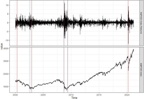
The information criterion introduced in Section 2.2 selects nine factors (with appropriate transformation), that is, $\widehat{q}=9$. We set ${\Delta }_n=20$ and $M_n^c=M_n^e=1000$ in the WBS-Cov and WSBS-Cov algorithms. Combined with SSIC, the WBS-Cov algorithm detects five breaks in the covariance matrix of the common components, and the WSBS-Cov algorithm detects three breaks in the idiosyncratic components. We plot the estimated break times on the series of the S&P 500 index and its returns in Figure 1, where the red vertical lines denote breaks in the common components and the blue dotted vertical lines denote breaks in the idiosyncratic components. Among the five breaks in the common components, two occur during the period of a bearish market from 2000 to 2003, two occur in 2008 and 2009 during the global financial crisis, and one occurs recently due to the COVID-19 outbreak. Among the three breaks in the idiosyncratic errors, the first break occurs around the end of 2002, the second and third breaks occur in 2008 and 2009.

Fig. 1 The detected break times in the covariance structure of the 375 daily returns of the S&P 500 constituents from January 01, 2000 to February 28, 2021. The estimated break dates for common components are April 24, 2000, November 25, 2002, September 12, 2008, May 08, 2009 and March 06, 2020 (in red lines); and the estimated break dates for idiosyncratic components are August 06, 2002, September 11, 2008 and May 11, 2009 (in blue dotted lines).

6.2 Calibration

We next provide a simulation using the factor model with calibrated parameters from the empirical study, and aim to further examine the proposed break detection methods in finite samples.

• Generate a simulated dataset with n = 5322 and d = 375 as the real data.

• Consider six sub-periods separated by the five estimated break dates in the common components (see the red lines in Figure 1) and use the PCA estimated factor loadings. The factors are drawn from a standard normal distribution independently over time and across dimension.

• Divide the estimated idiosyncratic errors into four segments split by the three estimated breaks in idiosyncratic components (see the blue dotted lines in Figure 1), and separately estimate their sample covariance matrices. For each segment, generate idiosyncratic errors by a multivariate normal distribution independently over time with mean zero and covariance matrix being the sample covariance matrix.

The above generating mechanism guarantees the simulated covariance structure to be the same as that for the empirical data. As in the simulation study in Section 5, we repeat the simulation procedure 100 times and report the break detection results. For simplicity, we fix ${\xi }_n^e=95.99$ in WSBS-Cov, which is calculated by applying the method in Section 4 to the real data. Table 3 reports the average break number estimates, the number of times that the estimated break is within a distance of $\text{log}\hspace{0.17em}(n)\approx 8.6$ to the true break, denoted as $\text{ACU}$, and the root-mean-squared distance of the closest estimated break to the true break, denoted as $\text{RMSE}$. Except for the first two breaks (April 24, 2000 and November 25, 2002) in the common components, $\text{ACU}$s are larger than 95% and $\text{RMSE}$s are smaller than 4, indicating that the break dates are accurately detected. The low $\text{ACU}$s and large $\text{RMSE}$s of the first two breaks may be due to the relatively weak break magnitude. The estimated break numbers reported in Table 3 are slightly larger than the true break numbers (5 for the common components and 3 for the idiosyncratic components). In addition, we also fix $q_0=12$ in the break detection procedures and obtain similar simulation results, showing that the proposed methods work when the factor number is over-estimated.

Table 3 Detection results on calibrated data.

	W(S)BS-Cov 5.01 3.31		W(S)BS-Cov (fix $q_0=12$) 5.02 3.08
Mean ${\widehat{K}}_1$
Mean ${\widehat{K}}_2$
	$\text{ACU}(\%)$	$\text{RMSE}$	$\text{ACU}(\%)$	$\text{RMSE}$
Breaks in common components
24/04/2000	79	8.721	79	8.731
25/11/2002	88	5.725	85	6.813
12/09/2008	99	1.643	100	1.300
08/05/2009	99	2.502	99	2.240
06/03/2020	97	3.838	97	3.929
Breaks in idiosyncratic error components
06/08/2002	97	3.425	96	2.466
11/09/2008	100	1.503	100	1.562
11/05/2009	99	2.995	99	1.912

6.3 Comparison with Observed Risk Factors

As a benchmark, we also download eight observable risk factors (over January 01, 2000–February 28, 2021) from Kenneth R. French’s data library¹ and study breaks in their covariance structure. These risk factors include the excess return (MKT), the size factor (SMB), the value factor (HML), the profitability factor (RMW) and the investment factor (CMA) introduced by Fama and French (1993, 2015); the Momentum factor (MOM) proposed by Carhart (1997) in a four-factor model; and the short term reversal factor (STRev) and the long-term reversal factor (LTRev) which are less famous but equally important (see De Bondt and Thaler 1987; Lehmann 1990). They are often used as observable proxies of latent factors in the approximate factor model. We plot patterns of observed factors in Figure 2, from which we can see that they vary drastically during the global financial crisis and the COVID-19 outbreak. Let ${\mathit{Z}}_t={(Z_{1t},\dots ,Z_{8t})}^{\mathrm{⊺}}$ denote the vector containing the eight risk factors, $t=1,\dots ,5322$. As the dimension of ${\mathit{Z}}_t$ is low, there is no need to impose the approximate factor model framework. Using the WBS-Cov algorithm (without any latent factor structure) in Section 2.3, we detect five break dates: April 19, 2001, July 01, 2008, September 12, 2008, May 13, 2009 and March 06, 2020. Note that the first two estimated break dates (April 19, 2001 and July 01, 2008) are quite different from the first two break dates (April 24, 2000 and November 25, 2002) in the common components obtained by applying the proposed WBS-Cov to the estimated factors, see Figure 1. Table 4 shows the canonical correlation between the estimated factors and observed factors for the entire sample and six subsamples divided by the estimated break dates in the common components. p-values are reported in the brackets using the F-approximations of Rao’s test statistic related to Wilks’ Lambda (see Rao 1973). Some of the minimum canonical correlations are small and insignificant, indicating that the space spanned by the eight observed factors may be not the same as that spanned by the nine PCA estimated factors.

Fig. 2 Variation of eight commonly used risk factors from January 01, 2000 to February 28, 2021. The estimated break dates are April 19, 2001, July 01, 2008, September 12, 2008, May 13, 2009 and March 06, 2020 (in red lines).

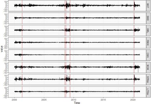
Table 4 Canonical correlation between estimated factors and observed factors.

	Period 1	Period 2	Period 3	Period 4	Period 5	Period 6	Total
From	01/01/2000	25/04/2000	26/11/2002	13/09/2008	09/05/2009	07/03/2020	01/01/2000
To	24/04/2000	25/11/2002	12/09/2008	08/05/2009	06/03/2020	28/02/2021	28/02/2021
First	0.988	0.984	0.993	0.998	0.994	0.996	0.990
p-value 1:8	(0.000)	(0.000)	(0.000)	(0.000)	(0.000)	(0.000)	(0.000)
Second	0.964	0.898	0.873	0.947	0.861	0.949	0.850
p-value 2:8	(0.000)	(0.000)	(0.000)	(0.000)	(0.000)	(0.000)	(0.000)
Third	0.742	0.588	0.817	0.877	0.651	0.784	0.726
p-value 3:8	(0.000)	(0.000)	(0.000)	(0.000)	(0.000)	(0.000)	(0.000)
Fourth	0.605	0.508	0.627	0.760	0.553	0.577	0.554
p-value 4:8	(0.000)	(0.000)	(0.000)	(0.000)	(0.000)	(0.000)	(0.000)
Fifth	0.517	0.359	0.444	0.615	0.384	0.383	0.292
p-value 5:8	(0.007)	(0.000)	(0.000)	(0.000)	(0.000)	(0.000)	(0.000)
Sixth	0.418	0.280	0.239	0.431	0.256	0.308	0.207
p-value 6:8	(0.129)	(0.000)	(0.000)	(0.000)	(0.000)	(0.000)	(0.000)
Seventh	0.259	0.107	0.134	0.398	0.155	0.219	0.119
p-value 7:8	(0.605)	(0.255)	(0.000)	(0.000)	(0.000)	(0.007)	(0.000)
Eighth	0.051	0.027	0.087	0.256	0.022	0.160	0.039
p-value 8:8	(0.916)	(0.795)	(0.004)	(0.005)	(0.510)	(0.047)	(0.019)

NOTE: p-values are reported in the brackets using the F-approximations of Rao’s test statistics related to Wilks’ Lambda.

To further analyze whether breaks in the common components can be explained by the observed factors, we run regression of stock returns on the eight observed factors and detect whether breaks exist in covariances of the regression residuals. We apply the factor model (2.2) to the residual vectors and use the information criterion to select six factors. Using WBS-Cov, we detect six breaks in the common components (of the residual vectors): April 20, 2000, November 22, 2002, July 07, 2008, September 26, 2008, May 08, 2009 and March 06, 2020, and one break in the idiosyncratic components which is August 12, 2002. Note that the first two breaks in the common components April 20, 2000 and November 22, 2002 are very close to April 24, 2000 and November 25, 2002, respectively, which are reported in Figure 1. Hence, we may conclude that break detection of a low-dimensional observed risk factor cannot fully capture structural breaks in covariance of price changes in the entire stock market.

7 Conclusion

In this article, we detect and estimate multiple structural breaks in the contemporaneous covariance structure of the high-dimensional time series vector. We allow high correlation between the time series variables by imposing the approximate factor model, a commonly-used framework in economics and finance. The structural breaks occur in either the common or idiosyncratic error components. When there are breaks in the factor loadings or factor numbers, we transform the factor model in order to make the classic PCA method applicable and subsequently obtain estimates of the transformed factors and approximation of the idiosyncratic errors. The construction of the CUSUM quantities is based on the second-order moments of the estimated factors and errors. The WBS algorithm introduced by Fryzlewicz (2014), combined with SSIC, is extended to the multivariate setting to detect breaks in covariance structure of the common components, estimating the location and number of breaks. For the idiosyncratic error components, we combine the WBS-Cov algorithm and the sparsified CUSUM statistic to detect structural breaks (which can be either sparse or dense), extending the SBS algorithm proposed by Cho and Fryzlewicz (2015). Under some regularity conditions, we show consistency of the estimated break numbers and derive the near-optimal rates (up to a fourth-order logarithmic factor) for the estimated breaks. Monte Carlo simulation studies are conducted to examine the numerical performance of the proposed WBS-Cov and WSBS-Cov methods in finite samples and its comparison with the method introduced by Barigozzi, Cho, and Fryzlewicz (2018). In addition, we examine performance of the proposed methods when breaks are on weak factors. In the empirical application to the return series of S&P 500 constituent, we detect five break in the common components and three breaks in the idiosyncratic error components by the developed methods.

Acknowledgments

The authors would like to thank an Associate Editor and two reviewers for the constructive comments, which helped to improve the article.

Supplementary Materials

The supplementary materials contains the detailed proofs of the main asymptotic results, a simple motivating example for the factor model transformation as well as additional simulation studies.

Additional information

Funding

The second author’s research was partly supported by the BA/Leverhulme Small Research Grant funded by the Leverhulme Trust (No. SRG1920/100603). The third author’s research was supported by the Engineering and Physical Sciences Research Council (No. EP/L014246/1).

Notes

1 http://mba.tuck.dartmouth.edu/pages/faculty/ken.french/data_library.html.

Appendix A:

Technical Assumptions

The following assumptions are needed to establish the asymptotic theorems in Sections 3.1 and 3.2. Some of the conditions (such as the moment conditions) may be not the weakest possible but can be relaxed at the cost of more lengthy proofs.

Assumption 1.

1. For each $k=1,\dots ,K_1+1$, the process $\{({\mathit{F}}_{t,k},{\mathit{ϵ}}_t)\}$ is α-mixing dependent with the mixing coefficient ${\alpha }_k(·)$ satisfying$$\underset{1\le k\le K_1+1}{\max }{\alpha }_k(s)\mathrm{\asymp }{\rho }^s,0<\rho <1.$$

2. For $k=1,\dots ,K_1+1$ and $j=1,\dots ,d,\mathrm{E}[{\mathit{F}}_{t,k}]=\mathbf{0},\mathrm{E}[{\mathit{ϵ}}_t]=\mathbf{0}$ and $\mathrm{E}[{\mathrm{ϵ}}_{tj}{\mathit{F}}_{t,k}]=\mathbf{0}$. In addition,$$\underset{1\le k\le K_1+1}{\max }\underset{{\eta }_{k-1}^c+1\le t\le {\eta }_k^c}{\max }\mathrm{E}\left[\right|\left|{\mathit{F}}_{t,k}\right|{|}_2^{{\delta }_F}]<\infty ,\underset{1\le t\le n}{\max }\underset{1\le j\le d}{\max }\mathrm{E}[\left|{\mathrm{ϵ}}_{tj}{|}^{{\delta }_{\mathrm{ϵ}}}\right]<\infty ,$$

where ${\delta }_F>2$ and ${\delta }_{\mathrm{ϵ}}>2$.

Assumption 2.

1. For $k=1,\dots ,K_1+1$, the covariance matrix $\text{cov}({\mathit{F}}_{t,k})={\mathbf{\Sigma }}_{F,k}$ of the latent factors when ${\eta }_{k-1}^c+1\le t\le {\eta }_k^c$, is $r_k\times r_k$ positive definite. The positive integers K₁ and r_k, $k=1,\dots ,K_1+1$, are all bounded.

2. Letting ${\lambda }_{k,j}^0$ be the jth factor loading vector of ${\mathbf{\Lambda }}_k^0$ defined in (2.2), $\left|\right|{\lambda }_{k,j}^0|{|}_2$ is bounded from above uniformly over $j=1,\dots ,d$ and $k=1,\dots ,K_1+1$. In addition, letting $\overline{\mathbf{\Lambda }}=\left[{\mathbf{\Lambda }}_1^0,\dots ,{\mathbf{\Lambda }}_{K_1+1}^0\right]$ which is a $d\times {\sum }_{k=1}^{K_1+1}{r}_k$ matrix, the column rank of $\overline{\mathbf{\Lambda }}$ is q₀ and there exist positive constants $\underset{¯}{\mu }$ and $\overline{\mu }$ such that

$0<\underset{¯}{\mu }\le {\mu }_{q_0}\left(\frac{1}{d}{\overline{\mathbf{\Lambda }}}^{\mathrm{⊺}}\overline{\mathbf{\Lambda }}\right)\le {\mu }_1\left(\frac{1}{d}{\overline{\mathbf{\Lambda }}}^{\mathrm{⊺}}\overline{\mathbf{\Lambda }}\right)\le \overline{\mu }<\infty .$(A.1)

Assumption 3.

1. There exists a positive constant ι₀ such that

$\underset{1\le k\le K_1+1}{\max }\underset{1\le t\le n}{\max }\mathrm{E}\left[{\Vert {\sum }_{j=1}^d{\lambda }_{k,j}^0{\mathrm{ϵ}}_{tj}\Vert }_2^{{\delta }_{\mathrm{ϵ}}}\right]\le {\iota }_0·d^{{\delta }_{\mathrm{ϵ}}/2}$(A.2)and

$\underset{1\le s,t\le n}{\max }\mathrm{E}\left[{\left|{\sum }_{j=1}^d\left\{{\mathrm{ϵ}}_{sj}{\mathrm{ϵ}}_{tj}-\mathrm{E}\left[{\mathrm{ϵ}}_{sj}{\mathrm{ϵ}}_{tj}\right]\right\}\right|}^{{\delta }_{\mathrm{ϵ}}}\right]\le {\iota }_0·d^{{\delta }_{\mathrm{ϵ}}/2}.$(A.3)

1. There exists a positive constant ${\iota }_1>0$ such that

$\underset{1\le j\le d}{\max }\underset{1\le t\le n}{\max }\mathrm{E}\left[\text{exp}\hspace{0.17em}\left\{{\iota }_1{\mathrm{ϵ}}_{tj}^2\right\}\right]<\infty ,\underset{1\le k\le K_1+1}{\max }\underset{{\eta }_{k-1}^c+1\le t\le {\eta }_k^c}{\max }\mathrm{E}\left[\text{exp}\hspace{0.17em}\left\{{\iota }_1\left|\right|{\mathit{F}}_{t,k}|{|}_2^2\right\}\right]<\infty .$(A.4)

Assumption 4.

1. There exist positive constants ι₂, ι₃, and ϑ such that$${\iota }_2\hspace{0.17em}{\text{log}}^{5+\vartheta }(d)\le n\le {\iota }_3{d}^{\delta /(\delta +4)},$$

where $\delta ={\delta }_F\wedge {\delta }_{\mathrm{ϵ}}$.

1. Letting ${\kappa }_n^c={\min }_{1\le k\le K_1+1}({\eta }_k^c-{\eta }_{k-1}^c)$,$${\underset{¯}{\omega }}_n^c=\frac{1}{d^2}·\underset{1\le k\le K_1}{\min }{\Vert {\mathbf{\Sigma }}_{k+1}^0(\mathbf{\Lambda },\mathit{F})-{\mathbf{\Sigma }}_k^0(\mathbf{\Lambda },\mathit{F})\Vert }_F^2$$

and $${\overline{\omega }}_n^c=\frac{1}{d^2}·\underset{1\le k\le K_1}{\max }{\Vert {\mathbf{\Sigma }}_{k+1}^0(\mathbf{\Lambda },\mathit{F})-{\mathbf{\Sigma }}_k^0(\mathbf{\Lambda },\mathit{F})\Vert }_F^2,$$ we have$${\kappa }_n^c\mathrm{\asymp }n,\frac{{\underset{¯}{\omega }}_n^c}{{\overline{\omega }}_n^c}·\frac{{\kappa }_n^c{\underset{¯}{\omega }}_n^c}{\hspace{0.17em}{\text{log}}^{4}n}\to \infty ,M_n^c\to \infty ,$$ where $M_n^c$ is the number of random intervals drawn in the WBS-Cov algorithm.

1. Letting ${\kappa }_n^e={\min }_{1\le k\le K_2+1}({\eta }_k^e-{\eta }_{k-1}^e)$,$$\begin{array}{c}{\underset{¯}{\omega }}_n^e=\underset{1\le k\le K_2}{\min }\underset{(i,j)\in {\mathcal{I}}_k}{\min }{\left|{\sigma }_{k+1|i,j}^e-{\sigma }_{k|i,j}^e\right|}^2,\\ {\overline{\omega }}_n^e=\underset{1\le k\le K_2}{\max }\underset{(i,j)\in {\mathcal{I}}_k}{\max }{\left|{\sigma }_{k+1|i,j}^e-{\sigma }_{k|i,j}^e\right|}^2,\end{array}$$

where ${\mathcal{I}}_k=\left\{(i,j):{\sigma }_{k+1|i,j}^e\ne {\sigma }_{k|i,j}^e,1\le i,j\le d\right\}$ and ${\sigma }_{k|i,j}^e$ is the (i, j)-entry of ${\mathbf{\Sigma }}_k^0(\mathit{ϵ})$, we have$${\overline{\omega }}_n^e\mathrm{\asymp }{\underset{¯}{\omega }}_n^e,\frac{{\kappa }_n^e{\underset{¯}{\omega }}_n^e}{\hspace{0.17em}{\text{log}}^4(nd)}·{\left(\frac{{\kappa }_n^e}{n}\right)}^4\to \infty ,{\left[1-{\left({\kappa }_n^e/(3n)\right)}^2\right]}^{M_n^e}\to 0,$$

where $M_n^e$ is the number of random intervals drawn in the WSBS-Cov algorithm.

Assumption 5.

There exist $0<\underset{¯}{\sigma }<\overline{\sigma }<\infty$ such that$$\underset{¯}{\sigma }\le \underset{(l,u):1\le l<u\le n}{\min }\underset{1\le i,j\le d}{\min }{\widehat{\sigma }}_{l,u}(i,j)\le \underset{(l,u):1\le l<u\le n}{\max }\underset{1\le i,j\le d}{\max }{\widehat{\sigma }}_{l,u}(i,j)\le \overline{\sigma }$$with probability approaching one, where ${\widehat{\sigma }}_{l,u}(i,j)$ is defined in (2.12). In addition, ${\widehat{\sigma }}_{l,u}(i,j)={\widehat{\sigma }}_{l,u}(j,i)$.

The assumption of mixing dependence on the latent common factor and idiosyncratic error process in Assumption 1(i) is very mild and covers some commonly-used vector time series models. Note that the α-mixing dependence condition allows the underlying process to be nonstationary with time-varying covariance structure (e.g., the piece-wise stationary time series process with breaks in the covariance matrix). The moment conditions in Assumptions 1(ii) and 3 are crucial to consistently estimate the factors and factor loadings (with rotation) in the transformed factor model (2.4).

Assumption 2 contains some fundamental conditions for the approximate factor model (2.2), which can be seen as a generalized version of those for the stable factor model without breaks (e.g., Bai and Ng 2002; Fan, Liao, and Mincheva 2013). These conditions, together with ${\kappa }_n^c\mathrm{\asymp }n$ in Assumption 4(ii), indicate that there exists a nonsingular limiting matrix for $\frac{1}{n}{\sum }_{t=1}^n{\mathit{F}}_t^{\mathrm{\star }}{\mathit{F}}_t^{\mathrm{\star ⊺}}$ and ${\mathbf{\Lambda }}^{\mathrm{\star }}$ is of full column rank (see Proposition 3.1), which are essential to derive the convergence result for the PCA estimated factors and factor loadings. In addition, Assumption 2 also guarantees that ${\overline{\omega }}_n^c=O(1)$.

The moment conditions (A.2) and (A.3) in Assumption 3(i) imply that the idiosyncratic errors ϵ_tj are allowed to be weakly dependent over j. Similar high-level moment conditions can be found in Assumption 4 in Bai and Ng (2002) and Assumption 3.4 in Fan, Liao, and Mincheva (2013). Assumption 3(ii) is similar to the exponential-tail condition commonly used in high-dimensional data analysis and is needed to allow the dimension d to be divergent at an exponential rate of n.

Assumption 4(i) indicates that both d and n diverge to infinity jointly, which is a typical large panel data setting necessary for consistent estimates of the rotated factors and factor loadings. A very similar assumption is also used in Theorem 1 of Fan, Liao, and Mincheva (2013). In particular, Assumption 4(i) shows that d can be divergent to infinity at an exponential rate of n, further relaxing the corresponding condition assumed in Barigozzi, Cho, and Fryzlewicz (2018) and Wang, Yu, and Rinaldo (2021). Although the restriction $n\le {\iota }_3{d}^{\delta /(\delta +4)}$ indicates that n is of smaller asymptotic order than d, our methodology is still applicable if n is much larger than d by switching the role of n and d and the role of the factor loadings and common factors in the PCA estimation (see sec. 3 in Bai and Li 2012). Assumption 4(ii) is mainly used for the asymptotics of WBS-Cov in the common components, and would be automatically satisfied when ${\iota }_4\le {\underset{¯}{\omega }}_n^c\le {\overline{\omega }}_n^c\le {\iota }_5$ and $M_n^c=\lfloor \hspace{0.17em}\text{log}\hspace{0.17em}n\rfloor$, where ${\iota }_4<{\iota }_5$ are two positive constants. Assumption 4(iii) is mainly used to derive the WSBS-Cov asymptotic theory in the idiosyncratic error components. The restriction ${\overline{\omega }}_n^e\mathrm{\asymp }{\underset{¯}{\omega }}_n^e$ is only imposed to facilitate the proofs. The restrictions on ${\underset{¯}{\omega }}_n^c$ and ${\underset{¯}{\omega }}_n^e$ are consistent with the argument in Andrews (1993) and Bai (1997) that the break points can be identified only if the size of breaks, that is, ${({\underset{¯}{\omega }}_n^c)}^{1/2}$ and ${({\underset{¯}{\omega }}_n^e)}^{1/2}$ in our article, is asymptotically larger than $n^{-1/2}$. Assumption 4(iii) also indicates that there might be more frequent breaks in the idiosyncratic error components than in the common components, and the restriction $\frac{{\kappa }_n^e{\underset{¯}{\omega }}_n^e}{\hspace{0.17em}{\text{log}}^4(nd)}·{\left(\frac{{\kappa }_n^e}{n}\right)}^4\to \infty$ would be automatically satisfied when ${\kappa }_n^e\mathrm{\asymp }{n}^{\Theta }$ and $\left({\underset{¯}{\omega }}_n^e{n}^{5\Theta -4}\right)/\hspace{0.17em}{\text{log}}^4(nd)\to \infty$ with $\Theta \in (4/5,1]$. In contrast, the minimum length ${\kappa }_n^c$ of the subintervals separated by break points in the common components is of order n. Assumption 5 requires the random normalizers in the WSBS-Cov to be uniformly bounded away from zero and infinity with probability approaching one.

In Assumption 2(i), we assume that K₁ and r_k, $k=1,\dots ,K_1$, are all bounded, which indicates that q₀, the number of transformed factors in (2.4), is upper bounded by Proposition 2.1. This assumption facilitates proofs of the consistent estimation theory for the transformed factors and factor loadings and consistent break estimation theory. It would be an interesting extension by allowing the break numbers K₁ and K₂ to grow slowly as $n\to \infty$. In this case, q₀ would be divergent as well, and the condition of ${\kappa }_n^c\mathrm{\asymp }n$ would be violated. Consequently, we need to amend the estimation and break detection techniques, and modify some technical assumptions (such as Assumption 4) and the asymptotic proofs. We will further explore this in our future study.

References

- Alessi, L., Barigozzi, M., and Capasso, M. (2010), “Improved Penalization for Determining the Number of Factors in Approximate Factor Models,” Statistics and Probability Letters, 80, 1806–1813. DOI: 10.1016/j.spl.2010.08.005.
- Andrews, D. W. (1993), “Tests for Parameter Instability and Structural Change with Unknown Change Point,” Econometrica, 61, 821–856. DOI: 10.2307/2951764.
- Anderson, T. W. (2003), An Introduction to Multivariate Statistical Analysis, Wiley Series in Probability and Statistics (3rd ed.), New York: Wiley.
- Aston, J. A., and Kirch, C. (2018), “High Dimensional Efficiency with Applications to Change Point Tests,” Electronic Journal of Statistics, 12, 1901–1947. DOI: 10.1214/18-EJS1442.
- Aue, A., Hörmann, Horváth, L., and Reimherr, M. (2009), “Break Detection in the Covariance Structure of Multivariate Time Series Models,” Annals of Statistics, 37, 4046–4087.
- Bai, J. (1997), “Estimating Multiple Breaks on at a Time,” Econometric Theory, 13, 315–352. DOI: 10.1017/S0266466600005831.
- Bai, J., Han, X., and Shi, Y. 2020, “Estimation and Inference of Change Points in High-Dimensional Factor Models,” Journal of Econometrics, 219, 66–100 DOI: 10.1016/j.jeconom.2019.08.013.
- Bai, J., and Li, K. (2012), “Statistical Analysis of Factor Models of High Dimension,” Annals of Statistics, 40, 436–465.
- Bai, J., and Ng, S. (2002), “Determining the Number of Factors in Approximate Factor Models,” Econometrica, 70, 191–221. DOI: 10.1111/1468-0262.00273.
- Bai, J., and Ng, S- (2006), “Confidence Intervals for Diffusion Index Forecasts and Inference for Factor-Augmented Regressions,” Econometrica, 74, 1135–1150.
- Baltagi, B., Kao, C., and Wang, F. (2017), “Identification and Estimation of a Large Factor Model with Structural Instability,” Journal of Econometrics, 197, 87–100. DOI: 10.1016/j.jeconom.2016.10.007.
- Baltagi, B., Kao, C., and Wang, F. (2021), “Estimating and Testing High Dimensional Factor Models with Multiple Structural Changes,” Journal of Econometrics, 220, 349–365.
- Barigozzi, M., Cho, H., and Fryzlewicz, P. (2018), “Simultaneous Multiple Change-Point and Factor Analysis for High-Dimensional Time Series,” Journal of Econometrics, 206, 187–225. DOI: 10.1016/j.jeconom.2018.05.003.
- Bickel, P., and Levina, E. (2008a), “Covariance Regularization by Thresholding,” Annals of Statistics, 36, 2577–2604.
- Bickel, P., and Levina, E(2008b), “Regularized Estimation of Large Covariance Matrices,” Annals of Statistics, 36, 199–227.
- Breitung, J., and Eickmeier, S. (2011), “Testing for Structural Breaks in Dynamic Factor Models,” Journal of Econometrics, 163, 71–84. DOI: 10.1016/j.jeconom.2010.11.008.
- Cai, T. T., and Liu, W. (2011), “Adaptive Thresholding for Sparse Covariance Matrix Estimation,” Journal of the American Statistical Association, 106, 672–684. DOI: 10.1198/jasa.2011.tm10560.
- Cai, T. T., Ren, Z., and Zhou, H. (2016), “Estimating Structured High-Dimensional Covariance and Precision Matrices: Optimal Rates and Adaptive Estimation,” Electronic Journal of Statistics, 10, 1–59.
- Carhart, M. M. (1997), “On Persistence in Mutual Fund Performance,” Journal of Finance, 52, 57–82. DOI: 10.1111/j.1540-6261.1997.tb03808.x.
- Chamberlain, G., and Rothschild, M. (1983), “Arbitrage, Factor Structure and Mean-Variance Analysis in Large Asset Markets,” Econometrica, 51, 1305–1324. DOI: 10.2307/1912276.
- Chen, J., Li, D., Linton, O., and Lu, Z. (2018), “Semiparametric Ultra-High Dimensional Model Averaging of Nonlinear Dynamic Time Series,” Journal of the American Statistical Association, 113, 919–932. DOI: 10.1080/01621459.2017.1302339.
- Chen, L., Dolado, J. J., and Gonzalo, J. (2013), “Detecting Big Structural Breaks in Large Factor Models,” Journal of Econometrics, 180, 30–48. DOI: 10.1016/j.jeconom.2014.01.006.
- Chen, X., Xu, M., and Wu, W. (2013), “Covariance and Precision Matrix Estimation for High-Dimensional Time Series,” Annals of Statistics, 41, 2994–3021.
- Chen, Z., and Leng, C. (2016), “Dynamic Covariance Models,” Journal of the American Statistical Association, 111, 1196–1207. DOI: 10.1080/01621459.2015.1077712.
- Cheng, X., Liao, Z., and Schorfheide, F. (2016), “Shrinkage Estimation of High-Dimensional Factor Models with Structural Instabilities,” Review of Economic Studies, 83, 1511–1543. DOI: 10.1093/restud/rdw005.
- Cho, H. (2016), “Change-Point Detection in Panel Data via Double CUSUM Statistic,” Electronic Journal of Statistics, 10, 2000–2038. DOI: 10.1214/16-EJS1155.
- Cho, H., and Fryzlewicz P. (2012), “Multiscale and Multilevel Technique for Consistent Segmentation of Nonstationary Time Series,” Statistica Sinica, 22, 207–229. DOI: 10.5705/ss.2009.280.
- Cho, H., and Fryzlewicz P. (2015), “Multiple Change-Point Detection for High-Dimensional Time Series via Sparsified Binary Segmentation,” Journal of the Royal Statistical Society, Series B, 77, 475–507.
- De Bondt, W. F., and Thaler, R. H. (1987), “Further Evidence on Investor Overreaction and Stock Market Seasonality,” Journal of Finance, 42, 557–581. DOI: 10.1111/j.1540-6261.1987.tb04569.x.
- Duan, J., Bai, J., and Han, X. (2022), “Quasi-Maximum Likelihood Estimation of Break Point in High-Dimensional Factor Mmodels,” Journal of Econometrics, forthcoming. DOI: 10.1016/j.jeconom.2021.12.011.
- El Karoui, N. (2008a), “Operator Norm Consistent Estimation of Large-Dimensional Sparse Covariance Matrices,” Annals of Statistics, 36, 2717–2756.
- El Karoui, N. - (2008b), “Spectrum Estimation for Large Dimensional Covariance Matrices Using Random Matrix Theory,” Annals of Statistics, 36, 2757–2790.
- Fama, E. F., and French, K. (1992), “The Cross-Section of Expected Stock Returns,” Journal of Finance, 47, 427–465. DOI: 10.1111/j.1540-6261.1992.tb04398.x.
- Fama, E. F., and French, K. (1993), “Common Risk Factors in the Returns on Stocks and Bonds,” Journal of Financial Economics, 33, 3–56.
- Fama, E. F., and French, K. (2015), “A Five-Factor Asset Pricing Model,” Journal of Financial Economics, 116, 1–22.
- Fan, J., Liao, Y., and Liu, H. (2016), “An Overview on the Estimation of Large Covariance and Precision Matrices,” Econometrics Journal, 19, 1–32.
- Fan, J., Liao, Y., and Mincheva, M. (2013), “Large Covariance Estimation by Thresholding Principal Orthogonal Complements,” (with discussion), Journal of the Royal Statistical Society, Series B, 75, 603–680. DOI: 10.1111/rssb.12016.
- Freyaldenhoven, S. (2022), “Factor Models with Local Factors – Determining the Number of Relevant Factors,” Journal of Econometrics, 229, 80–102. DOI: 10.1016/j.jeconom.2021.04.006.
- Fryzlewicz, P. (2014), “Wild Binary Segmentation for Multiple Change-Point Detection,” Annals of Statistics, 42, 2243–2281.
- Fryzlewicz, P (2020), “Detecting Possibly Frequent Change-Points: Wild Binary Segmentation 2 and Steepest-Drop Model Selection,” Journal of the Korean Statistical Society, 49, 1027–1070.
- Han X., and Inoue, A. (2015), “Tests for Parameter Instability in Dynamic Factor Models,” Econometric Theory, 31, 1117–1152. DOI: 10.1017/S0266466614000486.
- Hariz, S. B., Wylie, J. J., and Zhang, Q. (2007), “Optimal Rate of Convergence for Nonparametric Change-Point Estimators for Nonstationary Sequences,” Annals of Statistics, 35, 1802–1826.
- Huang, N., and Fryzlewicz, P. (2019), “NOVELIST Estimator of Large Correlation and Covariance Matrices and their Inverses,” Test, 28, 694–727. DOI: 10.1007/s11749-018-0592-4.
- Jirak, M. (2015), “Uniform Change Point Tests in High Dimension,” Annals of Statistics, 43, 2451–2483.
- Killick, R., Fearnhead, P., and Eckley, I. (2012), “Optimal Detection of Changepoints with a Linear Computational Cost,” Journal of the American Statistical Association, 107, 1590–1598. DOI: 10.1080/01621459.2012.737745.
- Korkas, K. K., and Fryzlewicz, P. (2017), “Multiple Change-Point Detection for Non-stationary Time Series Using Wild Binary Segmentation,” Statistica Sinica, 27, 287–311. DOI: 10.5705/ss.202015.0262.
- Korostelev, A.P. (1988), “On Minimax Estimation of a Discontinuous Signal,” Theory of Probability & Its Applications, 32, 727–730.
- Lam, C., and Fan, J. (2009), “Sparsity and Rates of Convergence in Large Covariance Matrix Estimation,” Annals of Statistics, 37, 4254–4278.
- Ledoit, O., and Wolf, M. (2004), “A Well-Conditioned Estimator for Large-Dimensional Covariance Matrices,” Journal of Multivariate Analysis, 88, 365–411. DOI: 10.1016/S0047-259X(03)00096-4.
- Lehmann, B. N. (1990), “Fads, Martingales, and Market Efficiency,” Quarterly Journal of Economics, 105, 1–28. DOI: 10.2307/2937816.
- Li, J., Todorov, V., Tauchen, G., and Lin, H. (2019), “Rank Tests at Jump Events,” Journal of Business & Economic Statistics, 37, 312–321.
- Ma, S., and Su, L. (2018), “Estimation of Large Dimensional Factor Models with an Unknown Number of Breaks,” Journal of Econometrics, 207, 1–29. DOI: 10.1016/j.jeconom.2018.06.019.
- Pourahmadi, M. (2013), High-Dimensional Covariance Estimation: With High-Dimensional Data, Hoboken, NJ: Wiley.
- Rao, C. R (1973), Linear Statistical Inference and Its Applications, (2nd ed.), New York: Wiley.
- Rothman, A. J., Levina, E., and Zhu, J. (2009), “Generalized Thresholding of Large Covariance Matrices,” Journal of the American Statistical Association, 104, 177–186. DOI: 10.1198/jasa.2009.0101.
- Safikhani, A., and Shojaie, A. (2022), “Joint Structural Break Detection and Parameter Estimation in High-Dimensional Non-stationary VAR Models,” Journal of the American Statistical Association, 537, 251–264. DOI: 10.1080/01621459.2020.1770097.
- Stock, J. H., and Watson, M. W. (2002), “Forecasting Using Principal Components from a Large Number of Predictors,” Journal of the American Statistical Association 97, 1167–1179. DOI: 10.1198/016214502388618960.
- Venkatraman, E. S. (1992), “Consistency Results in Multiple Change-Point Problems,” Technical Report No. 24, Department of Statistics, Stanford University.
- Vostrikova L. Y. (1981), “Detecting Disorder in Multidimensional Random Processes,” Soviet Mathematics Doklady, 24, 55–59.
- Wang, D., Yu, Y., and Rinaldo, A. (2021), “Optimal Covariance Change Point Localization in High Dimensions,” Bernoulli, 27, 554–575. DOI: 10.3150/20-BEJ1249.
- Wang, D., Yu, Y., Rinaldo, A., and Willett, R. (2019), “Localizing Changes in High-Dimensional Vector Autoregressive Processes,” Working paper. Available at https://arxiv.org/abs/1909.06359.
- Wang, T., and Samworth, R. J. (2018), “High Dimensional Change Point Estimation via Sparse Projection,” Journal of the Royal Statistical Society, Series B, 80, 57–83. DOI: 10.1111/rssb.12243.
- Wu, W., and Pourahmadi, M. (2003), “Nonparametric Estimation of Large Covariance Matrices of Longitudinal Data,” Biometrika, 90, 831–844. DOI: 10.1093/biomet/90.4.831.
- Yu, M., and Chen, X. (2021), “Finite Sample Change Point Inference and Identification for High-Dimensional Mean Vectors,” Journal of the Royal Statistical Society, Series B, 83, 247–270. DOI: 10.1111/rssb.12406.