
 ?Mathematical formulae have been encoded as MathML and are displayed in this HTML version using MathJax in order to improve their display. Uncheck the box to turn MathJax off. This feature requires Javascript. Click on a formula to zoom.
Abstract
We compare two approaches to using information about the signs of structural shocks at specific dates within a structural vector autoregression (SVAR): imposing “narrative restrictions” (NR) on the shock signs in an otherwise set-identified SVAR; and casting the information about the shock signs as a discrete-valued “narrative proxy” (NP) to point-identify the impulse responses. The NP is likely to be “weak” given that the sign of the shock is typically known in a small number of periods, in which case the weak-proxy robust confidence intervals in Montiel Olea, Stock, and Watson are the natural approach to conducting inference. However, we show both theoretically and via Monte Carlo simulations that these confidence intervals have distorted coverage—which may be higher or lower than the nominal level—unless the sign of the shock is known in a large number of periods. Regarding the NR approach, we show that the prior-robust Bayesian credible intervals from Giacomini, Kitagawa, and Read deliver coverage exceeding the nominal level, but which converges toward the nominal level as the number of NR increases.
1 Introduction
Structural vector autoregressions (SVARs) are used in macroeconomics to estimate the dynamic causal effects of structural shocks. A common approach to identifying the effects of these shocks is to impose a set of sign and/or zero restrictions on functions of the SVAR’s structural parameters that together result in set-identification of the parameters of interest (e.g., sign restrictions on impulse responses, as in Uhlig Citation2005). A growing number of papers augment these “traditional” set-identifying restrictions with restrictions that involve the values of the structural shocks in specific periods. For instance, Antolín-Díaz and Rubio-Ramírez (Citation2018) propose restricting the signs of structural shocks based on the historical narrative about the nature of the shocks hitting the economy in particular episodes. An example is the restriction that there was a positive monetary policy shock in the United States in October 1979, which is the year in which the Federal Reserve dramatically raised the federal funds rate following Paul Volcker becoming chairman.1
In this article, we compare two alternative approaches to using information about the signs of structural shocks in specific periods in an SVAR framework. The first approach is to impose the information as restrictions on the signs of the structural shocks in an otherwise set-identified SVAR, as in Antolín-Díaz and Rubio-Ramírez (Citation2018); we refer to this as “shock-sign narrative restrictions” (NR). The second approach follows a suggestion in Plagborg-Møller and Wolf (Citation2021a) that the information about the shock signs could be recast as an external instrument or “proxy” for use in a proxy SVAR (e.g., Mertens and Ravn Citation2013; Stock and Watson Citation2018).2 We refer to this as the “narrative-proxy” (NP) approach.
Following Antolín-Díaz and Rubio-Ramírez (Citation2018), the literature that makes use of NR typically imposes these restrictions within a Bayesian framework.3 This involves specifying a uniform-normal-inverse-Wishart prior over the orthogonal reduced-form parameterization of the SVAR, which is the standard approach in set-identified SVARs (e.g., Arias et al. Citation2018). However, Giacomini, Kitagawa, and Read (Citation2021a)—henceforth, GKR—point out some undesirable features of this approach. Under shock-sign restrictions, the likelihood function possesses flat regions, which implies that a component of the prior is never updated by the data. This raises the concern that posterior inference may be sensitive to the choice of prior.4
To address the issue of posterior sensitivity to the choice of prior under NR, GKR propose applying a variant of the “robust” (multiple-prior) Bayesian approach to inference for set-identified models developed in Giacomini and Kitagawa (Citation2021). This involves replacing the unrevisable component of the prior with a class of priors that are consistent with the identifying restrictions. The class of priors generates a class of posteriors, which can be summarized in various ways. For example, rather than having a single posterior mean, there is a set of posterior means, which is an interval containing every possible posterior mean that could be obtained under the class of priors. One can also report a “robust credible interval,” which is an interval that receives at least a given posterior probability under every posterior in the class of posteriors. This approach eliminates the source of posterior sensitivity arising due to the unrevisable component of the prior. See Giacomini, Kitagawa, and Read (Citation2021b) for a review of robust Bayesian approaches to inference in set-identified econometric models.
As noted in Plagborg-Møller and Wolf (Citation2021a), an alternative way to use information about the signs of a particular structural shock in specific periods is to recast this information as a discrete-valued proxy for the structural shock. Specifically, construct a variable that is equal to one in periods where the shock is known to be positive, minus one in periods where it is known to be negative, and zero in all other periods. This variable is positively correlated with the target structural shock (i.e., “relevant”) and uncorrelated with all other structural shocks (i.e., “exogenous”). The variable is therefore a valid proxy for the structural shock and can be used to point-identify impulse responses to that shock in a proxy SVAR (Mertens and Ravn Citation2013; Stock and Watson Citation2018).5
Montiel Olea, Stock, and Watson (Citation2021)—henceforth, MSW—show that frequentist inference about impulse responses is nonstandard when the proxy variable is only weakly correlated with the target structural shock (see also Lunsford Citation2015). They propose a weak-proxy robust approach to inference, which—under some conditions—has asymptotically valid coverage of the true impulse response regardless of the strength of the correlation between the proxy and shock. We show that the narrative proxy is likely to be weakly correlated with the target structural shock when there are only a small number of periods in which the sign of the shock is known, which tends to be the case empirically; for example, the applications considered in Antolín-Díaz and Rubio-Ramírez (Citation2018) impose NR in no more than a handful of periods. Accordingly, the weak-proxy robust approach to inference is the natural approach to frequentist inference when using NP.
We discuss the frequentist properties of the inferential procedures described above when the parameter of interest is the impulse response to a unit structural shock (e.g., a monetary policy shock that raises the federal funds rate by 100 basis points).6 When the number of NR is fixed with the sample size, we show that the robust credible region has asymptotic frequentist coverage of the true impulse response that is weakly greater than the nominal level. When the number of NR increases proportionally with the sample size, the coverage probability converges to the nominal level asymptotically.
We then show that the assumptions required for the asymptotic validity of the weak-proxy robust confidence intervals in MSW are violated under the NP approach. Specifically, the covariance between the NP and the reduced-form VAR innovations is not -asymptotically normal (where T is the sample size) when the NP is nonzero in a fixed number of periods. The MSW confidence intervals are constructed following the Anderson–Rubin approach, which involves inverting a particular Wald test. The Wald statistic for this test is asymptotically
under the assumptions in MSW. We show that if the NP is nonzero in a fixed number of periods, the null distribution of this test statistic is not
, no matter how large the sample size T is. Consequently, the size of the test with
critical values is generally not equal to the nominal level and the confidence intervals obtained from inverting the test are not guaranteed to attain correct coverage even when T is large. Thus, weak-proxy robust confidence intervals based on the standard Anderson-Rubin approach are not recommended when the NP is nonzero in only a small number of periods.
We provide Monte Carlo evidence in support of our theoretical results. The coverage probability of the weak-proxy robust confidence intervals differs from the nominal level unless the sign of the shock is known in a relatively large number of periods. Whether the intervals under- or over-cover depends on the confidence level. In contrast, the robust credible intervals always over-cover, but the coverage probability converges toward the nominal level as the number of NR increases.
We focus our discussion on a bivariate, static SVAR. The main reason for this simplification is that it allows us to derive an analytical expression for the “conditional identified set” (i.e., the set of parameter values that are consistent with the NR given the reduced-form parameters), which is useful for both illustration and simulation of the NR approach. The theoretical findings do not rely on this simplification, and we provide some suggestions in the article on how the analysis could be generalized to incorporate dynamics or additional variables.
To the best of our knowledge, this is the first article to explore whether information about structural shocks should be used to impose NR in an otherwise set-identified SVAR or to construct a proxy for use in a proxy SVAR. Boer and Lütkepohl (Citation2021) compare the efficiency of proxy SVAR estimators that use only the signs of structural shocks on particular dates against proxies that also use information about the size of the shock (i.e., standard proxies). Based on Monte Carlo simulations, they conclude that the estimator that uses information only about the sign of the shock is nearly as (or, in some cases, more) efficient than the estimator based on the quantitative information. Budnik and Rünstler (Citation2020) consider identification of impulse responses in Bayesian proxy SVARs when the proxy represents the sign of a certain structural shock in particular periods. Their approach to identification departs from the standard proxy SVAR setting and is implemented using linear discriminant analysis or a nonparametric sign-concordance criterion.
The remainder of the article is structured as follows. Section 2 describes the two approaches to using information about shock signs within the context of a stylized SVAR. Section 3 examines the theoretical frequentist properties of the robust Bayesian approach to inference under NR and the weak-proxy robust approach to inference under NP. Section 4 provides results from Monte Carlo simulations supporting the theoretical results. Section 5 concludes.
2 Frameworks for Using Information about Shock Signs
This section introduces a stylized bivariate SVAR and discusses the two approaches to using information about the sign of a structural shock.
2.1 Stylized SVAR
Consider the SVAR(0) for the 2 × 1 vector of endogenous variables :
(1)
(1) where
with
, where
is the 2 × 2 identity matrix. The orthogonal reduced form of the model reparameterizes
as
, where
is the lower-triangular Cholesky factor (with positive diagonal elements) of
. We parameterize
as
(2)
(2)
and denote the vector of reduced-form parameters as
. Q is an orthonormal matrix in the space of 2 × 2 orthonormal matrices,
:
(3)
(3)
where the first set is the set of “rotation” matrices and the second set is the set of “reflection” matrices.
In the absence of any identifying restrictions, the identified set for (the matrix of contemporaneous impulse responses) is
(4)
(4)
The identified set for is then
(5)
(5)
Henceforth, we leave implicit that and we impose the sign normalization
, which is a normalization on the signs of the structural shocks.
The impulse response of the second variable to a shock to the first variable that raises the first variable by one unit is(6)
(6)
In what follows, we assume that this is the parameter of interest.
2.2 Narrative Restrictions and Robust Bayesian Inference
Consider the NR that for some
, which is one of the restrictions proposed by Antolín-Díaz and Rubio-Ramírez (Citation2018) and Ludvigson, Ma, and Ng (Citation2018):
(7)
(7) where
is the first column of the 2 × 2 identity matrix,
. Under the sign normalization and the NR, θ is restricted to the set
(8)
(8)
Since and
enter the inequalities characterizing this set, the NR induces a set-valued mapping from
to θ—and thus to η21 – that depends on the realization of
; GKR refer to this mapping as the “conditional identified set.”7 For example, in the case where
and
, the conditional identified set for θ is
(9)
(9) and the conditional identified set for η21 is
(10)
(10)
The conditional identified set for η21 may be unbounded; for example, when and
, the conditional identified set for θ includes
and the conditional identified set for η21 is
, which implies that the NR is completely uninformative about the impulse response.8
As in GKR, we do not model a mechanism for when the shock-sign restrictions become available. Our analysis assumes that the sign of is revealed in the first K periods, but our results would also hold if we assumed that the sign of
was revealed in K random periods. The set of restrictions can be represented as
. The “unconditional” likelihood based on the sample
and the NR is
(11)
(11) where
is the indicator function equal to one when
and equal to zero otherwise.9 The dependence of the likelihood on θ is only through the indicator functions. The NR truncate the likelihood so that it is flat for any θ satisfying the NR and is zero otherwise, with the points of truncation depending on the realization of
.
The standard approach to Bayesian inference in this setting (e.g., Antolín-Díaz and Rubio-Ramírez Citation2018) would involve specifying a uniform prior over θ, which corresponds to the usual uniform or “Haar” prior over the orthonormal matrix Q (e.g., Baumeister and Hamilton Citation2015; Arias et al. Citation2018). However, GKR argue that the flat likelihood function raises concerns about the sensitivity of posterior inference to the choice of prior, as the posterior for θ will be proportional to the prior whenever the likelihood is nonzero. This is similar to the case under standard sign restrictions (e.g., Baumeister and Hamilton Citation2015). GKR therefore propose extending the robust Bayesian approach of Giacomini and Kitagawa (Citation2021) to this setting.
The key feature of the robust Bayesian approach to inference under NR is that, rather than imposing a single conditional prior over θ, we consider the class of all priors that are consistent with any “traditional” set-identifying restrictions (in this case, the sign normalizations). Combining the class of priors with the unconditional likelihood generates a class of posteriors for θ—and thus for η21—that are consistent with the NR. Importantly, this approach eliminates the source of posterior sensitivity to the unrevisable component of the prior (i.e., the conditional prior for θ given ).
In the current context, the robust Bayesian approach to conducting inference about η21 proceeds as follows. First, impose a prior over and obtain draws of
from its posterior,
. Second, for each draw of
, compute the conditional identified set for η21 given the NR:10
(12)
(12)
(13)
(13)
Finally, using the posterior draws of the bounds of the conditional identified set, construct a robust credible region with credibility α as an interval satisfying
(14)
(14)
This interval receives posterior probability at least α under all posterior distributions within the class of posteriors for η21. The robust credible interval with credibility α will be unbounded whenever .
2.3 Narrative Proxies and Weak-proxy Robust Inference
Plagborg-Møller and Wolf (Citation2021a) suggest that the information about the signs of structural shocks imposed under NR can alternatively be used to construct a proxy variable, which can be used to point-identify impulse responses in a proxy SVAR or instrumental-variable local projection.
Solving the equation for in (1) for
and plugging in (6), we obtain, for
,
(15)
(15) where wt
depends on
, σ11, and θ. To identify the impulse response of interest η21, consider using some variable zt
satisfying
(relevance) and
(exogeneity) as an instrument for
.11 Since
, relevance of zt
implies
. Hence, by the standard identification approach using the linear instrumental-variable method, we can identify η21 by the Wald estimand (Stock and Watson Citation2018):
(16)
(16)
As above, we assume that the sign of the shock is observable in the first K periods. The proposal from Plagborg-Møller and Wolf (Citation2021a) is to use the information about the shock signs to construct zt
as(17)
(17)
is clearly (positively) correlated with
itself and is uncorrelated with
, because the two shocks are independent by assumption. This proxy will therefore satisfy the relevance and exogeneity requirements, and, therefore, at any
, the Wald estimand (16) identifies η21. Since the expectations in (16) are common for all
, a sample analogue estimator for η21 can be formed as
(18)
(18) which is identical to the two-stage least square estimator using zt
as an instrumental variable for
.
In the case where K = 1, . The point estimator of the impulse response will therefore be sensitive to the realization of the structural shocks in a single period (i.e., the period in which the sign of the shock is known). For example, if
and
and
is approximately equal to
(19)
(19) which, rather than the true value of η21, equals the true impulse response of the second variable to the second shock such that the first variable increases by one unit.12 More generally, when K > 1, the estimator of the impulse response under NP may be sensitive to the realizations of the nontarget shocks in the periods in which the sign of the target shock is known.
As discussed in MSW, standard approaches to inference (e.g., based on asymptotic normality of the reduced-form parameters and the delta-method) in proxy SVARs are invalid when the proxy is only weakly correlated with the target structural shock. This is likely to be the case in applications using NP. For example, under the assumption that the structural shocks are normally distributed and the sign of the shock is known in K periods, the expected value of the sample covariance between the proxy variable and the target structural shock is , where T is the number of observations and expectations are taken over alternative realizations of a time series of length T. For K small relative to T, this expected covariance will be close to zero. Furthermore, for K fixed as T approaches infinity, the expected covariance will converge to zero at rate T, which is faster than the
rate of convergence typically considered under weak-instrument asymptotics. The scenario where K is small (or fixed) relative to T appears to be the empirically relevant case given that most studies that impose NR do so in at most a handful of periods.13
Given that the NP is likely to be weakly correlated with the target structural shock in typical empirical applications, it seems natural to turn to the weak-proxy robust approach to inference developed in MSW. Building on the Anderson–Rubin approach to weak-instrument robust inference in microeconometrics, they develop weak-proxy robust confidence intervals for the impulse responses in a proxy SVAR. MSW show that their weak-proxy robust confidence intervals have correct coverage of the true impulse response under the assumption that the reduced-form parameters are asymptotically normally distributed. Importantly, this result does not depend on the strength of the covariance between the NP and the target structural shock.
The Anderson–Rubin confidence intervals are obtained as follows. Define the vector of average covariances between the NP and the observations by(20)
(20)
As noted above, we assume that the sign of is known in the first K periods. This implies that the proxy
is not weakly stationary and the covariance
varies with t:
so
.
Let denote an analogue estimator of
. Because we know the signs of the first structural shock in the first K periods only,
(21)
(21)
The Anderson–Rubin confidence intervals in MSW are constructed by inverting tests based on the Wald statistic(22)
(22) where
is the sample variance-covariance matrix of
. Under the assumptions in MSW,
asymptotically follows the
distribution under the null. Constructing an α-level confidence interval for η21 requires finding the set of values of η21 such that
, where
is the α quantile of the
distribution. This inequality is quadratic in η21 and has an analytical solution.
3 Frequentist Properties of Approaches to Inference
This section discusses the asymptotic frequentist properties of the robust Bayesian approach to inference under NR and the weak-proxy robust approach to inference under NP.
3.1 Robust Bayesian Inference Under NR
GKR show that their robust Bayesian approach to inference under NR is asymptotically valid from a frequentist perspective when the number of NR is fixed with the sample size. In particular, the robust credible interval has at least the nominal level of coverage for the true impulse response to a standard-deviation shock asymptotically under some high-level assumptions. These assumptions are that the conditional identified set for the impulse response is closed and convex, and has lower and upper bounds that are differentiable in at
with nonzero derivatives.14
In the current context, we are interested in the impulse response to a unit shock rather than a standard-deviation shock. As discussed in Read (Citationforthcoming), this shift in the parameter of interest may give rise to an unbounded conditional identified set, depending on and the realization of the data. This means that the asymptotic validity claim from GKR does not immediately apply when the parameter of interest is the impulse response to a unit shock. However, the following informal proof shows that asymptotic validity of the robust credible interval also holds in the NR setting considered in this article.
Conditional on the realization of the data entering the NR, , if the conditional identified set is bounded at any
in an open neighborhood of
and has lower and upper bounds differentiable in
(with nonzero derivatives), the robust credible interval will asymptotically contain the true conditional identified set,
, with probability α under the sampling distribution of the remaining data (i.e.,
). Assuming the NR are correctly specified, the true impulse response will lie within the conditional identified set, so the robust credible interval will also asymptotically contain the true impulse response with probability at least α. If the conditional identified set is unbounded at
and its neighborhood, the robust credible interval is also unbounded with a high probability in terms of the sampling distribution of the remaining data, that is, the robust credible interval contains the true impulse response with probability approaching one under the sampling distribution of the remaining data. Thus, regardless of whether the conditional identified set is bounded around
, the unconditional coverage probability—obtained by averaging over the possible realizations of
—is greater than the nominal coverage probability.
GKR also show that when the number of NR increases with the sample size (i.e., in proportion to
), the posterior distributions of the lower and upper bounds of the conditional identified set for θ are
-consistent for θ0. The posterior consistency property will also carry over to the impulse response η21, in the sense that the posterior distributions of the lower and upper bounds of the conditional identified set for η21 converge to the true η21 so long as
, which are the points of singularity for
. Furthermore, the posteriors of the lower and upper bounds of the conditional identified set for η21 are asymptotically normal, and the posterior credible intervals constructed upon them as well as the robust Bayes credible interval for η21 asymptotically attain the correct frequentist coverage.
3.2 Weak-Proxy Robust Inference Under NP
Assumption 2 of MSW requires that the reduced-form covariance estimator is normally distributed asymptotically. However, in the NP setting with fixed K,
The reduced-form covariance between the NP and the data therefore has a degenerate distribution asymptotically after rescaling by . Consequently, Assumption 2 in MSW is not satisfied, and it is unclear whether the weak-proxy robust confidence intervals will have valid coverage of the true impulse response in the NP setting.
To examine the coverage properties of the Anderson-Rubin confidence intervals in this setting, express the parameter of interest η21 in terms of . η21 is identified by the ratio of the second and first elements of
:
(23)
(23)
Following MSW, we view the Anderson-Rubin confidence intervals as providing inference for the ratio of the two means based on their unbiased statistics . As discussed above, with fixed K,
is not asymptotically normal. In addition, even under the assumption that the structural shocks are Gaussian, the distribution of
is not jointly normal due to the multiplier term
.
As described in Section 2.3, the standard Anderson–Rubin confidence intervals are constructed by inverting a Wald test. Let η21 be the true impulse response specified under the null. If we naively apply the Anderson–Rubin confidence intervals, the Wald statistic for the test to be inverted is given by EquationEquation (22)(22)
(22) .
, which appears in the denominator of the Wald statistic, can be expressed as
(24)
(24)
Multiplying the numerator of the Wald statistic by T yields(25)
(25)
The Wald statistic (22) can then be expressed as(26)
(26)
Under the assumptions in MSW, the Wald statistic has the distribution asymptotically. However, under NP, the expression above for the Wald statistic shows that
does not follow the
distribution under the null even asymptotically as
with fixed K. First, the numerator is not a squared Gaussian random variable when
. Second, the denominator remains random even asymptotically and does not converge in probability to the variance-covariance matrix of the numerator random variable under the null. In the special case where K = 1, the fact that
means that the numerator is a squared Gaussian random variable. However, in this case the denominator is
times the numerator, so the Wald statistic is constant and equal to
under the null. Performing the Wald test using the statistic
and critical values from the
distribution therefore does not generally control the Type I error of the test, because the actual distribution of
is not
. Consequently, a naive application of the Anderson–Rubin confidence intervals is not guaranteed to have the nominal coverage level of the true impulse response.
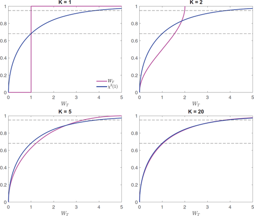
To explore the severity of the distortion of the null distribution of the Wald statistic under NP, plots the null distribution of the Wald statistics under the distributional specification of for different values of K, alongside the
distribution. When K = 1, the Wald statistic is constant and equal to
, so the cumulative distribution function of the Wald statistic is a step function. Since
lies below the 95th percentile of the
distribution (3.84), the 95% Anderson–Rubin confidence intervals span the entire real line and have a coverage probability equal to one. In contrast, since the 68th percentile of the
distribution (0.99) is less than
, the 68% confidence excludes any value of η21 except for
and the intervals have coverage probability equal to zero. As K increases, the null distribution of the Wald statistic converges toward the
distribution. However, the 95th percentile of the null distribution continues to lie below the 95th percentile of the
distribution, so the 95% Anderson–Rubin confidence interval will have coverage probability greater than the nominal level. The 68th percentile of the null distribution lies above the 68th percentile of the
distribution, so the 68% confidence interval will have coverage lower than the nominal level. For moderately large values of K (e.g., 20), the null distribution of the Wald statistic is well-approximated by the
distribution and the coverage probabilities of the confidence intervals should be close to the nominal level.
Fig. 1 Cumulative (null) distribution function of Wald statistic under narrative proxy.
NOTE: Dashed lines represent 68th and 95th percentiles; data-generating process assumes T = 1000, and
; null distribution approximated using 100,000 Monte Carlo replications.
Note that, under the assumption that the distribution of is known (i.e., that it is Gaussian), one approach to performing valid inference about the impulse response under NP would be to use
as a test statistic and obtain the null distribution of this statistic by simulating a feasible version of the right-hand side of (25). Let
be a consistent estimator for
(e.g., the maximum likelihood estimator). Given η21 at the null and
, let
be the orthonormal matrix pinned down by the value of θ solving (6) with
plugged in and under the sign normalizations. We accordingly define
. A feasible version of the right-hand side of (25) is then
(27)
(27) where
. In addition to relying on a strong distributional assumption, a practical drawback of this approach is that it is computationally burdensome; the null distribution of the statistic is not pivotal, which means that the critical value of the test needs to be simulated at every null value of η21.
Finally, note that arguments similar to those derived in this section for the static bivariate case also apply to the general case with additional variables and dynamics.15
4 Monte Carlo
This section describes a Monte Carlo simulation designed to compare the properties of the weak-proxy robust confidence intervals in the NP setting against that of the robust Bayesian credible intervals under a corresponding set of shock-sign NR.
4.1 Design
For consistency with the theoretical results obtained above and to leverage analytical results about the conditional identified set under NR, we maintain the bivariate SVAR(0) described in Section 2. We set(28)
(28)
The parameter of interest is the impulse response of to a unit shock in
, which is
.
We proceed under the assumption that . We assume that the sign of
is revealed in the first K periods (although the results would be identical if we assumed that the sign of the shock was revealed in K random periods). We fix the sample length T = 1000 and compare the two approaches to identification and inference under different assumptions about the number of periods in which the sign of the shock is known.
Under the NP approach, the proxy zt
is generated according to for
and zt
= 0 otherwise. For each of 10,000 Monte Carlo samples, we compute weak-proxy robust confidence intervals by applying the replication code from MSW.16
Under the NR approach, we impose the K shock sign restrictions corresponding to the revealed signs of the true structural shocks in periods , along with the sign normalization
. We conduct inference using the robust Bayesian approach from GKR. We assume an improper Jeffreys’ prior over
, which implies that the posterior is inverse-Wishart. In each of 1000 Monte Carlo samples, we obtain 1000 draws of
and compute the lower and upper bounds of the conditional identified set for θ by first computing the lower and upper bounds that would be obtained under each separate shock-sign restriction (for which we have analytical expressions; see Appendix 5 for details). We then intersect the bounds obtained under each separate shock-sign restriction to obtain the bounds for the conditional identified set under the joint set of restrictions. The conditional identified set for θ is then projected into impulse-response space to obtain the conditional identified set for η21. We construct a robust credible interval with credibility α by computing the
quantile of the posterior distribution of the lower bound and the
quantile of the posterior distribution of the upper bound.
4.2 Results
To summarize the performance of the weak-proxy robust approach to inference in the NP setting, we compute five statistics of interest. The first is the coverage probability of the weak-proxy robust confidence interval, which is the share of Monte Carlo replications in which the confidence interval includes the true value of the impulse response. The second is the proportion of Monte Carlo samples in which the confidence interval is unbounded. We also present the median width of the confidence interval across the Monte Carlo replications. Finally, we present the average value of the Wald statistic for testing the null hypothesis that the covariance between the proxy and is zero (i.e.,
), which is a measure of the strength of the proxy. The α-level weak-proxy robust confidence intervals are bounded if and only if this statistic exceeds the α quantile of the
distribution.
The 95% weak-proxy robust confidence interval is always unbounded when K = 1, 2, 3, so the coverage probability is trivially equal to one (). As K increases, the confidence intervals are bounded with higher probability. Coverage probabilities remain higher than the nominal level for small-to-moderate values of K. Only for larger values of K do the confidence intervals possess approximately correct coverage. The improving coverage properties of the confidence intervals as K increases reflects the fact that null distribution of WT
is better approximated by the distribution (as discussed in the previous section). As K increases, the average value of the Wald statistic for testing the null hypothesis that
increases, which indicates that the NP becomes a stronger (or more relevant) proxy as it becomes less sparse.
Table 1 Weak-proxy robust inference—Monte Carlo results for .
repeats this exercise when . Here, the key results are essentially the reverse of the case where
. Consistent with the analysis in the previous section, the 68% confidence intervals have a coverage probability equal to zero when K = 1; in this case, the confidence interval always has zero width—it is a singleton equal to the point estimate. The confidence intervals possess coverage probabilities lower than the nominal level for small values of K. Again, the coverage probabilities approach the nominal level only for larger values of K.
Table 2 Weak-proxy robust inference—Monte Carlo results for .
and present analogous statistics for the robust credible intervals obtained under the shock-sign NR. When the restrictions are imposed in only a handful of periods, the robust credible intervals are unbounded in a large proportion of the Monte Carlo replications (this occurs in any particular sample when the conditional identified set is unbounded with high posterior probability). The robust credible interval contains the true impulse response with probability greater than the nominal level at all values of K, which is consistent with the arguments in Section 3.1. Even when K = 1000—so that the sign of the shock is known in every period—the coverage probabilities are a bit higher than the nominal level (e.g., 95.5% for a nominal level of 95% and 71.8% for a nominal level of 68%).
Table 3 Robust Bayesian inference—Monte Carlo results for .
Table 4 Robust Bayesian inference—Monte Carlo results for .
These results suggest a tradeoff when deciding whether to use the NP or NR approach. In particular, when the sign of the shock is known in a small number of periods, the weak-proxy robust approach to inference under NP yields confidence intervals with coverage that may differ markedly from the nominal level; whether the confidence intervals under- or over-cover will depend on the confidence level. In contrast, the robust Bayesian approach to inference under NR generates credible intervals with a coverage probability that always exceeds the nominal level. In both cases, the coverage probabilities converge toward the nominal level as K increases, but our Monte Carlo results indicate that the rate of convergence is slower under the NR approach than under the NP approach.
One limitation of this exercise is that it abstracts from the common practice of imposing additional identifying restrictions alongside shock-sign NR. For example, it is common to also impose sign restrictions on functions of the structural parameters, such as impulse responses, as well as other types of NR, such as restrictions on the historical decomposition (e.g., Antolín-Díaz and Rubio-Ramírez Citation2018). A natural sign restriction in this context—which we do not impose—is that the impulse response of the first variable to the first shock is nonnegative on impact. We have deliberately made this choice so that we are using the same information under both approaches to identification and inference. The imposition of additional restrictions under the NR approach can tighten the robust credible intervals and yield frequentist coverage probabilities closer to, but still exceeding, the nominal level.
5 Conclusion
Although it has become increasingly common to impose “narrative restrictions” in SVARs, there has been little formal work exploring econometric methods for imposing these restrictions. Using the information underlying narrative restrictions about the signs of structural shocks in particular periods to construct a proxy variable—as proposed by Plagborg-Møller and Wolf (Citation2021a)—is a potentially useful alternative approach that in principle can be implemented using (relatively) standard inferential procedures.
We show that the “narrative proxy” is likely to be weak when the sign of the shock is known in only a small number of periods, which tends to be the case empirically. Furthermore, under this proxy approach, the weak-proxy robust confidence intervals developed in MSW are not asymptotically valid when the sign of the shock is known in a relatively small number of periods. Monte Carlo simulations suggest that the coverage probability of these intervals may be higher or lower than the nominal level depending on the confidence level. The coverage probability of these intervals approaches the desired level when the sign of the shock is known in a fairly large number of periods. In contrast, the robust Bayesian credible intervals from GKR—which are applicable when shock-sign restrictions are imposed in an otherwise set-identified model—demonstrate coverage probabilities exceeding the nominal level but that converge to the nominal level as the number of shock-sign restrictions increases.
Acknowledgments
We thank Lutz Kilian, Mikkel Plagborg-Møller, and Juan Rubio-Ramírez for their illuminating discussions of our article, and Chris Hansen for organizing the session. We also thank James Stock, Christian Wolf, and seminar participants at various venues for discussions that motivated this work. The views in this article are the authors’ and do not reflect the views of the Federal Reserve Bank of Chicago, the Federal Reserve System or the Reserve Bank of Australia.
Disclosure Statement
The authors report there are no competing interests to declare.
Additional information
Funding
Notes
1 Other papers that impose NR include Ben Zeev (Citation2018), Ludvigson, Ma, and Ng (Citation2018, Citation2021), Furlanetto and Robstad (Citation2019), Cheng and Yang (Citation2020), Kilian and Zhou (Citation2020, Citation2022), Laumer (Citation2020), Redl (Citation2020), Zhou (Citation2020), Caggiano et al. (Citation2021), Maffei-Faccioli and Vella (Citation2021), Berger, Richter, and Wong (Citation2022), Badinger and Schiman (Citationforthcoming), and Inoue and Kilian (Citationforthcoming).
2 More precisely, the possibility of using narrative information to construct a proxy variable is discussed in the Supplement to Plagborg-Møller and Wolf (Citation2021a); see Plagborg-Møller and Wolf (Citation2021b).
3 An exception is Ludvigson, Ma, and Ng (Citation2018, Citation2021), who use a bootstrap to conduct inference.
4 An additional problem arises under more-general classes of NR, such as restrictions on the historical decomposition. In constructing the posterior, Antolín-Díaz and Rubio-Ramírez (Citation2018) use the conditional likelihood, which is the likelihood function conditional on the NR holding. GKR show that the use of this likelihood can distort the posterior distribution toward parameter values that result in a lower ex ante probability that the NR are satisfied. To address this problem, GKR propose using the unconditional likelihood to construct the posterior. This problem does not arise under shock-sign restrictions, because the conditional and unconditional likelihoods are identical up to a multiplicative constant.
5 The proxy is also uncorrelated with leads and lags of the structural shocks, so it could alternatively be used to point-identify the impulse responses to that shock in an instrumental-variables local projection, which does not require assuming that the structural shock is invertible (Stock and Watson Citation2018).
6 While most studies using set-identified SVARs focus on impulse responses to a standard-deviation shock as the parameters of interest, the impulse responses to a unit shock are naturally of greater interest in many settings (e.g., Stock and Watson Citation2018).
7 The conditional identified set is the set of values of a particular parameter that are consistent with the reduced-form parameters and the imposed restrictions (i.e., the NR and any other identifying restrictions, such as sign restrictions on impulse responses). The concept of a conditional identified set differs from that of a standard identified set. The latter is defined by a (set-valued) mapping from reduced-form to structural parameters, while the former additionally depends on the realization of the data in particular periods. See GKR for further details.
8 Appendix 5 characterizes the conditional identified set for θ when under the restriction that
or
. It also explains how to obtain the conditional identified set for η21. We draw on these analytical expressions when conducting Monte Carlo exercises in Section 4.
9 In this case the “conditional” likelihood used by Antolín-Díaz and Rubio-Ramírez (Citation2018) is equal to the unconditional likelihood up to a multiplicative constant that does not depend on θ; the conditional likelihood is obtained from the unconditional likelihood by dividing by the probability that the structural shocks satisfy the shock-sign restrictions, which is .
10 In defining the conditional identified sets, we leave implicit the sign normalization on .
11 In a model with dynamics or additional variables, impulse responses would be identified from the instrumental-variables regression of one reduced-form VAR innovation on another; see Stock and Watson (Citation2016, 2018) or MSW.
12 The estimator under the NP when K = 1 coincides with the estimator that would be obtained under the “narrative zero restriction” .
13 For example, when estimating the effects of U.S. monetary policy, Antolín-Díaz and Rubio-Ramírez (Citation2018) impose NR in a single period in their main specification and in eight periods in a robustness exercise.
14 Propositions B.1–B.3 in GKR provide primitive conditions under which these assumptions hold when there are shock-sign restrictions.
15 For instance, consider conducting inference about η21 in an n-variable SVAR with dynamics. Analogously to EquationEquation (20)(20)
(20) ,
is replaced by the
vector of average covariances between the NP and the
vector of reduced-form VAR innovations,
, and
is the corresponding sample analogue. The Wald statistic is still given by
, where
is the estimator of the asymptotic variance of
.
is replaced with
in EquationEquation (24)
(24)
(24) and the vector
in EquationEquations (25)
(25)
(25) and Equation(26)
(26)
(26) is replaced with
.
16 The replication code was obtained from José Luis Montiel Olea’s website: http://www.joseluismontielolea.com. We modify the code to omit a constant term from the VAR, since no constant appears in the data-generating process.
References
- Antolín-Díaz, J., and Rubio-Ramírez, J. F. (2018), “Narrative Sign Restrictions for SVARs,” American Economic Review, 108, 2802–2829. DOI: 10.1257/aer.20161852.
- Arias, J. E., Rubio-Ramírez, J. F., and Waggoner, D. F. (2018), “Inference Based on Structural Vector Autoregressions Identified with Sign and Zero Restrictions: Theory and Applications,” Econometrica, 86, 685–720. DOI: 10.3982/ECTA14468.
- Badinger, H., and Schiman, S. (forthcoming), “Measuring Monetary Policy in the Euro Area Using SVARs with Residual Restrictions,” American Economic Journal: Macroeconomics.
- Baumeister, C., and Hamilton, J. D. (2015), “Sign Restrictions, Structural Vector Autoregressions, and Useful Prior Information,” Econometrica, 83, 1963–1999. DOI: 10.3982/ECTA12356.
- Ben Zeev, N. (2018), “What Can We Learn About News Shocks from the Late 1990s and Early 2000s Boom-bust Period?” Journal of Economic Dynamics and Control, 87, 94–105. DOI: 10.1016/j.jedc.2017.12.003.
- Berger, T., Richter, J., and Wong, B. (2022), “A Unified Approach for Jointly Estimating the Business and Financial Cycle, and the Role of Financial Factors,” Journal of Economic Dynamics and Control, 136, 104315. DOI: 10.1016/j.jedc.2022.104315.
- Boer, L., and Lütkepohl, H. (2021), “Qualitative versus Quantitative External Information for Proxy Vector Autoregressive Analysis,” Journal of Economic Dynamics and Control, 127, 104118. DOI: 10.1016/j.jedc.2021.104118.
- Budnik, K., and Rünstler, G. (2020), “Identifying SVARs from Sparse Narrative Instruments: Dynamic Effects of U.S. Macroprudential Policies,” European Central Bank Working Paper No. 2353.
- Caggiano, G., Castelnuovo, E., Delrio, S., and Kima, R. (2021), “Financial Uncertainty and Real Activity: The Good, the Bad, and the Ugly,” European Economic Review, 136, 103750. DOI: 10.1016/j.euroecorev.2021.103750.
- Cheng, K., and Yang, Y. (2020), “Revisiting the Effects of Monetary Policy Shocks: Evidence from SVAR with Narrative Sign Restrictions,” Economics Letters, 196, 109598. DOI: 10.1016/j.econlet.2020.109598.
- Furlanetto, F., and Robstad, Ø. (2019), “Immigration and the Macroeconomy: Some New Empirical Evidence,” Review of Economic Dynamics, 34, 1–19. DOI: 10.1016/j.red.2019.02.006.
- Giacomini, R., and Kitagawa, T. (2021), “Robust Bayesian Inference for Set-identified Models,” Econometrica, 89, 1519–1556. DOI: 10.3982/ECTA16773.
- Giacomini, R., Kitagawa, T., and Read, M. (2021a), “Identification and Inference Under Narrative Restrictions,” arXiv: 2102.06456 [econ.EM].
- Giacomini, R. (2021b), “Robust Bayesian Analysis for Econometrics,” Centre for Economic Policy Research Discussion Paper DP16488.
- Inoue, A., and Kilian, L. (forthcoming): “Joint Bayesian Inference about Impulse Responses in VAR Models,” Journal of Econometrics.
- Kilian, L., and Zhou, X. (2020), “Does Drawing Down the US Strategic Petroleum Reserve Help Stabilize Oil Prices?” Journal of Applied Econometrics, 35, 673–691. DOI: 10.1002/jae.2798.
- Kilian, L. (2022), “Oil Prices, Exchange Rates and Interest Rates,” Journal of International Money and Finance, 126, 102679.
- Laumer, S. (2020), “Government Spending and Heterogeneous Consumption Dynamics,” Journal of Economic Dynamics and Control, 114, 103868. DOI: 10.1016/j.jedc.2020.103868.
- Ludvigson, S. C., Ma, S., and Ng, S. (2018), “Shock Restricted Structural Vector-Autoregressions,” National Bureau of Economic Research Working Paper No. 23225.
- Ludvigson, S. C. (2021), “Uncertainty and Business Cycles: Exogenous Impulse or Endogenous Response?” American Economic Journal: Macroeconomics, 13, 369–410. DOI: 10.1257/mac.20190171.
- Lunsford, K. G. (2015), “Identifying Structural VARs with a Proxy Variable and a Test for a Weak Proxy,” Federal Reserve Bank of Cleveland Working Paper 15-28.
- Maffei-Faccioli, N., and Vella, E. (2021), “Does Immigration Grow the Pie? Asymmetric Evidence from Germany,” European Economic Review, 138, 103846. DOI: 10.1016/j.euroecorev.2021.103846.
- Mertens, K., and Ravn, M. O. (2013), “The Dynamic Effects of Personal and Corporate Income Tax Changes in the United States,” American Economic Review, 103, 1212–1247. DOI: 10.1257/aer.103.4.1212.
- Montiel Olea, J. L., Stock, J. H., and Watson, M. W. (2021), “Inference in Structural Vector Autoregressions Identified with an External Instrument,” Journal of Econometrics, 225, 74–87. DOI: 10.1016/j.jeconom.2020.05.014.
- Plagborg-Møller, M., and Wolf, C. K. (2021a), “Local Projections and VARs Estimate the Same Impulse Responses,” Econometrica, 89, 955–980. DOI: 10.3982/ECTA17813.
- Plagborg-Møller, M. (2021b), “Supplement to “Local Projections and VARs Estimate the Same Impulse Responses”,” Econometrica, 89, 955–980.
- Read, M. (forthcoming), “The Unit-effect Normalisation in Set-identified Structural Vector Autoregressions,” Reserve Bank of Australia Research Discussion Paper.
- Redl, C. (2020), “Uncertainty Matters: Evidence from Close Elections,” Journal of International Economics, 124, 103296. DOI: 10.1016/j.jinteco.2020.103296.
- Stock, J. H., and Watson, M. W. (2016), “Dynamic Factor Models, Factor-Augmented Vector Autoregressions, and Structural Vector Autoregressions in Macroeconomics,” in Handbook of Macroeconomics (Vol. 2), eds. J. B. Taylor, and H. Uhlig, 415–525, Amsterdam: Elsevier.
- Stock, J. H. (2018), “Identification and Estimation of Dynamic Causal Effects in Macroeconomics Using External Instruments,” The Economic Journal, 128, 917–948.
- Uhlig, H. (2005), “What are the Effects of Monetary Policy on Output? Results from an Agnostic Identification Procedure,” Journal of Monetary Economics, 52, 381–419. DOI: 10.1016/j.jmoneco.2004.05.007.
- Zhou, X. (2020), “Refining the Workhorse Oil Market Model,” Journal of Applied Econometrics, 35, 130–140. DOI: 10.1002/jae.2743.
Appendix:
Conditional Identified Sets
We first present analytical expressions for the conditional identified set for θ obtained under a single shock-sign NR. We consider the case where the restriction is that , which is the case considered in GKR, as well as the case where
. These analytical expressions are used to implement our Monte Carlo exercise; computing the bounds of the conditional identified set using existing numerical methods would be computationally demanding given the large number of Monte Carlo replications. After presenting expressions for the conditional identified set for θ under a single shock-sign NR, we explain how to use these to obtain the conditional identified set for η21 under a set of shock-sign NR.
The expressions for the conditional identified set differ depending on the sign of σ21. The data-generating process satisfies . Since the sample length T is sufficiently large in our Monte Carlo exercise,
holds with posterior probability one almost-surely under the sampling distribution of the data. Consequently, for our exercise, it suffices to consider only the case where
.
In what follows, let and
.
Case 1:
Consider the shock-sign restriction(29)
(29)
Under the sign normalization and the shock-sign restriction, θ is restricted to the set(30)
(30)
First, consider the case where . In this case, the conditional identified set for θ is
(31)
(31)
Next, assume that , in which case
(32)
(32)
Case 2:
Under the sign normalization and the shock-sign restriction that , θ is restricted to the set
(33)
(33)
First, assume that , in which case the conditional identified set for θ takes the form
(34)
(34)
Next, assume that , in which case
(35)
(35)
Obtaining the Conditional Identified Set for η21. Let and
be the lower and upper bounds, respectively, of the conditional identified set for θ given a shock-sign restriction imposed in period t. The conditional identified set for θ given a set of shock-sign restrictions imposed in the first K periods is
. The conditional identified set for η21 can be obtained by projecting the conditional identified set for θ into impulse-response space using EquationEquation (6)
(6)
(6) .
If the conditional identified set for θ does not include and
, then
is increasing in θ. Consequently, in this case the lower and upper bounds of the conditional identified set for η21 can be obtained by plugging in the lower and upper bounds of the conditional identified set for θ into EquationEquation (6)
(6)
(6) . If the conditional identified set for θ includes
or
, the conditional identified set for η21 will be unbounded. For example, consider a case where the conditional identified set for θ is such that
. For
, so
. For
, so
. Hence, the conditional identified set for η21 is
.
A Note on Non-emptiness of the Conditional Identified Set. In principle, the conditional identified set may be empty at particular values of and realizations of the data. In empirical applications, it is therefore necessary to check whether the conditional identified set is nonempty before attempting to compute (or approximate) the bounds of the conditional identified set. However, in our Monte Carlo exercise, the sample size is sufficiently large such that the posterior probability that the conditional identified set is nonempty is one almost-surely under the sampling distribution of the data; intuitively, if the shock-sign NR are correctly specified, there must exist a value of θ satisfying the restrictions when the values of the reduced-form parameters are sufficiently close to their true values. This means that it is not necessary to check whether the conditional identified set is nonempty at each draw of
from its posterior, which greatly reduces the computational demands of the Monte Carlo exercise.
