Bayesian Nonparametric Panel Markov-Switching GARCH Models

Abstract

This article proposes Bayesian nonparametric inference for panel Markov-switching GARCH models. The model incorporates series-specific hidden Markov chain processes that drive the GARCH parameters. To cope with the high-dimensionality of the parameter space, the article assumes soft parameter pooling through a hierarchical prior distribution and introduces cross sectional clustering through a Bayesian nonparametric prior distribution. An MCMC posterior approximation algorithm is developed and its efficiency is studied in simulations under alternative settings. An empirical application to financial returns data in the United States is offered with a portfolio performance exercise based on forecasts. A comparison shows that the Bayesian nonparametric panel Markov-switching GARCH model provides good forecasting performances and economic gains in optimal asset allocation.

Keywords:

• Bayesian nonparametrics
• GARCH models
• Gibbs sampling
• Markov-switching
• Time series

1 Introduction

Over the last 10 years, there has been an increasing interest in the study of volatility of large panels of asset returns, with a special focus on dynamic dependence and heterogeneity across assets. Studies on asset volatility are relevant in strategic investing decisions and useful to professional investors, such as investment companies, pension funds and mutual funds, to improve the portfolio allocation.

In this article we consider a benchmark dataset of the S&P100 constituents and compute the percentage log-returns at weekly frequency from 6th January 2000 to 3rd October 2020.

Figure 1 reports the estimates of the log-volatility and log-kurtosis of the 78 constituents considered in the analysis (top panel). Three dates are selected within the dot.com bubble, the financial crisis and COVID outbreak periods, respectively, where significant volatility in returns was observed. The figure indicates that volatility and kurtosis change over time with time series clustering effects. This calls for the use of Generalized Autoregressive Conditional Heteroscedasticity (GARCH) models with Markov-switching (MS) effects as to deal with regime changes and temporal clustering of the conditional volatility (e.g., see Engle 1982; Bollerslev 1986; Ang and Timmermann 2012; Bauwens and Otranto 2016).

Figure 1: Top panel: rolling window estimates of the log-volatility (left) and log-kurtosis (right) for the S&P100’s constituents from 6th January 2000 to 3rd October 2020 (30 weeks window). Vertical bars indicate three reference dates: 6th July 2002, 23rd August 2008 and 22nd February 2020. Bottom panel: cross-sectional distribution of the log-volatility (left) and log-kurtosis (right) in three reference dates.

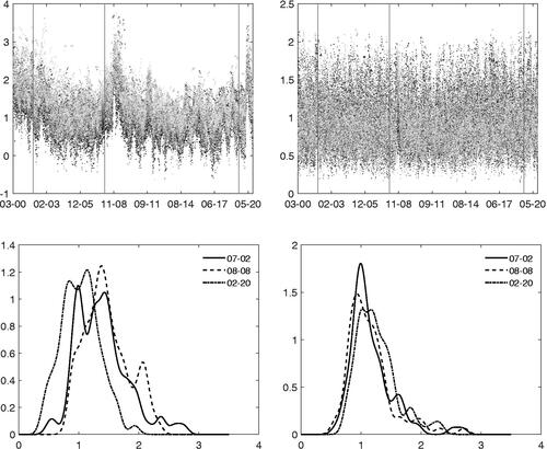
Furthermore, the cross-sectional distribution of the volatility and kurtosis exhibits multiple modes and long tails (see bottom panel). This fact seems to imply cross-section heterogeneity in the data with possible similarities in the dynamics. Given that these effects can only be partially captured by independent MS models, several multivariate GARCH models have been proposed to account for dependence (see Virbickaite, Ausín, and Galeano 2015; Bauwens and Otranto 2016, 2020).

Nevertheless, the estimation of a large number of parameters with the available data dimension may lead to intractability, overfitting and loss of efficiency. Strong restrictions, such as the parameter pooling assumption, can be used, even though those appear to be too restrictive. Instead, different approaches, such as shrinkage or sparse estimation, can be applied. Compared to standard approaches (e.g., see regularization techniques), the Bayesian framework based on hierarchical prior distributions provides a coherent approach to inference that naturally allows for partial pooling and sharing of information across equations. Bayesian inference and hierarchical priors have been successfully used in econometrics to avoid overparameterization and overfitting (e.g., see Canova and Ciccarelli 2004). Bayesian inference accommodates for various degrees of shrinking and for sparse estimation through the choice of suitable classes of prior distributions, such as Bayesian Lasso prior (Park and Casella 2008) and spike-and-slab (George and McCulloch 1993), and can be combined with other dimensionalityreduction strategies.

In this respect, evidence of cluster-wise dependence in the distribution of financial asset returns (see Bauwens and Rombouts 2007) has prompted researchers to adopt cross-sectional clustering of the time series as a building block for a dimensionality reduction step in large dimensional problems and over-parameterized models (e.g., see Hirano 2002; Billio, Casarin, and Rossini 2019; Fisher and Jensen 2022). To address this issue, this article uses a panel MSGARCH model with cross-sectional clustering based on a Bayesian nonparametric (BNP) prior (Lo 1984). In order to detect the number of regimes, we extend the approach of Otranto and Gallo (2002) to a panelframework.

A hierarchical Pitman-Yor process prior (Pitman and Yor 1997) for the MSGARCH parameters is considered. In the first stage of the hierarchical prior, cross-unit heterogeneity is allowed for, while shrinking all unit-specific parameters toward a common mean. The second stage of the hierarchy allows for mixed effects in the common mean. There are many advantages in using this hierarchical nonparametric prior. First, our approach allows for making inference on the number of mixture components in the cross-sectional clustering. Second, it adds flexibility to the model allowing for different shapes of the prior and posterior predictive distributions. Third, the predictive distribution incorporates uncertainty in the parameters and in the number of mixture components. Nonparametric Bayesian techniques have been largely and successfully used in different fields such as biostatistics (Do, Müller, and Tang 2005), biology Arbel, Mengersen, and Rousseau (2016), medicine (Xu et al. 2016), and neuroimaging (Zhang et al. 2016). For an introduction to Bayesian nonparametrics see Hjort et al. (2010) and for a review of models and applications in different fields see Müller and Mitra (2013).

The inference proposed in this article is novel in some respects. As such, the article contributes to the Bayesian nonparametrics literature for time series analysis (e.g., see Taddy and Kottas 2009; Jensen and Maheu 2010; Griffin and Steel 2011; Di Lucca et al. 2013; Bassetti, Casarin, and Leisen 2014; Billio, Casarin, and Rossini 2019; Nieto-Barajas and Quintana 2016; Griffin and Kalli 2018). The article innovates on the Bayesian nonparametric dynamic panel model in Hirano (2002) by introducing Markov-switching and GARCH dynamics and extends the nonparametric switching regression in Taddy and Kottas (2009) to a panel model with GARCH dynamics. Our approach differs from those in Hirano (2002) and Taddy and Kottas (2009), and is in line with the strategies for large dimensional and over-parameterized models (e.g., see MacLehose and Dunson 2010; Wang 2010; Billio, Casarin, and Rossini 2019), where nonparametric hierarchical priors are used to combine partial pooling and clustering effects in theparameter space.

Further, differently from Hirano (2002) and Taddy and Kottas (2009), the article uses a MCMC algorithm for posterior approximation that relies on the efficient sampling method developed in Walker (2007), Kalli, Griffin, and Walker (2011), and Hatjispyros, Nicoleris, and Walker (2011). Lastly, the article makes a contribution to the literature on Bayesian Markov-switching panel models (e.g., see Kaufmann 2010, 2015; Billio et al. 2016; Casarin et al. 2019) by introducing GARCH effects and allowing for a flexible nonparametric specification.

The estimation of MSGARCH models is also a difficult task given the path dependence problem (Gray 1996) and approximation methods have been considered (e.g., see Haas, Mittnik, and Paolella 2004; Ardia 2008; Bauwens, Preminger, and Rombouts 2010; He and Maheu 2010; Bauwens, Dufays, and Rombouts 2014; Dufays 2016; Wee, Chen, and Dunsmuir 2022). In this article, we extend the univariate Gibbs sampler by Billio, Casarin, and Osuntuyi (2016) to a multiple time series set-up and provide an efficient MCMC procedure for the hidden states of a panel MSGARCH model. The proposed method relies on a combination of blocking Gibbs and generalized Metropolis samplers.

An empirical application to financial returns of the S&P100 constituents in the United States over the period 6th January 2000–3rd October 2020 is provided. The analysis offers an optimal portfolio comparison based on one-step ahead forecasts generated by the Bayesian nonparametric panel MSGARCH (BNP-MSGARCH) and competitive models, such as a Bayesian nonparametric GARCH model without regime changes (BNP-GARCH), and a parametric GARCH. First, we detect the number of regimes using a new developed panel version of the univariate procedure by Otranto and Gallo (2002), fit the BNP-MSGARCH to the data, and examine the clusters’ composition. For the BNP-MSGARCH model, we consider two different regime identifications: (a) a restriction on the expected returns (BNP-MSGARCH-$\mu$); and (b) a restriction on the unconditional volatility level (BNP-MSGARCH-$\gamma$), for example, see Ardia et al. (2019). Second, the BNP-MSGARCH is evaluated against the other GARCH models in out-of-sample forecasts through statistical accuracy measures. Third, a portfolio exercise is carried out to ascertain economic gains. The main results show that the BNP-MSGARCH model is competitive against the other models for point-forecast and superior for density-forecast and portfolio performance.

The article is organized as follows. Section 2 describes the panel MSGARCH model and the Bayesian nonparametric prior distribution. Section 3 presents the data augmentation strategy and the posterior approximation method. Section 4 offers the empirical application. Section 5 concludes.

2 A Bayesian Nonparametric MSGARCH Model

We assume that the observable variable $y_{it}$ for the ith unit of the panel at time t satisfies (1) $$\begin{array}{cc}{y}_{it}\hfill & ={\mu }_i(s_{it})+{\sigma }_{it}{\epsilon }_{it},\hspace{1em}{\epsilon }_{it}\stackrel{\text{iid}}{\sim }\mathcal{N}(0,1),\hfill \end{array}$$(1) $$\hspace{1em}t=1,\dots ,T, i=1,\dots ,N,$$

where $\mathcal{N}(\mu ,{\sigma }^2)$ denotes the Gaussian distribution with location $\mu$ and scale $\sigma$. The conditional variance is as follows (2) $$\begin{array}{cc}{\sigma }_{it}^2\hfill & ={\gamma }_i(s_{it})+{\alpha }_i(s_{it}){\epsilon }_{it-1}^2+{\beta }_i(s_{it}){\sigma }_{it-1}^2,\hfill \end{array}$$(2) which is the MSGARCH model, and $s_{it}$, $t=1,\dots ,T$ is a hidden Markov chain process with transition probability $P(s_{it}=k|s_{it-1}=l)=p_{i,lk}$, $k,l=1,\dots ,K$, with K the number of states. The functional form for the switching parameters is (3) $$\begin{array}{cc}{\mu }_i(s_{it})\hfill & =\sum _{k=1}^K{\mu }_{ik}\mathbb{I}(s_{it}=k),\hspace{1em}{\alpha }_i(s_{it})=\sum _{k=1}^K{\alpha }_{ik}\mathbb{I}(s_{it}=k),\hfill \end{array}$$(3) (4) $${\beta }_i(s_{it})=\sum _{k=1}^K{\beta }_{ik}\mathbb{I}(s_{it}=k),\hspace{1em}{\gamma }_i(s_{it})=\sum _{k=1}^K{\gamma }_{ik}\mathbb{I}(s_{it}=k).$$(4)

We cope with the high dimension of the parameter space and related overfitting issues by exploiting cross-sectional clustering of the series. More specifically we propose to combine two modeling strategies. First, we assume soft parameter pooling through a hierarchical prior distribution with two stages, and second we introduce clustering effects in the parameter space through a nonparametric prior. The resulting joint prior distribution for the MSGARCH parameters is given by the following.

In the first stage, the rows ${\mathbf{p}}_{i,k}=(p_{i,k1},\dots ,p_{i,kK})$ of the transition matrix follow a Dirichlet distribution (5) $$(p_{i,k1},\dots ,p_{i,kK})\stackrel{\text{iid}}{\sim }\mathcal{D}ir(\varphi r_{k1},\dots ,\varphi r_{kK}),\hspace{1em}i=1,\dots ,N,$$(5) for all regimes $k=1,\dots ,K$, where the precision parameter $\varphi$ shrinks the unit-specific probabilities toward a common value ${\mathbf{r}}_k=(r_{k1},\dots ,r_{kK})$, that is the Dirichlet distribution parameter. For the second stage we assume (6) $$(r_{k1},\dots ,r_{kK})\stackrel{\text{iid}}{\sim }\mathcal{D}ir(1/K,\dots ,1/K).$$(6)

To address the high-dimensionality issue, the first stage of the hierarchical prior shrinks the switching parameters toward some common values, and the second stage clusters the units in $M_k$ groups $C_{1,k},\dots ,C_{M_k,k}$ within each regime, such that $C_{h,k}\cap C_{l,k}=\varnothing$ for $h\ne l$ and ${\cup }_{h=1}^{M_k}{C}_{h,k}=\{1,\dots ,N\}$. In the first stage, for $k=1,\dots ,K$ we assume (7) $$\begin{array}{cc}{\mu }_{ik}\hfill & \sim \mathcal{N}({\tilde{\mu }}_{ik}^{*},s),\hspace{1em}{\gamma }_{ik}/a\sim \mathcal{B}e(r{\tilde{\gamma }}_{ik}^{*}/a,r(1-{\tilde{\gamma }}_{ik}^{*}/a)),\hfill \end{array}$$(7) (8) $${\alpha }_{ik}\sim \mathcal{B}e(r{\tilde{\alpha }}_{ik}^{*},r(1-{\tilde{\alpha }}_{ik}^{*})),\hspace{1em}{\beta }_{ik}\sim \mathcal{B}e(r{\tilde{\beta }}_{ik}^{*},r(1-{\tilde{\beta }}_{ik}^{*})),$$(8) where $\mathcal{B}e(\alpha ,\beta )$ is the beta distribution with mean $\alpha /(\alpha +\beta )$ and $a>0$. The scale hyperparameters s and r are shrinking ${\theta }_{ik}=({\mu }_{ik},{\gamma }_{ik},{\alpha }_{ik},{\beta }_{ik})\in \mathbb{R}\times [0,a]\times {[0,1]}^2$ toward the parameter ${\tilde{\theta }}_{ik}^{*}=({\tilde{\mu }}_{ik}^{*},{\tilde{\gamma }}_{ik}^{*},{\tilde{\alpha }}_{ik}^{*},{\tilde{\beta }}_{ik}^{*})\in \mathbb{R}\times [0,a]\times {[0,1]}^2$ which is assumed to be constant for all units in the same cluster, that is for all $i\in C_{h,k}$ where $h=1,\dots ,M_k$ (for further details see Section 3 and (23)).

The second stage of the hierarchy generates the clusters of parameters. For each regime k we assume a Pitman-Yor process (PYP) prior (9) $$\begin{array}{cc}{\tilde{\theta }}_{ik}^{*}|G_k\stackrel{\text{iid}}{\sim }{G}_k,\hspace{1em}{G}_k\hfill & \sim \text{PYP}(\nu ,\psi ,H_0),\hfill \end{array}$$(9) with base measure $H_0$ and concentration and dispersion parameters $\nu \in [0,1]$ and $\psi >-\nu$, respectively. We assume $H_0$ is the product of independent normal and uniform distributions $\mathcal{N}(\mu ;m^{*},s^{*})$, $\mathcal{U}(\gamma ;0,a)$, $\mathcal{U}(\alpha ;0,1)$ and $\mathcal{U}(\beta ;0,1)$, which are usually chosen priors in parametric Bayesian inference for MSGARCH (e.g., see Billio, Casarin, and Osuntuyi 2016). The PYP introduced in Pitman and Yor (1997) is a generalization of the Dirichlet process which can be obtained for $\nu =0$ (e.g., see Bassetti, Casarin, and Leisen 2014).

Through the illustration of the Chinese Restaurant metaphor, the clustering structure of the PYP is defined by a Polya-Urn sampling scheme. The parameter ${\tilde{\theta }}_i^{*}$ of the ith unit is either equal to one of the other units or a new one from the base distribution $H_0$, that is, (10) $${\tilde{\theta }}_{ik}^{*}|{\tilde{\theta }}_{1k}^{*},\dots ,{\tilde{\theta }}_{i-1k}^{*}=\frac{1}{\psi -\nu +i}\sum _{j=1}^{i-1}{\delta }_{{\tilde{\theta }}_{jk}^{*}}({\tilde{\theta }}_{ik}^{*})+\frac{\psi }{\psi -\nu +i}{H}_0({\tilde{\theta }}_{ik}^{*}).$$(10)

This sequential allocation procedure generates clusters in the parameter space, where the number of clusters $M_k$ is random with the following prior distribution $$P(M_k=h)=\frac{{\nu }^{h-1}\Gamma (\psi /\nu +h)\Gamma (\psi +1)}{\Gamma (\psi /\nu +1)\Gamma (\psi +N)}{S}_{\nu }(N,h),$$with $h\in \mathbb{N}$, where $S_{\nu }(N,h)$ is a generalized Stirling number of the first kind, and $\Gamma (x)$ is the one-parameter gamma function (e.g., see Bassetti, Casarin, and Leisen 2014). To evaluate the prior mean of the number of clusters, we use $$\mathbb{E}(M_k)=\{\begin{array}{cc}\sum _{h=1}^N\frac{\psi }{\psi +h-1},\hfill & \text{if} \nu =0,\hfill \\ \frac{\Gamma (\psi +\nu +N)\Gamma (\psi +1)}{\nu \Gamma (\psi +\nu )\Gamma (\psi +N)}-\frac{\psi }{\nu },\hfill & \text{if} \nu \ne 0.\hfill \end{array}$$

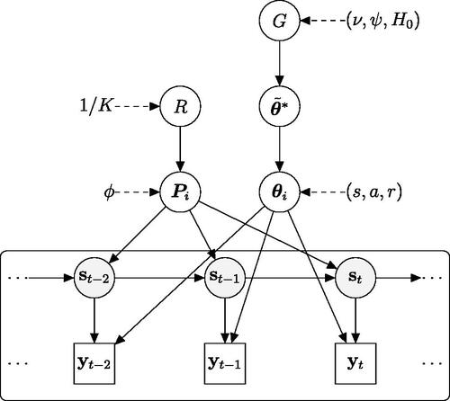
We summarize our Bayesian nonparametric model in the Directed Acyclic Graph (DAG) representation of Figure 2.

Figure 2: DAG of the Bayesian nonparametric panel MSGARCH model. It exhibits the hierarchical structure of the observations ${\mathbf{y}}_t=(y_{1t},\dots ,y_{Nt})$ (boxes), the latent state variables ${\mathbf{s}}_t=(s_{1t},\dots ,s_{Nt})$ (gray circles), the parameters of the transition probability matrix $P_i=({\mathbf{p}}_{i,1},\dots ,{\mathbf{p}}_{i,K})$, ${\theta }_i=({\mu }_i,{\gamma }_i,{\alpha }_i,{\beta }_i)$, the hyperparameters of the first stage $R=({\mathbf{r}}_1,\dots ,{\mathbf{r}}_K)$, ${\tilde{\theta }}_i^{\ast }=({\tilde{\mu }}_i^{*},{\tilde{\gamma }}_i^{*},{\tilde{\alpha }}_i^{*},{\tilde{\beta }}_i^{*})$ and of the second stage G (white circles). The directed arrows show the conditional independence structure of the model.

The PYP clustering effects on the cross section correspond to a probabilistic clustering of the parameters based on an infinite mixture distribution. The PYP can be written in a Sethuraman’s like representation as a discrete random measure (see Sethuraman 1994) (11) $$G_k(d{\theta }^{\ast })=\sum _{h=1}^{\infty }{W}_{hk}{\delta }_{{\theta }_{hk}^{\ast }}(d{\theta }^{\ast }),$$(11)

where the atoms ${\theta }_{hk}^{*}$ are iid random variables from the base measure $H_0$ and the random weights $W_{hk}$ have the stick-breaking representation (12) $$W_{hk}=V_{hk}\prod _{l=1}^{h-1}(1-V_{lk}),$$(12) with $V_{lk}\sim \mathcal{B}e(1-\nu ,\psi +\nu l)$, $l=1,2,\dots ,h$ (see Arbel, Blasi, and Prünster 2019).

By integrating out the discrete part of the hierarchical prior, the following infinite mixture representation of the prior distribution on $\theta$ is obtained (13) $$\begin{array}{cc}{\theta }_{ik}|G_k\hfill & \stackrel{\text{ind}}{\sim }\int \pi ({\theta }_{ik}|{\theta }^{*})G_k(d{\theta }^{*})=\sum _{h=1}^{\infty }{W}_{hk}\pi ({\theta }_{ik}|{\theta }_{hk}^{*}),\hfill \end{array}$$(13) where $\pi ({\theta }_{ik}|{\theta }^{*})$ is the joint parameter distribution at the first stage of hierarchical prior (see (7)–(8)) and $G_k({\theta }^{*})$ is the distribution at the second stage. In conclusion the PYP prior allows for probabilistic clustering in the parameter space.

The predictive density induced by our prior assumptions can be written as (14) $$\begin{array}{cc}{y}_{it}|G,s_{it}\hfill & \stackrel{\text{ind}}{\sim }\sum _{h=1}^{\infty }{W}_{h{s}_{it}}\int f_t(y_{it}|s_{it},{\theta }_{i{s}_{it}})\pi (d{\theta }_{i{s}_{it}}|{\theta }_{h{s}_{it}}^{*}),\hfill \end{array}$$(14) where $G=(G_1,\dots ,G_K)$ is the collection of state-dependent measures, $f_t(y_{it}|s_{it}=k,{\theta }_{i{s}_{it}})=f(y_{it}|{\mu }_{ik},{\sigma }_{ik,t})$ is the transition kernel of the MSGARCH with ${\sigma }_{ik,t}^2={\gamma }_{ik}+{\alpha }_{ik}{\epsilon }_{it-1}^2+{\beta }_{ik}{\sigma }_{it-1}^2$ for $k=1,\dots ,K$ and ${\theta }_{ik}=({\mu }_{ik},{\gamma }_{ik},{\alpha }_{ik},{\beta }_{ik})$. This prior predictive density accounts for various forms of possible heterogeneity in the data such as asymmetry, excess of kurtosis and multimodality.

3 Posterior Approximation

In this section we discuss the approximation of the posterior distribution, some identification issues and the selection of the number of regimes. We also summarize the simulation results for approximation efficiency and inference effectiveness. Let $\Theta =({\theta }_1,\dots ,{\theta }_K)$ be the collection of the units and regime parameters ${\theta }_k=({\theta }_{1k},\dots ,{\theta }_{Nk})$ and $P=(P_1,\dots ,P_N)$ the collection of transition probability matrices. Let $Y=({\mathbf{y}}_1,\dots ,{\mathbf{y}}_T)$ and $S=({\mathbf{s}}_1,\dots ,{\mathbf{s}}_T)$ be the collection over time of observation vectors ${\mathbf{y}}_t=(y_{1t},\dots ,y_{Nt})$ and of latent vectors ${\mathbf{s}}_t=(s_{1t},\dots ,s_{Nt})$, respectively. The likelihood function of the panel MSGARCH model is not tractable being written in integral form. However, a data-augmentation principle can be applied to develop efficient posterior simulation methods (Frühwirth-Schnatter 1994). We introduce the set of auxiliary allocation variables ${\xi }_{ik,t}=\mathbb{I}(s_{it}=k)$ to write the complete-data likelihood function as follows (15) $$L(Y,\Xi |\Theta ,P)=\prod _{t=1}^T\prod _{i=1}^{N}f(y_{it}|s_{it},{\theta }_{i,s_{it}})\prod _{l=1}^K\prod _{k=1}^l{p}_{i,lk}^{{\xi }_{il,t-1}{\xi }_{ik,t}},$$(15) where $\Xi =({\Xi }_1,\dots ,{\Xi }_T)$ is the collection of the latent vectors ${\Xi }_t=({\xi }_{1t},\dots ,{\xi }_{Nt})$ over time, with ${\xi }_{it}=({\xi }_{i1,t},\dots ,{\xi }_{iK,t})$.

The joint hierarchical prior distribution is (16) $$\pi (\Theta ,G)=\prod _{l=1}^K\left(\prod _{i=1}^N\pi ({\theta }_{il}|G_l)\prod _{k=1}^l{p}_{i,lk}^{r_k-1}\right)\pi (V_l)\pi ({\Theta }_l^{*}),$$(16) where the infinite mixture priors, for $k=1,\dots ,K$, are given by (17) $$\pi ({\theta }_{ik}|G_k)=\sum _{h=1}^{\infty }{W}_{hk}\pi ({\theta }_{ik}|{\theta }_{hk}^{*}),$$(17)

where $\pi ({\theta }_{ik}|{\theta }_{hk}^{*})=$ $\mathcal{N}({\mu }_{ik}|{\mu }_{hk}^{*},s)$ $\mathcal{B}e({\alpha }_{ik}|{\alpha }_{hk}^{*},r)$ $\mathcal{B}e({\beta }_{ik}|{\beta }_{hk}^{*},r)$ $\mathcal{B}e({\gamma }_{ik}/a|{\gamma }_{hk}^{*}/a,r)$ is the first-stage joint prior distribution given in (7)–(8), and (18) $$\begin{array}{cc}\pi ({\Theta }_k^{*})\hfill & =\prod _{h=1}^{\infty }\mathcal{N}({\mu }_{hk}^{*};m^{*},s^{*})\mathcal{U}({\alpha }_{hk}^{*};0,1)\mathcal{U}({\beta }_{hk}^{*};0,1)\mathcal{U}({\gamma }_{hk}^{*};0,a),\hfill \end{array}$$(18) (19) $$\pi (V_k)=\prod _{l=1}^{\infty }\mathcal{B}e(V_{lk};1-\nu ,\psi +\nu l),$$(19) are the joint distributions of the infinite collection of atoms and stick-breaking variables, ${\Theta }_k^{*}=({\theta }_{1k}^{*},{\theta }_{2k}^{*},\dots )$ and $V_k=(V_{1k},V_{2k},\dots )$, respectively.

The joint prior distribution in a Bayesian nonparametric framework is usually not tractable since its support is the space of the discrete random measures which are infinite-dimensional objects (see (17)–(19)). Nevertheless, the data-augmentation principle can be applied in order to make the inference problem more tractable. Following the recent Bayesian nonparametric literature (e.g., see Bassetti, Casarin, and Leisen 2014; Bassetti, Casarin, and Ravazzolo 2018; Billio, Casarin, and Rossini 2019), we introduce a set of slice variables $U_{ik}\sim \mathcal{U}(0,1)$ and define the index set ${\mathcal{A}}_{ik}=\left\{h\right|U_{ik}<W_{hk}\}$. Then the infinite mixture can be demarginalized as follows (20) $$\begin{array}{cc}\pi ({\theta }_{ik}|U_k,V_k,{\theta }_k^{*})\hfill & =\sum _{h=1}^{\infty }\mathbb{I}(U_{ik}<W_{hk})\pi ({\theta }_{ik}|{\theta }_{hk}^{*})\hfill \\ =\sum _{h\in {\mathcal{A}}_{ik}}\pi ({\theta }_{ik}|{\theta }_{hk}^{*}),\hfill & \hfill \end{array}$$(20) which is a almost-surely finite mixture since $\text{Card}({\mathcal{A}}_{ik})<\infty$ a.s., where $U_k=(U_{1k},\dots ,U_{Nk})$ is the collection of slice variables.

Following the standard practice in finite mixture modeling we introduce the latent allocation variable $D_{ik}\in {\mathcal{A}}_{ik}$ and obtain (21) $$\begin{array}{cc}\pi ({\theta }_{ik}|U_k,D_k,V_k,{\theta }_k^{*})\hfill & =\mathbb{I}(U_{ik}<W_{D_{ik}k})\pi ({\theta }_{ik}|{\theta }_{D_{ik}k}^{*}),\hfill \end{array}$$(21) where $D_k=(D_{1k},\dots ,D_{Nk})$. Let us denote with $V=(V_1,\dots ,V_K)$, $U=(U_1,\dots ,U_K)$ and ${\Theta }^{*}=({\theta }_1^{*},\dots ,{\theta }_K^{*})$ the collections of regime-specific auxiliary variables and atoms. The joint posterior distribution $\pi (\Xi ,\Theta ,P,U,D,V,{\Theta }^{*}|Y)$ is proportional to (22) $$\begin{array}{cc}L(Y,\Xi |\Theta ,P)\hfill & =\prod _{l=1}^K\left(\prod _{i=1}^N\pi ({\theta }_{il}|U_l,D_l,V_l,{\Theta }_l^{*})\prod _{k=1}^l{p}_{i,lk}^{r_k-1}\right)\hfill \\ \mathrm{\hspace{1em}}\mathrm{\hspace{1em}}\times \pi (V_l)\pi ({\Theta }_l).\hfill & \hfill \end{array}$$(22)

Note that the allocation variables allow to reconcile the notations used in the hierarchical model of (7) and the random measure representation in (11)–(13) as follows (23) $${\tilde{\theta }}_{ik}^{*}={\theta }_{D_{ik}k}^{*}.$$(23)

A Gibbs sampler is used to generate random samples from the joint posterior and to approximate the Bayesian estimator. The Gibbs sampler iterates the following steps

1. Sample slice and stick-breaking variables U and V given $\Xi ,\Theta ,P,D,{\Theta }^{*},Y$

2. Sample the transition probability matrices P given $\Xi ,\Theta ,U,D,V,{\Theta }^{*},Y$

3. Sample the atoms ${\Theta }^{*}$ given $\Xi ,\Theta ,P,U,D,V,Y$

4. Sample the MSGARCH parameters $\Theta$ given $\Xi ,P,U,D,V,{\Theta }^{*},Y$

5. Sample the switching allocation variables $\Xi$ given $\Theta ,P,U,D,V,{\Theta }^{*},Y$

6. Sample the mixture allocation variables D given $\Xi ,\Theta ,P,U,V,{\Theta }^{*},Y$

The derivation of the full conditional distributions and sampling method are given in Appendix A. The parameter estimator $\widehat{\theta }$, with $\theta$ element of $\Theta$, is approximated as average of MCMC draws from the posterior. The latent state estimator is approximated as ${\widehat{s}}_{it}={\sum }_{k=1}^{K}k{\widehat{\xi }}_{ik,t}$, with ${\widehat{\xi }}_{ik,t}$ the kth element of the switching allocation variable estimator ${\widehat{\xi }}_{it}=\arg \max \{\widehat{q}({\xi }_{it}|Y)\}$, where $\widehat{q}({\xi }_{it}|Y)\}$ is the MCMC approximation of the discrete posterior distribution $q({\xi }_{it}|Y)$, obtained from the Forward Filtering Backward Sampling step.

The likelihood function and the posterior distribution remain unchanged with respect to any state permutation. This identification issue and the related label switching problem are commonly solved by imposing a prior restriction on the parameters ${\theta }_{ik}$, or on a transformation $q({\theta }_{ik})$ (see Celeux 1998; Frühwirth-Schnatter 2001, 2006) such as a prior ordering, $q({\theta }_{i1})>q({\theta }_{i2})>\cdots >q({\theta }_{iK})$, with some economic interpretation. In this article we implement two alternative strategies based on performance regimes ${\mu }_{i1}>{\mu }_{i2}>\cdots >{\mu }_{iK}$ (BNP-MSGARCH-$\mu$ model) and on volatility regimes ${\gamma }_{i1}/(1-{\alpha }_{i1}-{\beta }_{i1})>{\gamma }_{i2}/(1-{\alpha }_{i2}-{\beta }_{i2})>\cdots >{\gamma }_{iK}/(1-{\alpha }_{iK}-{\beta }_{iK})$ (BNP-MSGARCH-$\gamma$ model). The first identification scheme mimics an investing strategy which classifies risky assets into different groups (styles) and move invested funds among these styles depending on their relative performance. This strategy would be decisive in monitoring the relative performance of style portfolios, especially during large market drops so to better understand where markets are heading (see Bianchi 2020). In the literature, this approach for asset allocation is known as “style investing” or “style strategies” (Barberis and Shleifer 2003) and the style identification criterion is known as “style features.” The classification of assets usually relies on industry sectors (Jame and Tong 2014) or factors (Barberis and Shleifer 2003), whereas in this article it is driven by our statistical model. The second identification scheme is more common in volatility modeling and can be used to protect portfolio allocation against excess of volatility (i.e., Barro, Canestrelli, and Consigli 2019).

In order to detect the number of regimes, we extend the univariate approach by Otranto and Gallo (2002) to a panel data framework. As in Otranto and Gallo (2002), we exploit the fact that the joint density of a panel MS model is a mixture density with the number of components equal to the number of regimes and specify the following multivariate BNP model ${\mathbf{y}}_t|({\tilde{\mu }}_t,{\tilde{\Lambda }}_t^{-1})\stackrel{\mathrm{ }\text{ind}}{\sim }{\mathcal{N}}_N({\tilde{\mu }}_t,{\tilde{\Lambda }}_t^{-1})$, $t=1,2,\dots ,T$, with location ${\tilde{\mu }}_t={({\tilde{\mu }}_{1t},\dots ,{\tilde{\mu }}_{Nt})}^{\prime }$ and diagonal precision matrix ${\tilde{\Lambda }}_t=\text{diag}({\tilde{\lambda }}_{1t},\dots ,{\tilde{\lambda }}_{Nt})$, such that $({\tilde{\mu }}_t,{\tilde{\Lambda }}_t^{-1})|G\stackrel{\text{iid}}{\sim }G$, where $G\sim \mathit{PYP}({\upsilon }_0,{\varphi }_0,G_0)$ is a PY prior. This approach is flexible and robust to structural change-points at the beginning or at the end of the sample. Procedure details are given in Appendix A. For MCMC approximation efficiency and inference effectiveness, we run simulation experiments for four different data generating processes (DGPs) using BNP-MSGARCH-$\mu$. We consider two regimes and various degrees of separation in the cluster intercept and variance. The simulation results show that the MCMC chain converges and a thinning of 10 is needed to reduce the Monte Carlo variance. Details are reported in Appendix B (supplementary materials).

4 Empirical Application

This section presents an empirical application of the BNP-MSGARCH model to the S&P100 constituents over the period 6th January 2000–3rd October 2020. 78 assets of the 101 constituents are selected in order to keep the panel balanced. Further, since style investing uses weekly or monthly predictions (e.g., see Froot and Teo 2008; Brookfield, Su, and Bangassa 2015), the percentage log-returns at weekly frequency are obtained. As a preliminary evidence, the cross-sectional heterogeneity observed in Figure 1 is robust to the choice of the rolling window size (see Appendix C, supplementary materials). In the analysis, we proceed in three steps: (i) detection of the number of regimes; (ii) forecast comparison; (iii) portfolio analysis.

The number of regimes is detected using the procedure described in Section 3, the BNP-MSGARCH model is fitted to the data (using both BNP-MSGARCH-$\mu$ and BNP-MSGARCH-$\gamma$), and the clusters’ composition is examined. We set two regimes (the extend procedure of Otranto and Gallo (2002) points to 2 regimes, see Figure C3). When ordering the expected returns in the BNP-MSGARCH-$\mu$ model (${\mu }_{i1}>{\mu }_{i2}$), regime 1 corresponds to a relative over-performance state and regime 2 to an under-performance state. Observations of the assets are assigned to one of the two regimes on the basis of the largest posterior probability (see ${\widehat{s}}_{it}$ in Section 3). We notice that this identification constraint is strongly supported by the data and allows us to separate the assets returns in two performance regimes (see Figure C4).

Figure 3: The posterior co-clustering matrix in regime 1 (left) and 2 (right) for expected returns (top) and volatility (bottom) identification constraints. In each block, gray shades represent the sector membership of the assets.

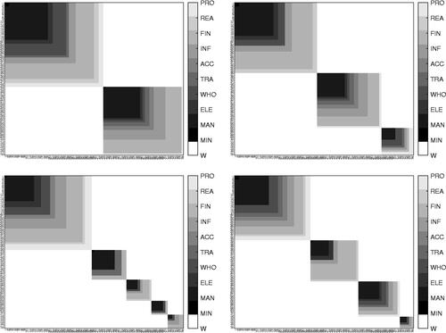
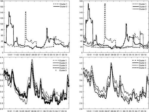
Figure 4: Price-to-Earning for the assets in clusters of regime 1 (left) and of regime 2 (right), constraint on expected returns (top panel). Logarithm of implied volatility for the assets in clusters of regime 1 (left) and of regime 2 (right), constraint on volatility (bottom panel).

For cluster identification, we assume a quite diffuse PYP prior distribution ($\nu =0$ and $\psi =10$). The posterior distribution is concentrated (see Figure C5) suggesting a substantial revision of the prior information and the MAP estimates of the number of clusters is 2 and 3 for regime 1 and 2, respectively. To study the composition of the clusters in the two regimes, we use the sector classification (for details, see Appendix C) and some fundamental financial ratios. First, we identify the clusters using the co-clustering probability matrix, which contains the probability $\mathbb{P}(\{D_{ik}=D_{jk}\left\}\right|M_k,Y)$ that the parameters ${\theta }_{ik}^{*}$ and ${\theta }_{jk}^{*}$ are in the same cluster. This probability can be easily approximated by using the MCMC samples as $\sum _{r\in {\mathcal{R}}_k}\delta (D_{jk}^{(r)}-D_{ik}^{(r)})/\text{Card}({\mathcal{R}}_k)$, where $D_{ik}^{(r)}$ is a sample of the allocation variable for the i-unit parameters in the regimes k, and ${\mathcal{R}}_k=\{r=1,\dots ,R|N_k^{(r)}=M\}$ contains the values of MCMC iterations such that the parameters of the panel units are allocated to exactly M mixture components. A spectral clustering algorithm has been applied to reorder the series and provide a better graphical representation of the clusters.

The top panel of Figure 3 reports the co-clustering matrices for the two regimes in case of expected returns identification constraint. In each block matrix, the algorithm identifies a constituent (asset) belonging to a cluster with the label 1 (gray shaded patch) and 0 (white patch) otherwise. The gray shades represent the sectors in the clusters. Following Wade and Ghahramani (2018), we use the variation of information (VI) metric proposed by Meilâ (2007) to compare the two regimes (in terms of clusters). This measure compares the information in the two regimes with the information shared between the two regimes. The normalized value of VI is equal to 0.20 (VI lies in the interval $0-{\hspace{0.17em}\log \hspace{0.17em}}_2(N)$, and a normalized value is obtained dividing VI by ${\hspace{0.17em}\log \hspace{0.17em}}_2(N)$), which suggests a substantial difference between the clustering and composition in the two regimes (see Figure 3).

In particular, for cluster 1 in both regimes, the majority of the sectors representing the assets are: manufacturing (about 40% in both regimes), financial and insurance (19% in the first regime), and wholesale and retail (25% in the second regime). Similar results for the sectors are found for cluster 2 in the two regimes: the manufacturing sector represents about 40% of the assets in the two regimes, while the financial and insurance sector is about 18% for regime 2, and information and communication is around 20%.

Further, in order to characterize the clusters in terms of the market size, measured by market capitalization, of the constituents, we first rank the companies by computing the average size of each of them using the last year of the sample period. Then, we classify the assets into three groups, namely small (bottom panel 30%), medium (middle panel 40%) and big (top panel 30%) companies (see Tab. C4). In regime 1, companies with the medium size represent the largest majority about 40%, and a similar outcome is also observed for regime 2.

For the cluster composition, we also compute the value of the Price-to-Earnings ratio (PE) for all the clusters (the average PE is computed over the last 10 years following the standard practice in style analysis). For regime 1, clusters 1 and 2 have values of PE equal to 26.97 and 32.38, respectively. For regime 2, these values are 27.08, 35.69, and 23.72 for clusters 1, 2, and 3, respectively. In both regimes cluster 2 is overvalued. Further to this, Figure 4 shows that dynamics in clusters 1 and 2 in regime 1 resemble those in regime 2.

Compared to the case of constraint on expected returns, the volatility identification strategy returns separated regimes for the single series, while the identification is less effective for the panel as a whole. Further, the posterior distribution concentrates on 5 and 4 cluster for regime 1 and 2, respectively (see Figure C5). The normalized value of VI is equal to 0.41 (see bottom panel of Figure 3). The analysis of implied volatility points to a difference in the level rather than in the dynamics (see Figure 4). Further details of all the results on cluster composition are reported in Appendix C.

As regards the one-step ahead forecast comparison, we use the following models: BNP-MSGARCH-$\mu$, BNP-MSGARCH-$\gamma$, BNP-GARCH, and GARCH. All the models are GARCH(1,1). The forecasts are computed for the period December 26, 2014–October 3, 2020 by a rolling window of 780 observations. We assess the forecasts by the RMSE and CRPS for the full out-of-sample period, and pre-COVID and COVID periods. The RMSE in Table 1 indicates that models show equal predictive ability, especially for the full out-of-sample period and the pre-COVID period, with marginal differences (Appendix C includes box-plots of RMSEs). In the COVID period, the performance of all models worsens, but the largest flexibility of the nonparametric GARCH models ensures better forecasts.

Table 1: Out-of-sample evaluation. RMSE and CRPS.

Models	RMSE
	Full period	pre-COVID period	COVID  period
BNP-MSGARCH-$\mu$	3.829	3.047	7.156
BNP-MSGARCH-$\gamma$	3.826	3.045	7.152
BNP-GARCH	3.823	3.041	7.151
GARCH	3.830	3.042	7.180
Models	CRPS
	Full period	pre-COVID period	COVID period
BNP-MSGARCH-$\mu$	1.931	1.677	3.867
BNP-MSGARCH-$\gamma$	1.927	1.674	3.865
BNP-GARCH	2.026	1.783	3.890
GARCH	2.026	1.777	3.913
Models	SR
	Full period	pre-COVID period	COVID period
BNP-MSGARCH-$\mu$	0.124	0.127	0.107
BNP-MSGARCH-$\gamma$	0.111	0.114	0.088
BNP-GARCH	0.103	0.104	0.095
GARCH	0.090	0.079	0.088

NOTES: BNP-MSGARCH-$\mu$ and BNP-MSGARCH-$\gamma$ are the Bayesian nonparametric panel Markov-Switching models with restrictions on expected returns and on volatility, respectively; GARCH is the standard GARCH model; BNP-GARCH is the Bayesian nonparametric GARCH model without regime changes. RMSE, CRPS, and SR are the averages of the root mean square error, the continuous ranked probability score, and the Sharpe ratio, respectively. The COVID period starts in early February 2020, see Centers for Disease Control and Prevention (CDC)).

When looking at CRPS, BNP-MSGARCH-$\gamma$ ranks first and BNP-MSGARCH-$\mu$ places second. This result is likely due to the fact that CRPS accounts for differences not only in mean but also in higher order moments of the forecast distributions. The BNP-GARCH and the GARCH have similar performance, with the exception of the COVID period.

A Markowitz portfolio allocation based on forecasts is carried out to establish economic gains. An investor deals with the following decision problem $V={\sum }_{i=1}^N{\sum }_{j=1}^N{X}_i{X}_j{\sigma }_{ij}$, s.t. $E={\sum }_{i=1}^N{X}_i{\mu }_{yi}=\overline{y},{\sum }_{i=1}^N{X}_i=1,X_i\ge 0$, where E is the expected return from a portfolio, $X_i$ is portfolio weights chosen to minimize the portfolio risk, and ${\mu }_{yi}$ is the expected return of the ith asset. $X_i$ is assumed to be nonnegative (no short sales). We omit the constraint $E={\sum }_{i=1}^N{X}_i{\mu }_{yi}=\overline{y}$ to build a minimum variance portfolio (see Hlouskova, Schmidheiny, and Wagner 2009). For the portfolio, we compute the Sharpe ratio for each model using the weekly treasury bill rate from Kenneth French’s data library as a risk free (RF) rate (https://mba.tuck.dartmouth.edu/pages/faculty/ken.french/data_library.html)

In terms of Sharpe ratio, BNP-MSGARCH models gain the best portfolio performance (Table 1), indicating that the largest flexibility of nonparametric models has an economic value. The portfolio proportion invested in value stocks rises in periods of increasing overperforming probability (see Figure C9). The weights to stocks with large implied volatility decrease when the probability of high-volatility regime increases. In particular, value stocks are undervalued at the beginning of the outbreak and reconvey to a larger portfolio proportion toward the end of 2020.

5 Conclusion

The study of volatility in large panels of financial assets is central for professional investors focusing on protection of invested portfolios, and for policy maker aiming at the stability of the economic system. The evidence of clusters in financial returns has attracted researchers’ attention. This article proposes a new Bayesian nonparametric (BNP) inference for Markov-switching GARCH (BNP-MSGARCH) models with clustering effects to deal with regime changes, temporal and cross-sectional clustering in large panels of financial data.

Within the BNP-MSGARCH framework, the number of regimes is detected using a new BNP procedure that extends the univariate approach of Otranto and Gallo (2002) to panel data. Further, to capture cross-sectional clustering, this article proposes a hierarchical Pitman-Yor process prior for the MSGARCH parameters. The simulations show that our posterior approximation procedure is efficient and our inference is able to recover the true value of the parameters and the number of clusters and regimes.

An application to the S&P100 constituents is offered for forecasting and portfolio allocation purposes. There is clear-cut evidence of asset clustering with heterogenous composition across sectors and style features, which ensures a superior density-forecast performance and a better portfolio allocation for the BNP-MSGARCH model.

Supplementary Materials

Simulation results and further details on the empirical application are given in the online supplementary materials.

Acknowledgments

The authors are grateful to the Editor and the Reviewers for their useful comments which significantly improved the quality of the article. Also, we would like to thank all the conference participants for helpful discussions at the “International Society for Bayesian Analysis World meeting,” 2022, Montreal, Canada, the “Annual Meeting of the Statistical Society of Canada,” 2022, Ottawa, Canada and the “Advances in Bayesian Analysis Workshop,” 2022, Venice, Italy. We benefited greatly from suggestions and discussions with Federico Bassetti, John M. Maheu, Mark J. Jensen and Herman K. van Dijk. This research used the SCSCF and HPC multiprocessor cluster systems at Ca’ Foscari University of Venice.

Appendix A

Proof of the Results in Section 3

We introduce for $h\ge 1$ the set of parameters allocated to the hth mixture component in the regime k, ${\mathcal{D}}_{hk}=\{i=1,\dots ,N|D_{ik}=h\}$ and the set of the non-empty mixture components ${\mathcal{D}}_k^{*}=\left\{h\right|{\mathcal{D}}_{hk}\ne \varnothing \}$. The number of stick-breaking components needed for the finite mixture representation is $D_k^{*}=\max \{D_{ik},i=1,\dots ,N\}$. When sampling from the full conditional distribution of ${\Theta }_k^{*}$ and $V_k$, only $N_k^{*}$ element are sampled, where $N_k^{*}$ is the smallest integer such that $\sum _{h=1}^{N_k^{*}}{W}_{hk}>1-U_k^{*}$, where $U_k^{*}=\min \{U_{ik},i=1,\dots ,N\}$.

A.1 Full Conditional Distribution of V and U

Let us split $V_k$ in three blocks: $V_k^{*}=\{V_{lk}:l\in {\mathcal{D}}_k^{*}\}$, $V_k^{**}=\{V_{k{D}_k^{*}+1},\dots ,V_{k{D}_k^{*}+N_k^{*}}\}$ and $V_k^{***}=\{V_{lk}:l>N_k^{*}\}$. The samples are generated from a collapsed Gibbs step

1. the full conditional of the elements in $V_k^{*}$ given $\Xi ,\Theta ,P,D,{\Theta }^{*},Y$ (24) $$\begin{array}{cc}f(V_{lk}|\cdots )\hfill & \propto \mathcal{B}e\mathrm{}\left(\mathrm{}1-\nu +\sum _{i=1}^N\mathbb{I}(D_{ik}=l),\psi +\nu l+\sum _{i=1}^N\mathbb{I}(D_{ik}>l)\mathrm{}\right)\hfill \\ \mathrm{\hspace{1em}}\mathrm{\hspace{1em}}\times l\le D_k^{*}\hfill & \hfill \end{array}$$(24)

2. 2. the full conditional of the elements of $V_k^{**}$ and $V_k^{***}$ given $\Xi ,\Theta ,P,D,V^{*},{\Theta }^{*},Y$, which coincides with the prior distributions $\mathcal{B}e(1-\nu ,\psi +\nu l)$ for $l>D_k^{*}$

3. the full conditional of the elements of $U_k$ given V and $\Xi ,\Theta ,P,D,{\Theta }^{*},Y$, $f(U_{ik}|\cdots )\propto \mathbb{I}(U_{ik}<W_{D_{ik}k})$, which is uniform on the interval $(0,W_{D_{ik}})$

A.2 Full Conditional Distribution of P and R

We apply a collapsed-Gibbs step and sample ${\mathbf{r}}_k$, $k=1,\dots ,K$, given $\Xi ,{\Theta }_{-p},D,V,Y$, and ${\mathbf{p}}_k=({\mathbf{p}}_{1,k},\dots ,{\mathbf{p}}_{N,k})$, $k=1,\dots ,K$, is the collection of the kth row of the transition probability matrices given $({\mathbf{r}}_1,\dots ,{\mathbf{r}}_K)$ and $\Xi ,{\Theta }_{-p},D,V,Y$. As for the transition probabilities, from standard calculations in Markov-switching regressions we obtain (25) $$\begin{array}{cc}f({\mathbf{p}}_{i,k}|\cdots )\hfill & \propto \prod _{h=1}^K{p}_{i,kh}^{\varphi r_{kh}+n_{i,kh}-1}\hfill \end{array}$$(25) $$\begin{array}{cc}\propto \hfill & \mathcal{D}ir(\varphi r_{k1}+n_{i,k1},\dots ,\varphi r_{kK}+n_{i,kK}),\hfill \end{array}$$where $n_{i,kh}={\sum }_{t=1}^T{\xi }_{\mathit{ikt}-1}{\xi }_{\mathit{iht}}$. The marginal distribution is $$\begin{array}{cc}f({\mathbf{r}}_k|\cdots )\hfill & \propto {\int }_{{\Delta }_{{[0,1]}^K}^N}\prod _{i=1}^N\prod _{h=1}^K{p}_{i,kh}^{\varphi r_{kh}+n_{i,kh}-1}\frac{\Gamma (\varphi )}{\Gamma (\varphi r_{kh})}d{p}_{i,kh}\pi ({\mathbf{r}}_k)\hfill \\ \propto \hfill & \prod _{h=1}^K{r}_{kh}^{d-1}\prod _{i=1}^N\frac{\Gamma (\varphi r_{kh}+n_{i,kh})}{\Gamma (\varphi +n_{i,k})}\frac{\Gamma (\varphi )}{\Gamma (\varphi r_{kh})},\hfill \end{array}$$

where $n_{i,k}=n_{i,k1}+\cdots +n_{i,kK}$, and ${\Delta }_{{[0,1]}^K}=\{(p_1,\dots ,p_K)\in {\mathbb{R}}^K|p_k>0 \forall k, p_1+\cdots +p_K=1\}$ is the K-dim standard simplex. From the properties of the gamma functions $$\begin{array}{cc}\Gamma (\varphi r_{kh}+n_{i,kh})\hfill & =\prod _{l=1}^{n_{i,kh}}(\varphi r_{kh}+l-1)\Gamma (\varphi r_{kh}),\hfill \\ \Gamma (\varphi +n_{i,k})=\prod _{l=1}^{n_{i,k}}(\varphi +l-1)\Gamma (\varphi ),\hfill & \hfill \end{array}$$we have: $f({\mathbf{r}}_k|\cdots )\propto \mathcal{D}ir(1/K+m_{k1},\dots ,1/K+m_{kK})g({\mathbf{r}}_k)$, where $g({\mathbf{r}}_k)={\prod }_{i=1}^N{\prod }_{h=1}^K{\prod }_{l=2}^{n_{i,kh}}(\varphi r_{kh}+l-1)$, $m_{kh}=\text{Card}({\mathcal{M}}_{kh})$ and ${\mathcal{M}}_{kh}=\{i=1,\dots ,N|n_{i,kh}>0\}$. Samples from this full conditional distribution are obtained by a Metropolis-Hastings (MH) algorithm with independent proposal distribution $\mathcal{D}ir(1/K+m_{k1},\dots ,1/K+m_{kK})$.

A.3 Full Conditional Distribution of ${\Theta }^{*}$

The full conditional distribution of ${\mathbf{\theta }}_{hk}^{*}=({\mu }_{hk}^{*},{\gamma }_{hk}^{*},{\alpha }_{hk}^{*},{\beta }_{hk}^{*})$ can be sampled by simulating iteratively from the following conditional distributions. The full conditional of ${\mu }_{hk}^{*}$ is $$\begin{array}{cc}f({\mu }_{hk}^{*}|\cdots )\hfill & \propto \mathcal{N}({\mu }_{hk}^{*}|m^{*},s^{*})\prod _{i\in {\mathcal{D}}_{hk}}\mathcal{N}({\mu }_{ik}|{\mu }_{hk}^{*},s)\hfill \\ \propto \mathcal{N}\left({\mu }_{hk}^{*}|{\overline{m}}_{hk},{\overline{s}}_{hk}\right),\hfill & \hfill \end{array}$$where ${\overline{m}}_{hk}={\overline{s}}_{hk}^2\left(\frac{m^{*}}{s^{*2}}+\frac{\sum _{i\in {\mathcal{D}}_{hk}}{\mu }_{ik}}{s^2}\right)$ and ${\overline{s}}_{hk}={(\frac{1}{s^{*2}}+\frac{\text{Card}({\mathcal{D}}_{hk})}{s^2})}^{-1/2}.$ The full conditional distribution of ${\gamma }_{hk}^{*}$ is (26) $$f({\gamma }_{hk}^{*}|\cdots )\propto {\mathbb{I}}_{[0,a]}({\gamma }_{hk}^{*})\prod _{i\in {\mathcal{D}}_{hk}}\mathcal{B}e({\gamma }_{ik}/a|r{\gamma }_{hk}^{*}/a,r(1-{\gamma }_{hk}^{*}/a)),$$(26) $$\begin{array}{c}\propto {\mathbb{I}}_{[0,a]}({\gamma }_{hk}^{*})\\ \prod _{i\in {\mathcal{D}}_{hk}}\frac{\hspace{0.17em}\exp \hspace{0.17em}\{(r{\gamma }_{hk}^{*}/a-1)\hspace{0.17em}\log \hspace{0.17em}({\gamma }_{ik}/a)+(r(1-{\gamma }_{hk}^{*}/a)-1)\hspace{0.17em}\log \hspace{0.17em}(1-{\gamma }_{ik}/a)\}}{\Gamma (r{\gamma }_{hk}^{*}/a)\Gamma (r(1-{\gamma }_{hk}^{*}/a))},\\ \propto \hspace{0.17em}\exp \hspace{0.17em}\{-{\kappa }_{hk}{\gamma }_{hk}^{*}\}{\left(\frac{1}{\Gamma (r{\gamma }_{hk}^{*}/a)\Gamma (r(1-{\gamma }_{hk}^{*}/a))}\right)}^{\text{Card}({\mathcal{D}}_{hk})}{\mathbb{I}}_{[0,a]}({\gamma }_{hk}^{*}),\end{array}$$ where ${\kappa }_{hk}=\frac{r}{a}\sum _{i\in {\mathcal{D}}_{hk}}\hspace{0.17em}\log \hspace{0.17em}((a-{\gamma }_{ik})/{\gamma }_{ik})$ samples from this conditional distribution are obtained by a MH algorithm with independent proposal distribution $(1-\hspace{0.17em}\exp \hspace{0.17em}\{-{\kappa }_{hk}{\gamma }_{hk}^{*}\}){(1-\hspace{0.17em}\exp \hspace{0.17em}\{-a{\kappa }_{hk}\})}^{-1}{\mathbb{I}}_{[0,a]}({\gamma }_{hk}^{*})$. The full conditional of ${\alpha }_{hk}^{*}$ is

$\begin{array}{c}f({\alpha }_{hk}^{*}|\cdots )\propto {\mathbb{I}}_{[0,1]}({\alpha }_{hk}^{*})\hfill \\ \hspace{1em}\prod _{i\in {\mathcal{D}}_{hk}}\frac{\hspace{0.17em}\exp \hspace{0.17em}\{(r{\alpha }_{hk}^{*}-1)\hspace{0.17em}\log \hspace{0.17em}({\alpha }_{ik})+(r(1-{\alpha }_{hk}^{*})-1)\hspace{0.17em}\log \hspace{0.17em}(1-{\alpha }_{ik})\}}{\Gamma (r{\alpha }_{hk}^{*})\Gamma (r(1-{\alpha }_{hk}^{*}))},\hfill \\ \propto \hspace{0.17em}\exp \hspace{0.17em}\{-{\tau }_{hk}{\alpha }_{hk}^{*}\}{(\frac{1}{\Gamma (r{\alpha }_{hk}^{*})\Gamma (r(1-{\alpha }_{hk}^{*}))})}^{\mathrm{ }\text{Card}({\mathcal{D}}_{hk})}{\mathbb{I}}_{[0,1]}({\alpha }_{hk}^{*}),\hfill \end{array}$ where ${\tau }_{hk}=r\sum _{i\in {\mathcal{D}}_{hk}}\hspace{0.17em}\log \hspace{0.17em}((1-{\alpha }_{ik})/{\alpha }_{ik})$. Samples from this conditional distribution are obtained by MH with independent proposal distribution $(1-\hspace{0.17em}\exp \hspace{0.17em}\{-{\tau }_{hk}{\alpha }_{hk}^{*}\}){(1-\hspace{0.17em}\exp \hspace{0.17em}\{-{\tau }_{hk}\})}^{-1}{\mathbb{I}}_{[0,1]}({\alpha }_{hk}^{*})$. Similar argument is applied to derive the full conditional distributions of ${\beta }_{hk}^{*}$.

A.4 Full Conditional Distribution of $\Theta$

The full conditional distribution of the elements of ${\theta }_{ik}$ $k=1,\dots ,K$ is discussed. Let ${\mu }_i=({\mu }_{i1},\dots ,{\mu }_{iK})$, its full conditional distribution is (27) $$f({\mu }_i|\cdots )\propto \left(\prod _{t=1}^T\mathcal{N}(y_{it}|{\mu }_i(s_{it}),{\sigma }_{it})\right)\prod _{k=1}^K\mathcal{N}({\mu }_{ik}|{\tilde{\mu }}_{ik}^{*},s),$$(27) which is not tractable due to the recursive form of ${\sigma }_{it}^2$. Thus, we sample from the full conditional by MH with proposal distribution obtained through the approximation ${\sigma }_{it}^{*2}$ of ${\sigma }_{it}^2$. The joint full conditional of ${\mu }_i$ can be approximated by a normal distribution with mean ${\mathbf{m}}_i=S_i{(m_{i1}/s_{i1}^2,m_{i2}/s_{i2}^2,\dots ,m_{iK}/s_{iK}^2)}^{\prime }$ and diagonal covariance matrix $S_i=\text{diag}(s_{i1}^2,s_{i2}^2,\dots ,s_{iK}^2)$ where $m_{ik}=s_{ik}^2\left(\frac{{\tilde{\mu }}_{ik}^{*}}{s^2}+\sum _{t\in {\mathcal{T}}_{y,ik}}\frac{y_{it}}{{\sigma }_{it}^{*2}}\right)$ and $s_{ik}^2={\left(\frac{1}{s^2}+\sum _{t\in {\mathcal{T}}_{y,ik}}\frac{1}{{\sigma }_{it}^{*2}}\right)}^{-1}$, with ${\mathcal{T}}_{y,ik}=\{t=1,\dots ,T|s_{it}=k\}$ and ${\sigma }_{it}^{*2}={\gamma }_i(s_{it})+{\alpha }_i(s_{it}){(y_{t-1}-{\mu }_i(s_{it-1}))}^2+({\beta }_i(s_{it})){\sigma }_{t-1}^{*2}.$ The constructed mean and variance are used to define the parameters of the normal mixture proposal distribution for ${\mu }_i$, that is $f({\mu }_i|\dots )=0.05\mathcal{N}({\mu }_i|{\mathbf{m}}_i,S_i)+0.95\mathcal{N}({\mu }_i|{\mu }_i^{(r-1)},S_i).$ As regards the parameters of the volatility process, the full conditional is (28) $$\begin{array}{cc}f({\gamma }_i,{\alpha }_i,{\beta }_i|\cdots )\propto \hfill & \prod _{k=1}^K\mathcal{B}e({\gamma }_{ik}/a|r{\tilde{\gamma }}_{ik}^{*}/a,r(1-{\tilde{\gamma }}_{ik}^{*}/a))\hfill \end{array}$$(28) $$\begin{array}{c}\mathcal{B}e({\alpha }_{ik}|r{\tilde{\alpha }}_{ik}^{*},r(1-{\tilde{\alpha }}_{ik}^{*}))\\ \mathcal{B}e({\beta }_{ik}|r{\tilde{\beta }}_{ik}^{*},r(1-{\tilde{\beta }}_{ik}^{*}))\prod _{t=1}^T\mathcal{N}(y_{it}|{\mu }_i(s_{it}),{\sigma }_{it}),\end{array}$$ where ${\gamma }_i=({\gamma }_{i1},\dots ,{\gamma }_{iK})$, ${\alpha }_i=({\alpha }_{i1},\dots ,{\alpha }_{iK})$ and ${\beta }_i=({\beta }_{i1},\dots ,{\beta }_{iK})$. We follow the ARMA approximation of the MSGARCH process, that is (29) $${\sigma }_{it}^2={\gamma }_i(s_{it})\mathrm{}+\mathrm{}{\alpha }_i(s_{it}){ϵ}_{it-1}^2+{\beta }_i(s_{it}){\sigma }_{it-1}^2,$$(29) (30) $$\begin{array}{c}{ϵ}_{it}^2={\gamma }_i(s_{it})+({\alpha }_i(s_{it})\mathrm{}+\mathrm{}{\beta }_i(s_{it})){ϵ}_{it-1}^2\mathrm{}-\mathrm{}{\beta }_i(s_{it})({ϵ}_{it-1}^2\mathrm{}-\mathrm{}{\sigma }_{it-1}^2)\\ \mathrm{\hspace{1em}}\mathrm{\hspace{1em}}+({ϵ}_{it}^2\mathrm{}-\mathrm{}{\sigma }_{it}^2).\end{array}$$(30)

Let $w_{it}={ϵ}_{it}^2-{\sigma }_{it}^2=\left(\frac{{ϵ}_{it}^2}{{\sigma }_{it}^2}-1\right){\sigma }_{it}^2=({\chi }^2(1)-1){\sigma }_{it}^2$ with $E_{t-1}[w_{it}]=0$ and ${\text{var}}_{t-1}[w_{it}]=2{\sigma }_{it}^4$. Subject to the above, we assume $w_{it}\approx w_{it}^{*}\sim \mathcal{N}(0,2{\sigma }_{it}^4)$ (Nakatsuma 1998). The auxiliary ARMA model for the squared error term ${ϵ}_{it}^2$ is ${ϵ}_{it}^2={\gamma }_i{s}_{it}+({\alpha }_i(s_{it})+{\beta }_i(s_{it})){ϵ}_{it-1}^2-{\beta }_i(s_{it})w_{it-1}^{*}+w_{it}^{*}$ with $w_{it}^{*}\sim \mathcal{N}(0,2{\sigma }_{it}^4)$, which returns $w_{it}^{*}={ϵ}_{it}^2-{\gamma }_i(s_{it})-{\alpha }_i(s_{it}){ϵ}_{it-1}^2-{\beta }_i(s_{it})({ϵ}_{it-1}^2-w_{it-1}^{*})$. Following Ardia (2008) we further express $w_{it}^{*}$ as a linear function of the $(3K\times 1)$ vector of volatility parameters ${\theta }_{i\sigma }={({\gamma }_{i1},\dots ,{\gamma }_{iK},{\alpha }_{i1},\dots ,{\alpha }_{iK},{\beta }_{i1},\dots ,{\beta }_{iK})}^{\prime }$. To do this, we approximate the function $w_t^{*}$ by the first order Taylor’s expansion about ${\theta }_{i\sigma }^{(r-1)}={({\gamma }_{i1}^{(r-1)},\dots ,{\gamma }_{iK}^{(r-1)},{\alpha }_{i1}^{(r-1)},\dots ,{\alpha }_{iK}^{(r-1)},{\beta }_{i1}^{(r-1)},\dots ,{\beta }_{iK}^{(r-1)})}^{\prime }$ as (31) $$w_{it}^{*}\approx w_{it}^{**}=w_{it}^{*}({\theta }_{i\sigma }^{(r-1)})+{\nabla }_{it}^{\prime }({\theta }_{i\sigma }-{\theta }_{i\sigma }^{(r-1)}),$$(31) where ${\nabla }_{it}^{\prime }=({\nabla }_{it1},{\nabla }_{it2},\dots ,{\nabla }_{\mathit{itK}})$ with ${\nabla }_{\mathit{itk}}^{\prime }=(\frac{\partial w_{it}^{*}}{\partial {\gamma }_{ik}},\frac{\partial w_{it}^{*}}{\partial {\alpha }_{ik}},\frac{\partial w_{it}^{*}}{\partial {\beta }_{ik}})$. ${\nabla }_{it}^{\prime }$ satisfies the recurrence: ${\nabla }_{it}^{\prime }={\mathbf{u}}_t^{\prime }{\xi }_{it}+{\nabla }_{it-1}^{\prime }({\beta }_i{\xi }_{it}^{\prime })$, where ${\mathbf{u}}_t=(-1,-{ϵ}_{it-1}^2,-({ϵ}_{it-1}^2-w_{it-1}^{*}))$, ${\nabla }_{i0k}=\mathcal{0}$ and ${\xi }_{it}$ is a row vector.

Upon defining $r_{it}^{*}=w_{it}^{*}({\theta }_{-i\pi }^{(r-1)})-{\nabla }_{it}^{\prime }{\theta }_{i\sigma }^{(r-1)}$, it turns out that $w_{it}^{**}=r_{it}^{*}+{\nabla }_{it}^{\prime }{\theta }_{i\sigma }$. Furthermore, by defining ${\mu }_i=({\mu }_{i1},{\mu }_{i2},\dots ,{\mu }_{iK})$,the $T\times 1$ vectors ${\mathbf{w}}_i={(w_{i1}^{**},\dots ,w_{iT}^{**})}^{\prime }$ and ${\mathbf{r}}_i^{*}={(r_{i1}^{*},\dots ,r_{iT}^{*})}^{\prime }$, and a $T\times 3K$ matrix ${\nabla }_i={({\nabla }_{i1},{\nabla }_{i2},\dots ,{\nabla }_{iT})}^{\prime }$ as well as a $T\times T$ diagonal matrix ${{\rm Y}}_i=2\text{diag}({\sigma }_{i1}^{**4},{\sigma }_{i2}^{**4},\dots ,{\sigma }_{iT}^{**4})$ with ${\sigma }_{it}^{**2}=({\xi }_{it}{\gamma }_i^{{(r-1)}^{\prime }})+({\xi }_{it}{\alpha }_i^{{(r-1)}^{\prime }}){(y_{t-1}-{\xi }_{t-1}{\mu }_i^{{(r)}^{\prime }})}^2+({\xi }_{it}{\beta }_i^{{(r-1)}^{\prime }}){\sigma }_{it-1}^{**2}$, we have ${\mathbf{w}}_i={\mathbf{r}}_i^{*}+{\nabla }_i{\theta }_{i\sigma }$. Using this linear approximation, the full conditional distribution of ${\theta }_{i\sigma }$ approximates as (32) $$\begin{array}{cc}f({\theta }_{i\sigma }|{\xi }_{i,1:T}^{(r-1)},{\mu }_i^{(r)},y_{1:T})\hfill & \propto \frac{1}{|{{\rm Y}}_i{|}^{\frac{1}{2}}}\exp \hspace{0.17em}\left(-\frac{{\mathbf{w}}_i^{\prime }{{\rm Y}}_i^{-1}{\mathbf{w}}_i}{2}\right){\mathbb{I}}_{\Theta }({\theta }_{i\sigma })\hfill \\ \propto {\mathcal{N}}_{3K}({\mathbf{m}}_{i\sigma },S_{i\sigma }){\mathbb{I}}_{\Theta }({\theta }_{i\sigma }),\hfill & \hfill \end{array}$$(32) where $\Theta =\{{\gamma }_{i1}>0,\dots ,{\gamma }_{iK}>0,0<{\alpha }_{i1}<1,\dots ,0<{\alpha }_{iK}<1,0<{\beta }_{i1}<1\dots ,0<{\beta }_{iK}<1\}$ and $S_{i\sigma }={({\nabla }_i^{\prime }{{\rm Y}}_i^{-1}{\nabla }_i)}^{-1}$, ${\mathbf{m}}_{i\sigma }=-S_{i\sigma }{\nabla }_i^{\prime }{{\rm Y}}_i^{-1}{\mathbf{r}}_i^{*}$. The mean and variance defined above are used to characterize proposal distribution for ${\theta }_{i\sigma }$, that is a mixture of truncated normal distributions. In our MCMC exercise, we sample ${\theta }_{i\sigma }$ from the normal mixture $f({\theta }_{i\sigma }|\dots )=0.05\mathcal{N}({\theta }_{i\sigma }|{\mathbf{m}}_{i\sigma },S_{i\sigma })+0.95\mathcal{N}({\theta }_{i\sigma }|{\theta }_{i\sigma }^{(r-1)},S_{i\sigma })$ and check that each sample satisfies the constraints.

A.5 Full Conditional Distribution of $\Xi$

The full joint conditional distribution of the state variables, ${\xi }_{i,1:T}=({\xi }_{i1},\dots ,{\xi }_{iT})$ with ${\xi }_{it}=({\xi }_{i1,t},\dots ,{\xi }_{iK,t})$, given the parameter values and return series (33) $$p({\xi }_{i,1:T}|\dots )\propto \prod _{t=1}^{T}f(y_{it}|s_{it},{\theta }_{i{s}_{it}},)\prod _{k=1}^K\prod _{l=1}^k{p}_{i,lk}^{{\xi }_{\mathit{ilt}-1}{\xi }_{\mathit{ikt}}},$$(33) is a nonstandard distribution. For this reason, following Billio, Casarin, and Osuntuyi (2016), we propose a MH algorithm with proposal distribution given by an approximation of the smoothed probability $p({\xi }_{i,1:T}|\dots )$. The algorithm involves running a Forward Filtering Backward Sampling (FFBS) on an auxiliary model to generate proposals at each iteration step (Carter and Kohn 1994; Frühwirth-Schnatter 1994). Among several alternative collapsing procedures (see Billio, Casarin, and Osuntuyi 2016), we adopt the MSGARCH model by Klaassen (2002) as an auxiliary model as it accounts for the highest amount of information in its construction. We denote the proposal distribution by (34) $$q({\xi }_{i,1:T}|{\theta }_i,y_{i,1:T})=q({\xi }_{iT}|{\theta }_i,y_{i,1:T})\prod _{t=1}^{T-1}q({\xi }_{it}|{\xi }_{it+1},{\theta }_i,y_{i,1:t}),$$(34)

where $q({\xi }_{it}|{\xi }_{it+1},{\theta }_i,y_{i,1:t})=q({\xi }_{it}|y_{i,1:t},{\theta }_i)q({\xi }_{it+1}|{\xi }_{it},{\theta }_i)/q({\xi }_{it+1}|$ $y_{i,1:t},{\theta }_i)$, and $q({\xi }_{it}|y_{i,1:t},{\theta }_i)$ is the filtered probability. At time t, given ${\theta }_i$ and $y_{i,1:t}$, the predicted and filtered distributions are (35) $$\begin{array}{cc}q({\xi }_{it}|{\theta }_i,y_{i,1:t-1})\hfill & =\sum _{k=1}^K\left(\prod _{l=1}^K{p}_{i,lk}^{{\xi }_{il,t}}\right)q({\xi }_{it-1}={\mathcal{e}}_k|{\theta }_i,y_{i,1:t-1}),\hfill \end{array}$$(35) (36) $$\begin{array}{cc}q({\xi }_{it}|{\theta }_i,y_{i,1:t})\hfill & =g(y_{it}|{\xi }_{it},{\theta }_i,y_{i,1:t-1})q({\xi }_{it}|{\theta }_i,y_{i,1:t-1})/c,\hfill \end{array}$$(36) where $c={\sum }_{k=1}^{K}g(y_{it}|{\xi }_{it}={\mathbf{e}}_k,{\theta }_i,y_{i,1:t-1})q({\xi }_{it}={\mathbf{e}}_k|{\theta }_i,y_{i,1:t-1})$, ${\mathbf{e}}_k$ is the $k-$ th row of the identity matrix $I_K$. The conditional density of the unit i under the auxiliary model is (37) $$g(y_{it}|{\xi }_{it},{\theta }_i,y_{i,1:t-1})\propto \prod _{\tau =1}^t\frac{1}{h_{i\tau }}\hspace{0.17em}\exp \hspace{0.17em}\left(-\frac{{(y_{i\tau }-{\mu }_i(s_{i\tau }))}^2}{2h_{i\tau }^2}\right),$$(37) where $h_{it}^2={\gamma }_i(s_{it})+{\alpha }_i(s_{it}){ϵ}_{(y)it-1}^2+{\beta }_i(s_{it}){\sigma }_{(y)i,kt-1}^2$ with ${ϵ}_{(y)it-1}=y_{it-1}-{\mu }_{(y)i,kt-1}$, ${\mu }_{(y)ik,t-1}=E[{\mu }_i(s_{it})|y_{i,1:t-1},{\xi }_{it}={\mathbf{e}}_k]$, and ${\sigma }_{(y)i,kt-1}^2=E[{\sigma }_{it-1}^2(y_{i,1:t-2},{\xi }_{it-1},{\xi }_{it-2})|y_{i,1:t-1},{\xi }_{it}={\mathbf{e}}_k]$.

Using the output of the forward filtering, we compute $q({\xi }_{iT}|{\theta }_i,y_{i,1:T})$ and $q({\xi }_{it}|{\xi }_{it+1},{\theta }_i,y_{i,1:t})\propto {\prod }_{l=1}^K{({\sum }_{k=1}^K{p}_{i,lk}{\xi }_{i1,t})}^{{\xi }_{il,t+1}}q({\xi }_{it}|{\theta }_i,y_{i,1:t})$, $t=T-1,T-2,\dots ,2,1$. Then, at each time, step we sample ${\xi }_T$ from $q({\xi }_T|{\theta }_i,y_{i,1:T})$ and ${\xi }_{it}$ from $q({\xi }_{it}|{\xi }_{it+1},{\theta }_i,y_{i,1:t})$ iteratively for $t=T-1,T-2,\dots ,2,1$. This is the backward sampling step. Samples from $q({\xi }_{it}|{\xi }_{it+1},{\theta }_i,y_{i,1:t})$ can be obtained by multinomial sampling.

A.6 Full Conditional Distribution of D

The full conditional of $D_{ik}$ is $P(D_{ik}=h|\cdots )=c_h/c$ for $h\in {\mathcal{A}}_{ki}$, with $c_h=\mathcal{N}({\mu }_{ik}|{\mu }_{hk}^{*},s)$ $\mathcal{B}e({\alpha }_{ik}|r{\alpha }_{hk}^{*},r(1-{\alpha }_{hk}^{*}))$ $\mathcal{B}e({\beta }_{ik}|r{\beta }_{hk}^{*},r(1-{\beta }_{hk}^{*}))\mathcal{B}e({\gamma }_{ik}/a|r{\gamma }_{hk}^{*}/a,r(1-{\gamma }_{hk}^{*}/a))/a$ where $c=\sum _{h\in {\mathcal{A}}_{ki}}{c}_h$ is the normalizing constant and a a real positive constant.

A.7 Detection of the Number of Regimes

We present the panel version of the univariate approach by Otranto and Gallo (2002). We assume ${\mathbf{y}}_t|$ $({\tilde{\mu }}_t,$ ${\tilde{\Lambda }}_t^{-1})$ $\stackrel{\text{ind}}{\sim }$ ${\mathcal{N}}_N($ ${\tilde{\mu }}_t,$ ${\tilde{\Lambda }}_t^{-1})$, $t=1,$ 2,…, T, with $({\tilde{\mu }}_t,$ ${\tilde{\Lambda }}_t^{-1})$ $|G\stackrel{\text{iid}}{\sim }G$, and $G\sim$ $\mathit{PYP}({\upsilon }_0,$ ${\varphi }_0,G_0)$. The BNP model allows for the infinite mixture representation ${\mathbf{y}}_t|$ $G\sim$ ${\sum }_{k=1}^{\infty }{W}_k$ $\phi ({\mathbf{y}}_t|$ ${\mu }_k,$ ${\Lambda }_k^{-1})$, where $\phi (\mathbf{y}|\mu ,\Sigma )$ denotes the density of a multivariate normal with location and scale parameters, $\mu$ and $\Sigma$, respectively. We assume the base measure $G_0$ is a product of N independent hierarchical prior distributions $G_0(\mu ,\Lambda )=$ $\mathcal{G}a(\tau ;c/2,d/2)$ ${\prod }_{j=1}^N$ $\mathcal{N}({\mu }_j;m_j,\tau {\lambda }_j^{-1})$ $\mathcal{G}a({\lambda }_j;a/2,b/2)$. Instead of using the sampler in Otranto and Gallo (2002), we apply a more efficient sampler which relies on the stick-breaking representation (Walker 2007). The sampler requires the use of the allocation, $D_t\stackrel{\text{iid}}{\sim }P(D_t=k)=W_k$ $t=1,\dots ,T$, stick-breaking $V_k\stackrel{\text{ind}}{\sim }\mathcal{B}e(1-{\upsilon }_0,{\varphi }_0+k{\upsilon }_0)$ $k=1,2,\dots ,$ and slice $U_t\sim \mathcal{U}(0,W_{D_t})$ variables. The allocation variable has the interpretation of regime allocation as in Otranto and Gallo (2002). The full conditionals of ${\mu }_k$, ${\Lambda }_k$, and $\tau$ are (38) $$\begin{array}{cc}f({\mu }_{kj}|\cdots )\hfill & \propto \mathcal{N}((\sum _{t\in {\mathcal{D}}_k}{y}_{jt}+m_j\tau )/((T_k+\tau )),1/({\lambda }_{kj}(T_k+\tau ))),\hfill \end{array}$$(38) (39) $$\begin{array}{c}f({\lambda }_{kj}|\cdots )\propto \mathcal{G}a((T_k+a)/2,((T_k-1)s_{jk}^2+(T_k\tau {(m_j-{\overline{y}}_{jk})}^2)/\\ (T_k+\tau )+b)/2),\end{array}$$(39) (40) $$\begin{array}{cc}f(\tau |\cdots )\hfill & \propto \mathcal{G}a((N+c)/2,(d+\sum _{j=1}^N{({\mu }_{kj}-m_j)}^2{\lambda }_{kj})/2),\hfill \end{array}$$(40)

$j=1,\dots ,N$, where ${\mathcal{D}}_k=\{t=1,\dots ,T|D_t=k\}$, $T_k=\text{Card}({\mathcal{D}}_k)$ $s_{jk}^2=\sum _{t\in {\mathcal{D}}_k}{(y_{jt}-{\overline{y}}_{jk})}^2/(T_k-1)$, ${\overline{y}}_{jk}=\sum _{t\in {\mathcal{D}}_k}{y}_{jt}/T_k$. Let $D^{*}=\max \{D_t,t=1,\dots ,T\}$ be the maximum value of the allocation variables, and $D_t^{*}$ the smallest integer such that $\sum _{k=1}^{D_t^{*}}{W}_k>1-U_t$. Since $D_t^{*}<\infty$ a.s., the infinite mixture reduces to a finite mixture. The full conditionals of the steak-breaking components, the slice variables and the allocation variables are (41) $$\begin{array}{cc}f(V_l|\cdots )\hfill & \propto \mathcal{B}e(1-{\upsilon }_0+\sum _{t=1}^T\mathbb{I}(D_t=l),{\varphi }_0+{\upsilon }_{0}l\hfill \end{array}$$(41) (42) $$\begin{array}{c}\mathrm{\hspace{1em}}\mathrm{\hspace{1em}}+\sum _{t=1}^T\mathbb{I}(D_{ik}>l)), l\le D^{*},\\ f(U_t|\cdots )\propto \mathcal{U}(U_t<W_{D_t}),\end{array}$$(42) (43) $$\begin{array}{cc}f(D_t=k|\cdots )\hfill & \propto \phi ({\mathbf{y}}_t|{\mu }_k,{\Lambda }_k^{-1}), k\le D_t^{*}.\hfill \end{array}$$(43)

References

- Ang, A., and Timmermann, A. (2012), “Regime Changes and Financial Markets,” Annual Review of Financial Economics, 4, 313–337. DOI: 10.1146/annurev-financial-110311-101808.
- Arbel, J., Blasi, P. D., and Prünster, I. (2019), “Stochastic Approximations to the Pitman–Yor Process,” Bayesian Analysis, 14, 1201–1219. DOI: 10.1214/18-BA1127.
- Arbel, J., Mengersen, K., and Rousseau, J. (2016), “Bayesian Nonparametric Dependent Model for Partially Replicated Data: The Influence of Fuel Spills on Species Diversity,” The Annals of Applied Statistics, 10, 1496–1516. DOI: 10.1214/16-AOAS944.
- Ardia, D. (2008), Financial Risk Management with Bayesian Estimation of GARCH Models: Theory and Applications, volume 612 of Lecture Notes in Economics and Mathematical Systems, Berlin: Springer.
- Ardia, D., Bluteau, K., Boudt, K., Catania, L., and Trottier, D.-A. (2019), “Markov-Switching GARCH Models in R: The MSGARCH Package,” Journal of Statistical Software, 91, 1–38. DOI: 10.18637/jss.v091.i04.
- Barberis, N., and Shleifer, A. (2003), “Style Investing,” Journal of Financial Economics, 68, 161–199. DOI: 10.1016/S0304-405X(03)00064-3.
- Barro, D., Canestrelli, E., and Consigli, G. (2019), “Volatility versus Downside Risk: Performance Protection in Dynamic Portfolio Strategies,” Computational Management Science, 16, 433–479. DOI: 10.1007/s10287-018-0310-4.
- Bassetti, F., Casarin, R., and Leisen, F. (2014), “Beta-Product Dependent Pitman-Yor Processes for Bayesian Inference,” Journal of Econometrics, 180, 49–72. DOI: 10.1016/j.jeconom.2014.01.007.
- Bassetti, F., Casarin, R., and Ravazzolo, F. (2018), “Bayesian Nonparametric Calibration and Combination of Predictive Distributions,” Journal of the American Statistical Association, 113, 675–685. DOI: 10.1080/01621459.2016.1273117.
- Bauwens, L., Dufays, A., and Rombouts, J. (2014), “Marginal Likelihood for Markov-switching and Change-Point GARCH,” Journal of Econometrics, 178, 508–522. DOI: 10.1016/j.jeconom.2013.08.017.
- Bauwens, L., and Otranto, E. (2016), “Modeling the Dependence of Conditional Correlations on Market Volatility,” Journal of Business and Economic Statistics, 34, 254–268. DOI: 10.1080/07350015.2015.1037882.
- Bauwens, L., and Otranto, E. (2020), “Nonlinearities and Regimes in Conditional Correlations with Different Dynamics,” Journal of Econometrics, 217, 496–522.
- Bauwens, L., Preminger, A., and Rombouts, J. (2010), “Theory and Inference for a Markov Switching GARCH Model,” Econometrics Journal, 13, 218–244. DOI: 10.1111/j.1368-423X.2009.00307.x.
- Bauwens, L., and Rombouts, J. (2007), “Bayesian Clustering of Many GARCH Models,” Econometric Reviews, 26, 365–86. DOI: 10.1080/07474930701220576.
- Bianchi, F. (2020), “The Great Depression and the Great Recession: A View from Financial Markets,” Journal of Monetary Economics, 114, 240–261. DOI: 10.1016/j.jmoneco.2019.03.010.
- Billio, M., Casarin, R., and Osuntuyi, A. (2016), “Efficient Gibbs Sampling for Markov Switching GARCH Models,” Computational Statistics and Data Analysis, 100, 37–57. DOI: 10.1016/j.csda.2014.04.011.
- Billio, M., Casarin, R., Ravazzolo, F., and Van Dijk, H. (2016), “Interactions between Eurozone and US Booms and Busts: A Bayesian Panel Markov-switching VAR Model,” Journal of Applied Econometrics, 31, 1352–1370. DOI: 10.1002/jae.2501.
- Billio, M., Casarin, R., and Rossini, L. (2019), “Bayesian Nonparametric Sparse VAR Models,” Journal of Econometrics, 212, 97–115. DOI: 10.1016/j.jeconom.2019.04.022.
- Bollerslev, T. (1986), “Generalized Autoregressive Conditional Heteroskedasticity,” Journal of Econometrics, 31, 307–327. DOI: 10.1016/0304-4076(86)90063-1.
- Brookfield, D., Su, C., and Bangassa, K. (2015), “Investment Style Positioning of UK Unit Trusts,” The European Journal of Finance, 21, 946–970. DOI: 10.1080/1351847X.2013.788533.
- Canova, F., and Ciccarelli, M. (2004), “Forecasting and Turning Point Prediction in a Bayesian Panel VAR Model,” Journal of Econometrics, 120, 327–359. DOI: 10.1016/S0304-4076(03)00216-1.
- Carter, C. K., and Kohn, R. (1994), “On Gibbs Sampling for State Space Models,” Biometrika, 81, 209–230. DOI: 10.1093/biomet/81.3.541.
- Casarin, R., Foroni, C., Marcellino, M., and Ravazzolo, F. (2019), “Uncertainty Through the Lenses of a Mixed-Frequency Bayesian Panel Markov Switching Model,” Annals of Applied Statistics, 12, 2559–2586.
- Celeux, G. (1998), “Bayesian Inference for Mixture: The Label Switching Problem,” in Compstat, eds. R. Payne and P. Green, pp. 227–232, Heidelberg: Physica.
- Di Lucca, M., Guglielmi, A., Müller, P., and Quintana, F. (2013), “A Simple Class of Bayesian Nonparametric Autoregression Models,” Bayesian Analysis, 8, 63–88. DOI: 10.1214/13-BA803.
- Do, K.-A., Müller, P., and Tang, F. (2005), “A Bayesian Mixture Model for Differential Gene Expression,” Journal of the Royal Statistical Society, Series C, 54, 627–644. DOI: 10.1111/j.1467-9876.2005.05593.x.
- Dufays, A. (2016), “Infinite-state Markov-switching for Dynamic Volatility and Correlation Models,” Journal of Financial Econometrics, 14, 418–460. DOI: 10.1093/jjfinec/nbv017.
- Engle, R. F. (1982), “Autoregressive Conditional Heteroscedasticity with Estimates of the Variance of United Kingdom Inflation,” Econometrica, 50, 987–1007. DOI: 10.2307/1912773.
- Fisher, M., and Jensen, M. J. (2022), “Bayesian Nonparametric Learning of How Skill is Distributed Across the Mutual Fund Industry,” Journal of Econometrics, 230, 131–153. DOI: 10.1016/j.jeconom.2021.04.002.
- Froot, K., and Teo, M. (2008), “Style Investing and Institutional Investors,” Journal of Financial and Quantitative Analysis, 43, 883–906. DOI: 10.1017/S0022109000014381.
- Frühwirth-Schnatter, S. (1994), “Data Augmentation and Dynamic Linear Models,” Journal of Time Series Analysis, 15, 183–202. DOI: 10.1111/j.1467-9892.1994.tb00184.x.
- Frühwirth-Schnatter, S.(2001), “Markov Chain Monte Carlo Estimation of Classical and Dynamic Switching and Mixture Models,” Journal of the American Statistical Association, 96, 194–209.
- Frühwirth-Schnatter, S.(2006), Finite Mixture and Markov Switching Models, New York: Springer.
- George, E. I., and McCulloch, R. E. (1993), “Variable Selection via Gibbs Sampling,” Journal of the American Statistical Association, 88, 881–889. DOI: 10.1080/01621459.1993.10476353.
- Gray, S. F. (1996), “Modeling the Conditional Distribution of Interest Rates as a Regime-switching Process,” Journal of Financial Economics, 42, 27–62. DOI: 10.1016/0304-405X(96)00875-6.
- Griffin, J., and Kalli, M. (2018), “Bayesian Nonparametric Vector Autoregressive Models,” Journal of Econometrics, 203, 267–282. DOI: 10.1016/j.jeconom.2017.11.009.
- Griffin, J. E., and Steel, M. F. J. (2011), “Stick-Breaking Autoregressive Processes,” Journal of Econometrics, 162, 383–396. DOI: 10.1016/j.jeconom.2011.03.001.
- Haas, M., Mittnik, S., and Paolella, M. (2004), “A New Approach to Markov Switching GARCH Models,” Journal of Financial Econometrics, 2, 493–530. DOI: 10.1093/jjfinec/nbh020.
- Hatjispyros, S. J., Nicoleris, T. N., and Walker, S. G. (2011), “Dependent Mixtures of Dirichlet Processes,” Computational Statistics & Data Analysis, 55, 2011–2025. DOI: 10.1016/j.csda.2010.12.005.
- He, Z., and Maheu, J. (2010), “Real Time Detection of Structural Breaks in GARCH Models,” Computational Statistics & Data Analysis, 54, 2628–2640. DOI: 10.1016/j.csda.2009.09.038.
- Hirano, K. (2002), “Semiparametric Bayesian Inference in Autoregressive Panel Data Models,” Econometrica, 70, 781–799. DOI: 10.1111/1468-0262.00305.
- Hjort, N. L., Homes, C., Müuller, P., and Walker, S. G. (2010), Bayesian Nonparametrics, Cambridge: Cambridge University Press.
- Hlouskova, J., Schmidheiny, K., and Wagner, M. (2009), “Multistep Predictions for Multivariate GARCH Models: Closed form Solution and the Value for Portfolio Management,” Journal of Empirical Finance, 14, 330–336. DOI: 10.1016/j.jempfin.2008.09.002.
- Jame, R., and Tong, Q. (2014), “Industry-based Style Investing,” Journal of Financial Markets, 19, 110–130. DOI: 10.1016/j.finmar.2013.08.004.
- Jensen, J. M., and Maheu, M. J. (2010), “Bayesian Semiparametric Stochastic Volatility Modeling,” Journal of Econometrics, 157, 306–316. DOI: 10.1016/j.jeconom.2010.01.014.
- Kalli, M., Griffin, J. E., and Walker, S. G. (2011), “Slice Sampling Mixture Models,” Statistics and Computing, 21, 93–105. DOI: 10.1007/s11222-009-9150-y.
- Kaufmann, S. (2010), “Dating and Forecasting Turning Points by Bayesian Clustering with Dynamic Structure: A Suggestion with an Application to Austrian Data,” Journal of Applied Econometrics, 25, 309–344. DOI: 10.1002/jae.1076.
- Kaufmann, S. (2015), “K-state Switching Models with Time-varying Transition Distributions: Does Loan Growth Signal Stronger Effects of Variables on Inflation?” Journal of Econometrics, 187, 82–94.
- Klaassen, F. (2002), “Improving GARCH Volatility Forecasts with Regime Switching GARCH,” Empirical Economics, 27, 363–394. DOI: 10.1007/s001810100100.
- Lo, A. Y. (1984), “On a Class of Bayesian Nonparametric Estimates: I. Density Estimates,” The Annals of Statistics, 12, 351–357. DOI: 10.1214/aos/1176346412.
- MacLehose, R., and Dunson, D. (2010), “Bayesian Semiparametric Multiple Shrinkage,” Biometrics, 66, 455–462. DOI: 10.1111/j.1541-0420.2009.01275.x.
- Meilâ, M. (2007), “Comparing Clusterings – An Information Based Distance,” Journal of Multivariate Analysis, 98, 873–895.
- Müller, P., and Mitra, R. (2013), “Bayesian Nonparametric Inference – Why and How,” Bayesian Analysis, 8, 269–302. DOI: 10.1214/13-BA811.
- Nakatsuma, T. (1998), “A Markov-chain Sampling Algorithm for GARCH Models,” Studies in Nonlinear Dynamics and Econometrics, 3, 107–117.
- Nieto-Barajas, L. E., and Quintana, F. A. (2016), “A Bayesian Non-parametric Dynamic AR Model for Multiple Time Series Analysis,” Journal of Time Series Analysis, 37, 675–689. DOI: 10.1111/jtsa.12182.
- Otranto, E., and Gallo, G. M. (2002), “A Nonparametric Bayesian Approach to Detect the Number of Regimes in Markov Switching Models,” Econometric Reviews, 21, 477–496. DOI: 10.1081/ETC-120015387.
- Park, T., and Casella, G. (2008), “The Bayesian Lasso,” Journal of the American Statistical Association, 103, 681–686. DOI: 10.1198/016214508000000337.
- Pitman, J., and Yor, M. (1997), “The Two Parameter Poisson-Dirichlet Distribution Derived from a Stable Subordinator,” Annals of Probability, 25, 855–900.
- Sethuraman, J. (1994), “A Constructive Definition of Dirichlet Priors,” Statistica Sinica, 4, 639–650.
- Taddy, M. A., and Kottas, A. (2009), “Markov Switching Dirichlet Process Mixture Regression,” Bayesian Analysis, 4, 793–816. DOI: 10.1214/09-BA430.
- Virbickaite, A., Ausín, M. C., and Galeano, P. (2015), “Bayesian Inference Methods for Univariate and Multivariate GARCH Models: A Survey,” Journal of Economic Surveys, 29, 76–96. DOI: 10.1111/joes.12046.
- Wade, S., and Ghahramani, Z. (2018), “Bayesian Cluster Analysis: Point Estimation and Credible Balls,” (with discussion), Bayesian Analysis, 13, 559–626. DOI: 10.1214/17-BA1073.
- Walker, S. G. (2007), “Sampling the Dirichlet Mixture Model with Slices,” Communications in Statistics - Simulation and Computation, 36, 45–54. DOI: 10.1080/03610910601096262.
- Wang, H. (2010), “Sparse Seemingly Unrelated Regression Modelling: Applications in Finance and Econometrics,” Computational Statistics & Data Analysis, 54, 2866–2877. DOI: 10.1016/j.csda.2010.03.028.
- Wee, D. C., Chen, F., and Dunsmuir, W. T. (2022), “Likelihood Inference for Markov Switching GARCH(1,1) Models using Sequential Monte Carlo,” Econometrics and Statistics, 21, 50–68. DOI: 10.1016/j.ecosta.2020.03.004.
- Xu, Y., Müller, P., Wahed, A. S., and Thall, P. F. (2016), “Bayesian Nonparametric Estimation for Dynamic Treatment Regimes with Sequential Transition Times,” Journal of the American Statistical Association, 111, 921–950. DOI: 10.1080/01621459.2015.1086353.
- Zhang, L., Guindani, M., Versace, F., Engelmann, J. M., and Vannucci, M. (2016), “A Spatiotemporal Nonparametric Bayesian Model of Multi-subject fMRI Data,” The Annals of Applied Statistics, 10, 638–666. DOI: 10.1214/16-AOAS926.