A General Framework for Constructing Locally Self-Normalized Multiple-Change-Point Tests

Abstract

We propose a general framework to construct self-normalized multiple-change-point tests with time series data. The only building block is a user-specified single-change-detecting statistic, which covers a large class of popular methods, including the cumulative sum process, outlier-robust rank statistics, and order statistics. The proposed test statistic does not require robust and consistent estimation of nuisance parameters, selection of bandwidth parameters, nor pre-specification of the number of change points. The finite-sample performance shows that the proposed test is size-accurate, robust against misspecification of the alternative hypothesis, and more powerful than existing methods. Case studies of the Shanghai-Hong Kong Stock Connect turnover are provided.

KEYWORDS:

• Nonparametric
• Recursive computation
• Time series
• Tuning-free

1 Introduction

Testing structural stability is critical in statistical inference. There is a considerable amount of literature and practical interest in testing for the existence of change points. Csörgö and Horváth (1988, 1997) provided comprehensive solutions to the at-most-one-change (AMOC) problem using both classical parametric and nonparametric approaches. One method assumes a fixed number of change points (m) for the multiple-change-point problem. The test statistics are constructed by dividing the data into segments and maximizing a sum of AMOC statistics computed within each segment; see Antoch and Jarušková (2013) and Shao and Zhang (2010). However, such approaches are vulnerable to misspecification of the true number of change points M and the computational cost often increases exponentially with m. Another method uses sequential estimation (Vostrikova 1981; Bai and Perron 1998). This class of methods sequentially performs AMOC tests and produces estimates if the no-change-point hypothesis is rejected. Because the structural difference of data before and after a particular change point may be less apparent in the presence of other change points, the AMOC-type tests may lose their power under the multiple-change-point setting.

Localization can be used to improve power. Bauer and Hackl (1980) introduced the moving sum approach. Chu, Hornik, and Kaun (1995) and Eichinger and Kirch (2018) later applied the approach to change-point detection. This method selects a fixed window size and performs inference on each subsample. Fryzlewicz (2014) proposed wild binary segmentation, which draws subsamples without fixing the window size, to avoid window size selection. Both algorithms attempt to find a subsample containing only one change point to boost power without specifying m. If the standard CUSUM process is used, the methods require consistent and change-point-robust estimation of the long-run variance, which can be nontrivial and may require tuning a bandwidth parameter (Andrews 1991). Worse still, different bandwidths can noticeably influence the tests (Kiefer and Vogelsang 2005). To avoid the challenging estimation, Lobato (2001) first proposed using a self-normalizer that converges to a pivotal distribution proportional to the nuisance parameter. Shao and Zhang (2010) later applied self-normalization to the AMOC problem. In the multiple-change-point problem, Zhang and Lavitas (2018) proposed a self-normalized test that intuitively scans for the first and last change points. However, it may compromise power when larger changes occur in the middle.

In this article, our contributions are as follows: (a) We propose a novel localized self-normalization framework to transform AMOC statistics into powerful and size-accurate multiple-change-point tests, which apply to a broad class of time series models and a large class of AMOC statistics, including the CUSUM process and outlier-robust change-detecting statistics, instead of any specific process as constructed in existing methods. (b) The methods support multiple-change-point detection in general model parameters. The resulting tests achieve promising power. (c) Our test is also shown to be locally powerful asymptotically. (d) The novel self-normalizers can be recursively computed. (e) The test allows an intuitive extension to estimation with good theoretical properties.

The rest of the article is structured as follows. Section 2 reviews the self-normalization method proposed by Shao and Zhang (2010) under the AMOC problem. Section 3.1 presents the proposed framework, and of Sections 3.2–3.4 explore applications of some popular change-detecting processes and extensions to estimation. In Section 4, the differences between various self-normalized approaches are comprehensively discussed. Some implementation issues are also discussed. Simulation results are presented in Section 5, which show good size accuracy and a substantial improvement in power. The article ends with a real-data analysis of the Shanghai-Hong Kong Stock Connect turnover in Section 6. Proofs of the main results are presented in the Appendix. A supplement containing additional simulation results, recursive formulas, algorithms, and an extension to long-range dependent time series is also included. An R-package “SNmct” is available online.

2 Introduction of Self-Normalization

Consider the signal-plus-noise model: $X_i={\mu }_i+Z_i$, where ${\mu }_i=\mathsf{E}(X_i)$ for $i=1,\dots ,n$ and $\{Z_i:i\in \mathbb{Z}\}$ is a stationary noise sequence. The AMOC testing problem is formulated as follows: (2.1) $$H_0:{\mu }_1=\cdots ={\mu }_n,$$(2.1) (2.2) $$H_1:\exists 1<k_1<n,\hspace{1em}{\mu }_1=\cdots ={\mu }_{k_1}\ne {\mu }_{k_1+1}=\cdots ={\mu }_n.$$(2.2)

Let ${\xi }_{k_1,k_2}={\sum }_{i=k_1}^{k_2}{X}_i$ if $1\le k_1\le k_2\le n$; ${\xi }_{k_1,k_2}=0$ otherwise. A popular statistic for detecting a single change point is the CUSUM process, defined as (2.3) $${\text{C}}_n(\lfloor nt\rfloor )=n^{-1/2}\sum _{i=1}^{\lfloor nt\rfloor }\left(X_i-n^{-1}{\xi }_{1,n}\right),$$(2.3) where $t\in [0,1]$ and $\lfloor nt\rfloor$ is the largest integer part of nt. The limiting distribution of the functional in (2.3) is established by the following assumption.

Assumption 2.1.

As $n\to \infty ,\{n^{-1/2}{\sum }_{i=1}^{\lfloor nt\rfloor }{Z}_i:t\in [0,1]\}\Rightarrow \{\sigma \mathbb{B}(t):t\in [0,1]\},$ where ${\sigma }^2=\underset{n\to \infty }{\text{lim}}\text{var}({\xi }_{1,n})/n\in (0,\infty )$ is the long-run variance, $\mathbb{B}(·)$ is the standard Brownian motion and “$\Rightarrow$” denotes convergence in distribution in the Skorokhod space (Billingsley 1999).

Assumption 2.1 is known as the functional central limit theorem or Donsker’s invariance principle. Under standard regularity conditions, Assumption 2.1 is satisfied. For example, Herrndorf (1984) proved the functional central limit theorem for the dependent data under some mixing conditions; Wu (2007) later proved the strong convergence for stationary processes using physical and predictive dependence measures. Under the null hypothesis H₀, by the continuous mapping theorem, we have $\{{\text{C}}_n(\lfloor nt\rfloor ):t\in [0,1]\}\Rightarrow \{\sigma \left\{\mathbb{B}(t)-t\mathbb{B}(1)\right\}:t\in [0,1]\}$.

Classically, the celebrated Kolmogorov–Smirnov test statistic, defined as ${\text{KS}}_n(\sigma )=\underset{k=1,\dots ,n}{\text{sup}}|{\text{C}}_n(k)/\sigma |$, can be used for the AMOC problem. Because σ is typically unknown, we estimate it by an estimator $\widehat{\sigma }$ that is consistent under H₀ and H₁; see Chan (2022a, 2022b) for some possible estimators. Hence, ${\text{KS}}_n(\widehat{\sigma })$ converges to $\underset{t\in (0,1)}{\text{sup}}|\mathbb{B}(t)-t\mathbb{B}(1)|$, which is known as the Kolmogorov distribution. Shao and Zhang (2010) proposed to bypass the estimation of σ by normalizing ${\text{C}}_n(k)$ by a nondegenerate standardizing random process called a self-normalizer: $$\begin{array}{c}{\text{V}}_n(k)=n^{-2}\{\sum _{i=1}^k{\left({\xi }_{1,i}-\frac{i}{k}{\xi }_{1,k}\right)}^2\\ \mathrm{\hspace{1em}}\mathrm{\hspace{1em}}+\sum _{i=k+1}^n{\left({\xi }_{i,n}-\frac{n-i+1}{n-k}{\xi }_{k+1,n}\right)}^2\},\end{array}$$where $k=1,\dots ,n-1$. The resulting self-normalized test statistic for the AMOC problem is ${\text{S}}_n^{(1)}$, where (2.4) $$\begin{array}{c}{\text{S}}_n^{(1)}=\underset{k=1,\dots ,n-1}{\text{sup}}{\text{S}}_n^{(1)}(k)\mathrm{\hspace{1em}}\mathrm{\hspace{1em}}\text{and}\\ {\text{S}}_n^{(1)}(k)={\text{C}}_n^2(k)/{\text{V}}_n(k).\end{array}$$(2.4)

Under Assumption 2.1 and H₀, the limiting distribution of ${\text{S}}_n^{(1)}$ is nondegenerate and pivotal. The nuisance parameter ${\sigma }^2$ is asymptotically cancelled out in the numerator ${\text{C}}_n^2(k)$ and the denominator ${\text{V}}_n(k)$ on the right-hand side of (2.4). Moreover, because there is no change point in the intervals $[1,k_1]$ and $[k_1+1,n]$ under H₁, the self-normalizer at the true change point, ${\text{V}}_n(k_1)$, is invariant to the change, and therefore their proposed test does not suffer from the well-known non-monotonic power problem; see, for example, Vogelsang (1999).

However, this appealing feature no longer exists in the multiple-change-point setting. Moreover, their proposed self-normalizer is specifically designed for normalizing the CUSUM process, which may not be the best choice if the data have a heavy-tailed distribution. In the next section, we propose a framework for extending user-specified AMOC statistics to a multiple-change-point self-normalized test using the localization idea.

3 General Framework

3.1 Locally Self-Normalized Test Statistic

We consider the multiple-change-point testing problem, that is, to test the H₀ in (2.1) against (3.1) $$\begin{array}{c}{H}_{\ge 1}:{\mu }_1=\cdots ={\mu }_{k_1}\ne {\mu }_{k_1+1}=\cdots ={\mu }_{k_2}\ne \cdots \ne {\mu }_{k_M+1}\\ =\cdots ={\mu }_n,\end{array}$$(3.1) for unknown times $1<k_1<\cdots <k_M<n$, and an unknown number of change points $M\ge 1$. In this section, combining the advantages of localization and self-normalization, we lay out the underlying principles to define a general class of statistics for testing the existence of multiple change points.

Generally, for the AMOC problem, one may consider any specific global change-detecting process, ${\{{\text{D}}_n(\lfloor nt\rfloor )\}}_{0\le t\le 1}$. For some positive definite matrix ${\sigma }_{\text{D}}$ and some empirical process $\mathbb{D}(·)$ with a pivotal distribution, ${\{{\text{D}}_n(\lfloor nt\rfloor )\}}_{0\le t\le 1}$ converges weakly to ${\sigma }_{\text{D}}\mathbb{D}(·)$ in the Skorokhod space. Typically, ${\text{D}}_n(k)$ is designed to detect whether k is a change point for $k=1,\dots ,n$. We generalize the input global change-detecting process into a localized change-detecting statistic, defined as (3.2) $$\begin{array}{c}{\text{L}}_n^{(\text{D})}(k|s,e)={\left(\frac{n}{e-s+1}\right)}^{1/2}[{\text{D}}_n(k)-{\text{D}}_n(s-1)\\ \mathrm{\hspace{1em}}\mathrm{\hspace{1em}}-\frac{k-s+1}{e-s+1}\left\{{\text{D}}_n(e)-{\text{D}}_n(s-1)\right\}],\end{array}$$(3.2) where $1\le s\le k\le e\le n$. By the continuous mapping theorem, ${\text{L}}_n^{(\text{D})}(·|s,e)$ converges in distribution to a random variable proportional to a nuisance parameter σ_D. A self-normalizer is constructed by a function of the global change-detecting process to cancel σ_D, defined as (3.3) $$\begin{array}{c}{\text{V}}_n^{(\text{D})}(k|s,e)=\frac{k-s+1}{{(e-s+1)}^2}\sum _{j=s}^k{\text{L}}_n^{(\text{D})}{(j|s,k)}^{\otimes 2}\\ \mathrm{\hspace{1em}}\mathrm{\hspace{1em}}+\frac{e-k}{{(e-s+1)}^2}\sum _{j=k+1}^e{\text{L}}_n^{(\text{D})}{(j|k+1,e)}^{\otimes 2},\end{array}$$(3.3) where $A^{\otimes 2}=A{A}^{\text{T}}$ for any matrix A. For $1\le s\le k\le e\le n$, define (3.4) $${\text{T}}_n^{(\text{D})}(k|s,e)={\text{L}}_n^{(\text{D})}{(k|s,e)}^{\text{T}}{\text{V}}_n^{(\text{D})}{(k|s,e)}^{-1}{\text{L}}_n^{(\text{D})}(k|s,e),$$(3.4) and set ${\text{T}}_n^{(\text{D})}(k|s,e)=0$ otherwise. By the continuous mapping theorem, it is not difficult to see that ${\text{T}}_n^{(\text{D})}(·|·)$ is asymptotically pivotal. Consequently, ${\text{T}}_n^{(\text{D})}(k|s,e)$ is a generalized locally self-normalized (LSN) statistic for detecting whether k is a change point over the local window $[s,e]$. To infer whether k is a change point, we aggregate ${\text{T}}_n^{(\text{D})}(k|·)$ over all of the symmetric local windows and propose the score function, defined as (3.5) $${\text{T}}_n^{(\text{D})}(k)=\underset{\lfloor nϵ\rfloor \le d\le n}{\text{sup}}{\text{T}}_n^{(\text{D})}(k|k-d,k+1+d),$$(3.5) where $0<ϵ<1/2$ is a fixed local tuning parameter, which is similarly used in, for example, Huang, Volgushev, and Shao (2015) and Zhang and Lavitas (2018); see Remark 3.1 for the rationale for considering only the symmetric local windows. In particular, they suggested choosing $ϵ=0.1$, which is used throughout this article. Essentially, (3.5) compares the local subsamples of length d + 1 before and after time k, that is, ${\mathcal{S}}_{\text{before}}=\{X_{k-d},\dots ,X_k\}$ and ${\mathcal{S}}_{\text{after}}=\{X_{k+1},\dots ,X_{k+1+d}\}$, for each possible width d that is not too small. The statistic ${\text{T}}_n^{(\text{D})}(k)$ records the change corresponding to the most discernible d; see Section 3.2 for more discussion on the change-detecting ability of the LSN statistic. Finally, to capture the effects of all potential change points, we aggregate the scores ${\text{T}}_n^{(\text{D})}(k)$ across k and obtain the proposed test statistic, (3.6) $${\text{T}}_n^{(\text{D})}=\frac{1}{n-2\lfloor ϵn\rfloor -1}\sum _{k=\lfloor ϵn\rfloor +1}^{n-\lfloor ϵn\rfloor -1}{\text{T}}_n^{(\text{D})}(k).$$(3.6)

Our framework constructs multiple-change-point tests through a two-layer aggregation process. The first aggregation across d is to let the data choose the window sizes. We remark that the performance of the moving sum (MOSUM) statistic, which is a special case of the localized CUSUM with a fixed window size, depends critically on the window size (Eichinger and Kirch 2018). To handle window size selection, Cho and Kirch (2022) proposed localized pruning by first taking the union of fixed bandwidth change-point estimators produced by the MOSUM method or other multiscale method over a specific grid of bandwidths, and then pruning down the size of the first-step estimator. Although the procedure may work for point estimation, it is unclear whether it can be extended to construct powerful tests. The proposed framework employs an automatic window selection, based on the strength of discrepancy of ${\mathcal{S}}_{\text{before}}$ and ${\mathcal{S}}_{\text{after}}$ according to the LSN statistic, prior to the estimation stage to avoid additional pruning. Nevertheless, both authors suggested considering multiple bandwidths for robustness.

The purpose of the second layer is to gather all information on all possible change points. Generally, users may choose their preferred aggregation operators, for example, median, trimmed mean, etc, for aggregation. Formally, for any finite set of indices $S\subset \mathbb{Z}$ having a size $\left|S\right|$, we say that $\mathcal{P}$ is an aggregation operator if ${\mathcal{P}}_{i\in S}{a}_i$ maps $\{a_i\in \mathbb{R}:i\in S\}$ to a real number. For example, if $\mathcal{P}=\text{max},{\mathcal{P}}_{i\in S}{a}_i={\text{max}}_{i\in S}{a}_i$ gives the maximum; and if $\mathcal{P}=\text{mean},{\mathcal{P}}_{i\in S}{a}_i=\sum _{i\in S}{a}_i/\left|S\right|$ gives the sample mean. Hence, the most general form of our proposed test statistic is $$\begin{array}{c}{\text{T}}_n^{(\text{D})}={\text{T}}_n^{(\text{D})}[{\mathcal{P}}^{(1)},{\mathcal{P}}^{(2)}]\\ ={\mathcal{P}}_{\lfloor ϵn\rfloor <k<n-\lfloor ϵn\rfloor }^{(2)}\left[{\mathcal{P}}_{\lfloor nϵ\rfloor \le d\le n}^{(1)}\left\{{\text{T}}_n^{(\text{D})}(k|k-d,k+1+d)\right\}\right],\end{array}$$where ${\mathcal{P}}^{(1)}$ and ${\mathcal{P}}^{(2)}$ are some aggregation operators. The optimal choices of aggregation operators depend on the number of change points and their respective sizes. By construction, the scores (3.5) remain large over the neighborhoods of the true change points. Intuitively, the average score captures evidence from all change points and their neighborhoods, whereas the maximum score can only capture evidence from a single change point corresponding to the highest score. According to our experience and the simulation results provided in Section C.12 of the supplement, the gain in power is noticeable when ${\mathcal{P}}^{(2)}=\text{mean}$ and all the changes are of the same size. However, the gain diminishes as the portions of smaller changes increase relative to those of larger changes. Nevertheless, ${\text{T}}_n^{(\text{D})}[\text{max},\text{mean}]$ still has greater power in the cases considered. Therefore, we recommend selecting ${\mathcal{P}}^{(2)}=\text{mean}$, as used in the rest of this article.

Our approach is more flexible as it supports a general change-detecting process ${\text{D}}_n(·)$ and general aggregation operators ${\mathcal{P}}^{(1)}$ and ${\mathcal{P}}^{(2)}$. Moreover, the locally self-normalized statistic is a function of the supplied global change-detecting process. Therefore, recursive computation of the locally self-normalized statistics, regardless of the input change-detecting process, is possible for our approach. Briefly, our framework is an automatic procedure for generalizing any single-change-detecting statistic ${\text{D}}_n(·)$ to a multiple-change-detecting statistic ${\text{T}}_n^{(\text{D})}$. We demonstrate this feature through various examples. Section 3.2 presents the theoretical details of the proposed framework under the popular CUSUM process. An application of outlier robust statistic is demonstrated in Section 3.3. Extension to testing change in general parameters is discussed in Section 3.4.

Remark 3.1

(Symmetric windows). Let the score function based on nonsymmetric windows be ${\tilde{\text{T}}}_n^{(\text{D})}(k)=\underset{\lfloor ϵn\rfloor \le d_0,d_1\le n}{\text{sup}}{\text{T}}_n^{(\text{D})}$ $(k|k-d_0,k+1+d_1)$. The corresponding test statistic is ${\tilde{\text{T}}}_n^{(\text{D})}={\sum }_{k=\lfloor ϵn\rfloor +1}^{n-\lfloor ϵn\rfloor -1}{\tilde{\text{T}}}_n^{(\text{D})}(k)/(n-2\lfloor ϵn\rfloor -1)$. According to our experience, the gain in power from nonsymmetric windows is marginal, but the computational cost increases exponentially; see the simulation results provided in Section C.10 of the supplement. Therefore, symmetric windows are recommended to balance cost and power.

3.2 CUSUM Statistic

To improve the power of the CUSUM process under the multiple-change-point setting, we generalize it to a CUSUM LSN statistic according to our proposed framework. In particular, the localized CUSUM statistic can be rewritten as (3.7) $$\begin{array}{c}{\text{L}}_n^{(\text{C})}(k|s,e)={\left(\frac{n}{e-s+1}\right)}^{1/2}[{\text{C}}_n(k)-{\text{C}}_n(s-1)\\ \mathrm{\hspace{1em}}\mathrm{\hspace{1em}}-\frac{k-s+1}{e-s+1}\left\{{\text{C}}_n(e)-{\text{C}}_n(s-1)\right\}],\\ =\frac{(k-s+1)(e-s)}{{(e-s+1)}^{3/2}}\left\{\frac{{\xi }_{s,k}}{(k-s+1)}-\frac{{\xi }_{k+1,e}}{(e-k)}\right\},\end{array}$$(3.7) where $1\le s\le k\le e\le n$. Therefore, the localized CUSUM statistic compares the sample means of data from time s to k and k + 1 to e. Because (3.7) is not normalized, according to (3.3)–(3.4), the localized self-normalizer and localized CUSUM statistic are respectively $$\begin{array}{c}{\text{V}}_n^{(\text{C})}(k|s,e)=\frac{k-s+1}{{(e-s+1)}^2}\sum _{j=s}^k{\text{L}}_n^{(\text{D})}{(j|s,k)}^2\\ \hspace{1em}+\frac{e-k}{{(e-s+1)}^2}\sum _{j=k+1}^e{\text{L}}_n^{(\text{D})}{(j|k+1,e)}^2,\\ {\text{T}}_n^{(\text{C})}(k|s,e)=\frac{{\text{L}}_n^{(\text{C})}{(k|s,e)}^2}{{\text{V}}_n^{(\text{C})}(k|s,e)}.\end{array}$$

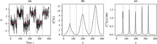
To infer how likely k is a potential change-point location, we consider all symmetric local windows that centered at k and define the score function according to (3.5) as (3.8) $${\text{T}}_n^{(\text{C})}(k)=\underset{\lfloor nϵ\rfloor \le d\le n}{\text{sup}}{\text{T}}_n^{(\text{C})}(k|k-d,k+1+d),$$(3.8) where $ϵ=0.1$. In Figure 1, the proposed score function (3.8) is compared with Shao and Zhang (2010) method. Clearly, ${\text{T}}_n^{(\text{C})}(·)$ achieves the local maxima near all true change-point locations, while ${\text{S}}_n^{(1)}(·)$ does not. Because the ${\text{S}}_n^{(1)}$ self-normalizers are not localized, they include data containing change points and are, therefore, inflated by other changes. Other possible reasons include reduced change-point detection capacity of the global CUSUM because of other changes and nonmonotonic change-point configuration. As a remark, the under-performance of ${\text{S}}_n^{(1)}$ comes with the benefit of smaller computational complexity; for more discussion; see Section 4.1. Finally, we obtain the proposed test statistic by aggregating the scores ${\text{T}}_n^{(\text{C})}(k)$ across k as follows: (3.9) $$\begin{array}{c}{\text{T}}_n^{(\text{C})}=\frac{1}{n-2\lfloor ϵn\rfloor -1}\sum _{k=\lfloor ϵn\rfloor +1}^{n-\lfloor ϵn\rfloor -1}{\text{T}}_n^{(\text{C})}(k),\hfill \end{array}$$(3.9) which captures the effects of all potential change points. For $j=1,\dots ,M$, define ${\pi }_j=k_j/n$ and ${\Delta }_j={\mu }_{k_j+1}-{\mu }_{k_j}$ be the jth relative change-point time and the corresponding change, respectively. Theorem 3.1 states the limiting distribution and the consistency of ${\text{T}}_n^{(\text{C})}$.

Fig. 1 (a) A realization of data (black solid line) with 5 change-points (blue dashed lines) and its mean function (red solid line). (b) Shao and Zhang’s (2010) score function ${\text{S}}_n^{(1)}(k)$. (c) The proposed score function ${\text{T}}_n^{(\text{C})}(k)$.

Theorem 3.1

(Limiting distribution and consistency). Suppose Assumption 2.1 is satisfied. (i) Under H₀, ${\text{T}}_n^{(\text{C})}\stackrel{\text{d}}{\to }\mathbb{T}$ for any $0<ϵ<1/2$, where (3.10) $$\mathbb{T}={(1-2ϵ)}^{-1}{\int }_{ϵ}^{1-ϵ}\underset{\delta >ϵ}{\text{sup}}\frac{\mathbb{L}{(t|t-\delta ,t+\delta )}^2}{\mathbb{V}(t|t-\delta ,t+\delta )} \text{d}t,$$(3.10) (3.11) $$\begin{array}{c}\mathbb{L}(t|{\tau }_1,{\tau }_2)=\frac{1}{{({\tau }_2-{\tau }_1)}^{1/2}}[\mathbb{B}(t)-\mathbb{B}({\tau }_1)\\ -\frac{t-{\tau }_1}{{\tau }_2-{\tau }_1}\left\{\mathbb{B}({\tau }_2)-\mathbb{B}({\tau }_1)\right\}],\end{array}$$(3.11) (3.12) $$\begin{array}{c}\mathbb{V}(t|t-\delta ,t+\delta )=\frac{1}{4\delta }\{{\int }_{t-\delta }^t\mathbb{L}{(\tau |t-\delta ,t)}^2 \text{d}\tau \\ +{\int }_t^{t+\delta }\mathbb{L}{(\tau |t,t+\delta )}^2 \text{d}\tau \}.\end{array}$$(3.12)

(ii) Under $H_{\ge 1}$, if there exist $j\in \{1,\dots ,M\}$ and C > 0 such that the jth change-point time satisfies $ϵ<\text{min}({\pi }_j-{\pi }_{j-1},{\pi }_{j+1}-{\pi }_j)$ and the corresponding jth change magnitude satisfies $\left|{\Delta }_j\right|=|{\mu }_{k_j+1}-{\mu }_{k_j}|>C$ as $n\to \infty$, then $\underset{n\to \infty }{\text{lim}}{\text{T}}_n^{(\text{C})}=\infty$ in probability.

The test statistic ${\text{T}}_n^{(\text{C})}$ has a pivotal limiting distribution under H₀, the quantiles of which can be found by simulation; see Table 1. See also Section 4 for more discussion on the critical value adjustment procedure for handling strong serial correlation when the sample size is small. Under $H_{\ge 1}$, the test is of power 1 asymptotically if the change magnitude is at least a nonzero constant. Theorem 3.2 concerns a local alternative hypothesis that contains change points with diminishing change magnitudes.

Table 1. Simulated quantiles of $\mathbb{T}$, that is, the limiting distribution of ${\text{T}}_n^{(\text{C})}$.

$\mathsf{P}(\mathbb{T}\le t)$	90%	95%	99%
t	17.6	19.6	23.7

Theorem 3.2

(Local limiting power). Under $H_{\ge 1}$, parameterize the jth change magnitude $|{\Delta }_j(n)|=|{\mu }_{k_j+1}-{\mu }_{k_j}|$ as a function of n. If there exist $j\in \{1,\dots ,M\}$ and $0.5<\kappa \le 1$ such that the jth change point satisfies $ϵ<\text{min}({\pi }_j-{\pi }_{j-1},{\pi }_{j+1}-{\pi }_j)$ and $|{\Delta }_j(n)|\asymp n^{\kappa -1}$ as $n\to \infty$, then $\underset{n\to \infty }{\text{lim}}{\text{T}}_n^{(\text{C})}=\infty$ in probability.

Motivated by Figure 1(c), a natural change-point set estimator $\widehat{\Pi }$ can be intuitively obtained from the points corresponding to the local maxima of the general score functions ${\text{T}}_n^{(\text{D})}(·)$ in (3.5). Specifically, the estimator is defined as (3.13) $$\begin{array}{c}{\widehat{\Pi }}^{(\text{D})}=\{\frac{k}{n}\in \left\{\frac{\lfloor nϵ\rfloor }{n},\dots ,\frac{n-\lfloor nϵ\rfloor }{n}\right\}:{\text{T}}_n^{(\text{D})}(k)\\ =\underset{{}_{k-\lfloor nϵ\rfloor <j\le k+\lfloor nϵ\rfloor }}{\text{max}}{\text{T}}_n^{(\text{D})}(j),\hspace{1em}{\text{T}}_n^{(\text{D})}(k)>\varrho \},\end{array}$$(3.13) where ϱ is a decision threshold and D is the global change-detecting process. In particular, if the CUSUM process is used, that is, $\text{D}=\text{C}$, Lemma 3.3 and Theorem 3.4 show the consistency of the proposed point estimator, ${\widehat{\Pi }}^{(\text{C})}$.

Lemma 3.3.

Let π_j be the jth relative change point, k_j be the jth change-point time such that $k_j/n\to {\pi }_j$ as $n\to \infty$ for $j=1,\dots ,M$, $k_0=0$, and $k_{M+1}=n$. Let h be any non-change-point time such that $|h/n-{\pi }_j|\to c>0$ as $n\to \infty$ for all j. Define $\mathsf{E}(X_i)=\mu +{\sum }_{j=1}^M{\Delta }_j\mathbb{1}(i/n>{\pi }_j)$. If ${\pi }_j-{\pi }_{j-1}>ϵ$ and ${\Delta }_j\asymp n^{{\kappa }_j-1}$ as $n\to \infty$, where $0.5<{\kappa }_j\le 1$ for all j, then for ${\zeta }_{n,j}=o(n^{2{\kappa }_j-1})$, $$\mathsf{P}\left\{{\text{T}}_n^{(\text{C})}(k_j)>{\zeta }_{n,j}\right\}\to 1\hspace{1em}\text{and}\hspace{1em}\mathsf{P}\left\{{\text{T}}_n^{(\text{C})}(h)>{\zeta }_{n,j}\right\}\to 0.$$

Theorem 3.4.

Assume that for all $j=1,\dots ,M$ where M is a finite constant, ${\pi }_j-{\pi }_{j-1}>ϵ$ and ${\Delta }_j\asymp n^{{\kappa }_j-1}$ as $n\to \infty$ where $0.5<{\kappa }_j\le 1$. Let ${\widehat{\pi }}_1^{(\text{C})}<{\widehat{\pi }}_2^{(\text{C})}<\cdots <{\widehat{\pi }}_{\widehat{M}}^{(\text{C})}$ be the elements of ${\widehat{\Pi }}^{(\text{C})}$. If $\varrho =o(n^{2\overline{\kappa }-1})$ where $\overline{\kappa }={\text{min}}_{j=1,\dots ,M}{\kappa }_j$, then for any small enough $\eta >0$ such that $\eta <ϵ$, $$\mathsf{P}\left\{\underset{{}_{j\prime =1,\dots ,M}}{\text{max}}\underset{{}_{j=1,\dots ,\widehat{M}}}{\text{min}}|{\pi }_{j\prime }-{\widehat{\pi }}_j^{(\text{C})}|>\eta \right\}\to 0.$$

By Lemma 3.3, the optimal threshold, ϱ, depends on the unknown change magnitudes. If the sizes of the changes are further assumed to be O(1), then we can set $\varrho =c{n}^{\upsilon }$ with $0<\upsilon <1$. Theoretically, it is challenging to derive an optimal choice of c and $\upsilon$ without a specific cost function that trades off the accuracy and size of ${\widehat{\Pi }}^{(\text{C})}$. It is possible to select $(c,\upsilon )$ across a class of change-point models through a large-scale simulation. As point estimation is beyond the scope of this article, we leave it as an open question for further study. From our experience, choosing $\varrho =\sqrt{n}$ yields a reasonable result. Because the score functions are computed during the computation of the proposed test statistics ${\text{T}}_n^{(\text{C})}$, the point estimator can be directly computed.

Remark 3.2

(Improving point estimation). The change-point estimation may be improved by further integrating other screening algorithms, for example, the screening and ranking algorithm (Niu and Zhang 2012) and the scanning procedure proposed by Yau and Zhao (2016), to perform model selection in order to avoid overestimating the number of change points. Alternatively, our proposed test can be applied to stepwise estimation, for example, binary segmentation (Vostrikova 1981), wild binary segmentation (Fryzlewicz 2014), and SNCP (Zhao, Jiang, and Shao 2021); see Section G of the supplement for information on how to integrate our method with existing screening methods.

3.3 Outlier-Robust Statistics

An outlier-robust nonparametric change-point test can be constructed using the Wilcoxon two-sample statistic. The corresponding ${\text{D}}_n(·)$ is (3.14) $$\begin{array}{c}{\text{W}}_n(\lfloor nt\rfloor )=\frac{1}{n^{3/2}}\sum _{i=1}^{\lfloor nt\rfloor }\sum _{j=\lfloor nt\rfloor +1}^n\left({\mathbb{1}}_{\{X_i\le X_j\}}-\frac{1}{2}\right)\\ =n^{-3/2}\left(\sum _{i=1}^{\lfloor nt\rfloor }{R}_i-\frac{\lfloor nt\rfloor }{n}\sum _{i\prime =1}^n{R}_{i\prime }\right),\end{array}$$(3.14) for $t\in [0,1]$, where $R_i={\sum }_{j=1}^n{\mathbb{1}}_{\{X_j\le X_i\}}$ is the rank of X_i when there is no tie in $X_1,\dots ,X_n$. It is assumed that the data are weakly dependent and can be represented as a functional of an absolutely regular process. Under some mixing conditions, we have $\{{\text{W}}_n(\lfloor nt\rfloor )\}\Rightarrow {\sigma }_{\text{W}}\left\{\mathbb{B}(t)-t\mathbb{B}(1)\right\}$, where ${\sigma }_{\text{W}}^2=\sum _{k\in \mathbb{Z}}\text{cov}\left\{F(X_0),F(X_k)\right\}$ and $F(·)$ is the distribution function of X₁ with a bounded density; see Theorem 3.1 in Dehling et al. (2015). From the principles in Section 3.1, we may use (3.14) to construct a self-normalized multiple-change-point Wilcoxon test and eliminate the nuisance parameter ${\sigma }_{\text{W}}$ by using the test statistic ${\text{T}}_n^{(\text{W})}={\text{T}}_n^{(\text{W})}[\text{max},\text{mean}]$; see the corollary below.

Corollary 3.5

(Limiting distribution of ${\text{T}}_n^{(\text{W})}$). Under the regularity conditions in Theorem 3.1 of Dehling et al. (2015) and H₀, we have ${\text{T}}_n^{(\text{W})}\stackrel{\text{d}}{\to }\mathbb{T}$.

The Hodges–Lehmann statistic is another popular alternative to the CUSUM statistic in (2.3). Its global change-detecting process is (3.15) $$\begin{array}{c}{\text{H}}_n(\lfloor nt\rfloor )=n^{-3/2}\lfloor nt\rfloor (n-\lfloor nt\rfloor )\\ \text{median}\left\{(X_i-X_j):1\le i\le \lfloor nt\rfloor <j\le n\right\},\end{array}$$(3.15) for $t\in [0,1]$, where $\text{median}(\mathcal{S})$ denotes the sample median of a set $\mathcal{S}$. It outperforms the CUSUM test under skewed and heavy-tailed distributions. Under the regularity conditions in Dehling, Fried, and Wendler (2020), we have $\{H_n(\lfloor nt\rfloor )\}\Rightarrow {\sigma }_{\text{H}}u{(0)}^{-1}\{\mathbb{B}(t)-t\mathbb{B}(1)\}$, where $u(x)={\int }_{\mathbb{R}}f(y)f(x+y) \text{d}y,{\sigma }_{\text{H}}^2=\sum _{k\in \mathbb{Z}}\text{cov}\{F(X_0),F(X_k)\}$, f is the density of X₁, and F is the distribution function of X₁. Similarly, we can apply the Hodges–Lehmann statistic to test for the existence of multiple change points. The corresponding test statistic is ${\text{T}}_n^{(\text{H})}={\text{T}}_n^{(\text{H})}[\text{max},\text{mean}]$. Its limiting distribution is presented in Corollary 3.6. To our knowledge, there is no existing self-normalized tests use the Hodges–Lehmann statistic. It is included to demonstrate the generality of the proposed self-normalization framework and to detect change points in heavy-tailed data.

Corollary 3.6

(Limiting distribution of ${\text{T}}_n^{(\text{H})}$). Under the regularity conditions in Theorem 1 of Dehling, Fried, and Wendler (2020) and H₀, we have ${\text{T}}_n^{(\text{H})}\stackrel{\text{d}}{\to }\mathbb{T}$.

3.4 Extension for Testing Change in General Parameters

Instead of testing changes in mean, one may be interested in other quantities, for example, variances, quantiles and model parameters. Let ${\theta }_i=P(F_i^{(h)})\in {\mathbb{R}}^q$, where $h\in \mathbb{N},P(·)$ is a functional, $F_i^{(h)}$ is the joint distribution function of $Y_i={(X_i,\dots ,X_{i+h-1})}^{⊺}$ for $i=1,\dots ,n-h+1$ and $q\in \mathbb{N}$. For example, for h = 1, ${\mu }_i={\int }_{-\infty }^{\infty }x \text{d}{F}_i^{(1)}(x)$ and ${\sigma }_i^2={\int }_{\mathbb{R}}{x}^2 \text{d}{F}_i^{(1)}(x)-{\{{\int }_{\mathbb{R}}x \text{d}{F}_i^{(1)}(x)\}}^2$ are the marginal mean and variance at time i, respectively. For h = 2, the lag-1 autocovariance at time i is ${\gamma }_i(1)={\int }_{{\mathbb{R}}^2}(x_i-{\mu }_i)(x_{i-1}-{\mu }_{i-1}) \text{d}{F}_i^{(2)}(x_{i-1},x_i)$. The hypotheses in (2.1) and (3.1) are redefined by replacing μ_i’s by θ_i’s. A possible global change-detecting process is (3.16) $${\text{G}}_n(\lfloor nt\rfloor )=\frac{\lfloor nt\rfloor (n-\lfloor nt\rfloor )}{n^{3/2}}\left({\widehat{\theta }}_{1,\lfloor nt\rfloor }-{\widehat{\theta }}_{\lfloor nt\rfloor +1,n}\right),$$(3.16) for $t\in [0,1]$; see, for example, Shao (2010), Shao and Zhang (2010), and Shao (2015). If ${\widehat{\theta }}_{i,j}={(j-i+1)}^{-1}{\sum }_{t=i}^j{X}_t$, then ${\text{G}}_n(·)={\text{C}}_n(·)$. Therefore, (3.16) generalizes (2.3) from testing changes in μ_i’s to testing changes in θ_i’s. The final test statistic is ${\text{T}}_n^{(\text{G})}={\text{T}}_n^{(\text{G})}[\text{max},\text{mean}]$.

The limiting distribution of (3.16) requires standard regularity conditions in handling statistical functionals. Based on the sample $Y_s,\dots ,Y_e$, define the empirical distribution of Y_i’s by ${\widehat{F}}_{s,e}^{(h)}={(e-s+1)}^{-1}{\sum }_{i=s}^e{\delta }_{Y_i}$, where δ_y is a point mass at $y\in {\mathbb{R}}^h$. Assume that ${\widehat{\theta }}_{s,e}=P({\widehat{F}}_{s,e}^{(h)})$ is asymptotically linear in the following sense, as $e-s\to \infty$: (3.17) $$P({\widehat{F}}_{s,e}^{(h)})=P(F^{(h)})+{(e-s+1)}^{-1}\sum _{i=s}^e\text{IF}(Y_i|P,F^{(h)})+R_{s,e},$$(3.17) where $R_{s,e}$ is a remainder term, $F^{(h)}=F_s^{(h)}=\cdots =F_e^{(h)}$, and $\text{IF}(y|P,F^h)=\underset{ϵ\to 0}{\text{lim}}\{P((1-ϵ)F^h+ϵ {\delta }_y)-P(F^h)\}/ϵ$ is the influence function; see Wasserman (2006).

Corollary 3.7

(Limiting distribution of ${\text{T}}_n^{(\text{G})}$). For $t\in [0,1]$ and $h\in \mathbb{N}$, define $I_n(\lfloor nt\rfloor )=n^{-1/2}{\sum }_{i=1}^{\lfloor nt\rfloor }\text{IF}(Y_i|P,F^{(h)})$, where $F^{(h)}=F_1^{(h)}=\cdots =F_{n-h+1}^{(h)}$ under H₀. Suppose that (i) $\mathsf{E}\{\text{IF}(Y_i|P,F^h)\}=0$ for all i, (ii) $\{I_n(t):t\in [0,1]\}\Rightarrow \{{\sigma }_{\text{G}}{\mathbb{B}}^{(q)}(t):t\in [0,1]\}$ for some positive definite matrix σ_G and ${\mathbb{B}}^{(q)}(·)$ is q-dimensional standard Brownian motion, where $q\in \mathbb{N}$, and (iii) $\underset{k=1,\dots ,n-1}{\text{sup}}\left|R_{1:k}\right|+\left|R_{(k+1):n}\right|=o_p(n^{-1/2})$. Then ${\text{T}}_n^{(\text{G})}\stackrel{\text{d}}{\to }{\mathbb{T}}^{(q)}$, where $$\begin{array}{c}{\mathbb{T}}^{(q)}={(1-2ϵ)}^{-1}{\int }_{ϵ}^{1-ϵ}\underset{\delta >ϵ}{\text{sup}}{\mathbb{L}}^{(q)}{(t|t-\delta ,t+\delta )}^{\text{T}}{\mathbb{V}}^{(q)}{(t|t-\delta ,t+\delta )}^{-1}\\ \mathrm{\hspace{1em}}\mathrm{\hspace{1em}}{\mathbb{L}}^{(q)}(t|t-\delta ,t+\delta ) \text{d}t,\end{array}$$where ${\mathbb{L}}^{(q)}$ is defined as $\mathbb{L}$ in (3.11) but with $\mathbb{B}(·)$ being replaced by ${\mathbb{B}}^{(q)}(·)$; and ${\mathbb{V}}^{(q)}$ is defined as $\mathbb{V}$ in (3.11) but with $\mathbb{L}{(·|·,·)}^2$ being replaced by ${\mathbb{L}}^{(q)}{(·|·,·)}^{\otimes 2}$. In particular, ${\mathbb{T}}^{(1)}=\mathbb{T}$.

4 Discussion and Implementation

4.1 Comparison with Existing Methods

Shao and Zhang (2010) extended the self-normalized one-change-point test (2.4) to a supervised multiple-change-point test tailored for testing m change-points, where m is pre-specified. The test statistic is (4.1) $${\text{S}}_n^{(m)}=\underset{(k_1,\dots ,k_m)\in {\Omega }_n^{(m)}(ϵ)}{\text{sup}}\sum _{j=1}^m{\text{T}}_n^{(\text{C})}(k_1|k_{j-1},k_{j+1}),$$(4.1) where ${\Omega }_n^{(m)}(ϵ)=\{k_1,\dots ,k_m:j\in \{1,\dots ,m\},\lfloor ϵn\rfloor \le$ $\text{min}(k_j-k_{j-1},k_{j+1}-k_j)\},k_0=1$, and $k_{m+1}=n$. The trimmed region ${\Omega }_n^{(m)}(ϵ)$ prevents estimates from being computed with too few observations. Later, Zhang and Lavitas (2018) proposed an unsupervised self-normalized multiple-change-point test that bypasses specifying m and is defined as, (4.2) $$\begin{array}{c}{\text{Z}}_n=\underset{(k_1,k_2)\in {\Omega }_n^{(2)}(ϵ)}{\text{sup}}{\text{T}}_n^{(\text{C})}(k_1|1,k_2)\\ \hspace{1em}+\underset{(k_1,k_2)\in {\Omega }_n^{(2)}(ϵ)}{\text{sup}}{\text{T}}_n^{(\text{C})}(k_2|k_1,n).\end{array}$$(4.2)

Although ${\text{S}}_n^{(m)},{\text{Z}}_n$ and ${\text{T}}_n^{(\text{C})}$ use LSN CUSUM statistics, that is, ${\text{T}}_n^{(\text{C})}(k|s,e)$, as building blocks, they have different restrictions on the local windows and aggregate the LSN statistics in different ways. The Shao and Zhang (2010) multiple-change-point test has strict control over the m local windows because the boundaries of a window relate to preceding and subsequent windows. If the number of change points is misspecified, some windows may not contain only one change point. If m < M, the self-normalizers are not robust to changes. If m > M, some degrees of freedom are lost trying to detect change points that do not exist. Both cases may lead to a significant loss of power. Moreover, their computational cost increases exponentially with m. The Zhang and Lavitas’s (2018) approach sets the left end of the window to 1 in the forward scan, and the right end to n in the backward scan. Therefore, their approach tends to scan for the first change point $k_1\in [1,e]$ and the last change point $k_M\in [s,n]$ for some e and s, which may lead to a loss of power; see Section 5.2. In contrast, our approach scans for all possible change points because windows can start and end at any time with the same computation complexity; see Section C.9 of the supplement. The score function at each time takes O(n) steps to compute and O(1) spaces to store using recursive computation. Because the test statistic is computed as a function of O(n) scores, it has a computational cost of $O(n^2)$ and a memory requirement of O(n). Table 2 summarizes the comparison. As a remark, the self-normalized segmentation algorithms proposed by Jiang, Zhao, and Shao (2021) and Zhao, Jiang, and Shao (2021) are also based on localized CUSUM contrast-type change-detecting statistics. In the testing stage, a nested window set is introduced to control the computational cost by considering a finite set of windows. In contrast, we develop recursive LSN statistics that consider all symmetric windows with sizes greater than ϵ. Therefore, our method considers all possible windows with size greater than $\lfloor ϵn\rfloor$ and possibly increases power.

Table 2. Comparisons between various different change-point tests in terms of (a) finite-sample size accuracy with respect to the nominal Type-I error rate; (b) power under several change-point numbers M; (c) time complexity of computing the test statistics based on a sample of size n; (d) robustness against outliers; and (e) requirements of computing a long-run variance estimate ${\widehat{\sigma }}_n^2$ and specifying a target number of change points m, where ${\widehat{\sigma }}_n^2$ is assumed to be computed in O(n) steps.

	(a) Size accuracy	(b) Powerfulness		(c) Time complexity	(d) Robustness	(e) Requirement
		M = 1	M > 1			${\widehat{\sigma }}_n^2$	m
${\text{KS}}_n$	Low	High	Low	O(n)	Low	Yes	No
${\text{S}}_n^{(1)}$	High	High	Low	O(n)	Low	No	Yes
${\text{S}}_n^{(m)}$	Medium	Medium	Depends on m	$O(n^m)$	Low	No	Yes
${\text{Z}}_n$	Medium	Medium	Medium	$O(n^2)$	Low	No	No
${\text{T}}_n^{(\text{C})}$	High	High	High	$O(n^2)$	Low	No	No
${\text{T}}_n^{(\text{W})}$	High	High	High	$O(n^2)$	High	No	No
${\text{T}}_n^{(\text{H})}$	High	High	High	$O(n^3\hspace{0.17em}\text{log}\hspace{0.17em}n)$	High	No	No

NOTE: The comparisons in (a) and (b) are based on our simulation results in Section 5 and the supplement.

4.2 Finite-n Adjusted Critical Values

In the time series context, the accuracy of the invariance principle, that is, Assumption 2.1, may deteriorate when the sample size is small (Kiefer and Vogelsang 2005). Therefore, the asymptotic theory in, for example, Theorem 3.1, may not apply when serial dependency is strong and the sample size is small. It may lead to severe size distortion, observed in both existing self-normalized and non-self-normalized methods, including the proposed tests; see Section 5 and Section C.13 of the supplement for simulation evidences. For the multiple-change-point problem (3.1) in mean, a finite-sample adjusted critical value procedure based on the strength of serial dependency is proposed to mitigate this problem.

We propose to compute a critical value $c_{\alpha }(n,\rho )$ by matching the autocorrelation function (ACF) at lag one ρ and n for various specified levels of significance $\alpha \in (0,1)$. The values of $c_{\alpha }(n,\rho )$ are tabulated in Section D of the supplement for $\alpha \in \{0.01,0.05,0.1\},n\in \{100,200,\dots ,1000,2000,\dots ,10000\}$, and $\rho \in \{0,\pm 0.1,\dots ,\pm ,0.9\}$. The testing procedure is outlined as follows.

1. Compute the sample lag-1 ACF $\widehat{\rho }$ of ${\{X_{i+b_n}-X_i\}}_{i=1}^{n-b_n}$, where $b_n=\lfloor n^{1/3}\rfloor$ is the differencing parameter.

2. Obtain the critical value $c_{\alpha }(n,\widehat{\rho })$ by matching n and ρ. Use linear interpolation if n and/or $\widehat{\rho }$ do not lie in the grids.

3. Reject the null if ${\text{T}}_n^{(\aleph )}>c_{\alpha }(n,\widehat{\rho })$, where $\aleph \in \{\text{C},\text{W},\text{H},\text{G}\}$.

The adjustment procedure borrows from the idea of bootstrap-based critical value simulation procedures; see for example, Zhou (2013) and Pešta and Wendler (2020). The limiting distribution is pivotal by Theorem 3.1 and Corollaries 3.5–3.7. Therefore, the critical value simulation procedure can be performed prior to the computation of the test statistic. Because $\widehat{\rho }$ depends on the differenced data with a suitable lag, the change points (if any) have negligible effect on $\widehat{\rho }$.

The consistency of $\widehat{\rho }$ is developed on the following framework: Let $X_i={\mu }_i+Z_i$, where μ_i’s are deterministic and Z_i’s are zero-mean stationary noises. Define $Z_i=g(\dots ,{\epsilon }_{i-1},{\epsilon }_i)$, where ${\epsilon }_i$‘s are independent and identically distributed ($\text{iid}$) random variables and g is some measurable function. Let ${\epsilon }_i^{\prime }$ be an $\text{iid}$ copy of ${\epsilon }_i$ and $Z_i^{\prime }=g(\dots ,{\epsilon }_{-1},{\epsilon }_0^{\prime },{\epsilon }_1,\dots ,{\epsilon }_i)$. For p > 1 and ${\Vert Z_i\Vert }_p<\infty$, the physical dependence measure (Wu 2011) is defined as ${\lambda }_p(i)={\Vert Z_i-Z_i^{\prime }\Vert }_p$, where ${\Vert ·\Vert }_p={(\mathsf{E}|·{|}^p)}^{1/p}$. Theorem 4.1 states that $\widehat{\rho }$ is a consistent estimator even under a large number of change points M. In particular, if $b_n=\lfloor n^{1/3}\rfloor$ and $\left|{\Delta }_{*}\right|<\infty$, then Theorem 4.1 guarantees that $\widehat{\rho }$ is consistent for ρ if $M=o(n^{2/3})$. The proposed adjustment only affects the finite-sample performance because the critical value $c_{\alpha }(n,\rho )$ is a constant as a function of ρ when $n\to \infty$.

Theorem 4.1.

Assume that $\mathsf{E}(Z_1^4)<\infty$ and ${\sum }_{i=1}^{\infty }{\lambda }_4(i)<\infty$. Define $\left|{\Delta }_{*}\right|=\underset{1\le j\le M}{\text{sup}}\left|{\Delta }_j\right|$. Let b_n be an $\mathbb{N}$-valued sequence. If $b_n/n+1/b_n+(b_{n}M/n){\Delta }_{*}^2\to 0$ as $n\to \infty$, then $\widehat{\rho }\stackrel{\text{pr}}{\to }\rho$.

Although it is possible to match the ACF at a higher lag, the AR(1) model is considered to balance the accuracy and the computational cost; see Section C.13 of the supplement. The sensitivity analysis of the differencing parameter b_n in Section C.14 of the supplement also verifies that the choice has a minimal effect on the performance of the tests. The simulation result shows that the tests have a remarkably accurate size even when the true model is not the AR(1) model; see Section 5 and Section C of the supplement. It indicates that the selected AR(1) model has certain explanatory power. If another approximation model is more appropriate for a specific application, then the AR(1) model should be replaced. Users may choose between the standard testing procedure using Table 1 or the proposed adjustment, if it is appropriate.

5 Simulation Experiments

5.1 Setting and Overview

Throughout Section 5, the experiments are designed as follows. The time series is generated from a signal-plus-noise model: $X_i={\mu }_i+Z_i$. The values of μ_i’s will be specified in Sections 5.2 and 5.3. The zero-mean noises Z_i’s are simulated from a stationary bilinear autoregressive (BAR) model: (5.1) $$Z_i=(\varpi +\vartheta {\epsilon }_i)Z_{i-1}+{\epsilon }_i,\hspace{1em}i=1,\dots ,n,$$(5.1) where ${\epsilon }_i$‘s are independent standard normal random variables, and $\varpi ,\vartheta \in \mathbb{R}$ such that ${\varpi }^2+{\vartheta }^2<1$. The BAR model is a class of nonlinear time series models that have been extensively studied in the literature; see, for example, Granger and Anderson (1978), Rao (1981), and Rao and Gabr (1984). The bilinear time series model is widely used in the fields of control theory (Bruni, DiPillo, and Koch 1974), econometrics (Weiss 1986), and seismology (Dargahi-Noubary, Laycock, and Rao 1978), which the phenomenon of occasional sharp spikes occurs in sample paths. Similar findings are obtained under other noise models, including the autoregressive-moving-average model, threshold AR model, and absolute value nonlinear AR model. Because of space constraints, these results are presented in to the supplement. The critical value is chosen according to the adjustment procedure described in Section 4.2.

5.2 Size and Power

In this section, we examine the size and power of different tests when there exist various numbers of change points. Following the suggestion of Huang, Volgushev, and Shao (2015) and Zhang and Lavitas (2018), we choose $ϵ=0.1$ in ${\text{S}}_n^{(2)},{\text{S}}_n^{(3)},{\text{Z}}_n$ and in our proposed tests for a fair comparison. Suppose that the change points are evenly spaced and the mean change directions are alternating (increasing or decreasing): (5.2) $${\mu }_i=\Delta \sum _{j=1}^M{(-1)}^{j+1}{\mathbb{1}}_{\{i/n>j/(M+1)\}},$$(5.2) where $M\in \{1,\dots ,6\}$ denotes the number of change points, and $\Delta \in \mathbb{R}$ controls the magnitude of the mean changes. Then, ${\mu }_i\equiv 0$ under H₀.

All tests are computed at the nominal size $\alpha =5\%$. The null rejection rates $\widehat{\alpha }$, for sample sizes $n\in \{200,400\}$, are presented in Table 3. To summarize the result, we further report the sample root mean squared error (RMSE) of $\widehat{\alpha }$ over all cases of $\vartheta =0.8,-0.5,0.5,0.8$ and $\varpi =-0.8,-0.5,-0.3,0,0.3,0.5,0.8$ for each test and each n. Specifically, $${\text{RMSE}}_n={\left[|\mathcal{H}{|}^{-1}\sum _{(\vartheta ,\varpi )\in \mathcal{H}}\{{\widehat{\alpha }}_n(\vartheta ,\varpi )-\alpha {\}}^2\right]}^{1/2},$$where $\mathcal{H}$ is the set of $(\vartheta ,\varpi )$ used in the simulation, $\left|\mathcal{H}\right|$ is the cardinality of $\mathcal{H}$, and ${\widehat{\alpha }}_n(\vartheta ,\varpi )$ is the empirical size under the BAR model with parameter ϑ and ϖ with sample size n. The self-normalized tests generally have a more accurate size than the non-self-normalized test ${\text{KS}}_n$. This finding is consistent with that of Shao (2015). The self-normalized approach is a special case of the fixed bandwidth approach with the largest possible bandwidth and thus achieves the smallest size distortion, as observed by Kiefer and Vogelsang (2002). In comparison, ${\text{T}}_n^{(\text{W})}$ and ${\text{T}}_n^{(\text{H})}$ control the size most accurately among the self-normalized tests. In particular, our proposed tests have the least severe under-size problem, observed in existing self-normalized tests (i.e., ${\text{S}}_n^{(1)}$, ${\text{S}}_n^{(2)},{\text{S}}_n^{(3)}$, and ${\text{Z}}_n$) when $\varpi <0$. Moreover, the test proposed by Shao and Zhang (2010), ${\text{S}}_n^{(m)}$, suffers from an increasing size distortion as m increases. This finding is consistent with that of Zhang and Lavitas (2018). The fact that ${\text{T}}_n^{(\text{W})}$ and ${\text{T}}_n^{(\text{H})}$ outperform ${\text{T}}_n^{(\text{C})}$ can be attributed to the outlier robustness of rank and order statistics. This advantage is particularly noticeable in bilinear time series, as this model is well known for producing sudden high amplitude oscillations that mimic structures in, for example, explosion and earthquake data in seismology; see Section 5.2 of Rao and Gabr (1984). However, in the more standard ARMA models, ${\text{T}}_n^{(\text{C})}$ performs as well as ${\text{T}}_n^{(\text{W})}$ and ${\text{T}}_n^{(\text{H})}$; see the supplement for the detailed results.

Table 3. Null rejection rates $\widehat{\alpha }$ at nominal size $\alpha =5\%$ under BAR model and mean function (5.2).

		n = 200								n = 400
ϑ	ϖ	${\text{KS}}_n$	${\text{S}}_n^{(1)}$	${\text{S}}_n^{(2)}$	${\text{S}}_n^{(3)}$	${\text{Z}}_n$	${\text{T}}_n^{(\text{C})}$	${\text{T}}_n^{(\text{W})}$	${\text{T}}_n^{(\text{H})}$	${\text{KS}}_n$	${\text{S}}_n^{(1)}$	${\text{S}}_n^{(2)}$	${\text{S}}_n^{(3)}$	${\text{Z}}_n$	${\text{T}}_n^{(\text{C})}$	${\text{T}}_n^{(\text{W})}$	${\text{T}}_n^{(\text{H})}$
0.8	0.5	14.4	7.5	9.6	5.3	7.6	1.1	4.0	3.4	11.3	5.3	5.3	3.1	5.4	0.8	3.8	3.3
	0.3	13.5	5.6	5.8	3.1	5.1	1.2	4.5	3.4	10.7	4.9	4.5	2.7	4.5	1.3	4.0	3.4
	0	15.4	4.7	2.8	1.3	2.4	2.3	5.6	4.6	10.6	4.8	3.7	1.9	3.0	2.1	4.1	3.7
	–0.3	23.9	4.6	1.7	0.4	1.5	2.1	7.8	6.3	15.6	3.9	2.1	0.8	1.9	2.1	5.6	5.0
	–0.5	31.2	3.9	1.6	0.4	1.2	2.0	7.7	7.1	25.6	4.5	1.4	0.3	1.4	1.4	6.4	6.3
0.5	0.8	31.8	11.9	26.1	27.2	27.1	3.6	11.0	9.0	31.8	8.0	14.9	12.8	14.3	2.2	5.7	3.6
	0.5	13.7	6.5	9.5	8.8	8.1	2.1	4.5	3.9	10.0	6.0	6.6	6.1	6.4	2.1	3.9	3.5
	0.3	11.0	5.1	5.5	4.9	5.6	3.0	5.0	4.6	7.6	4.8	5.7	4.1	5.2	2.7	4.5	4.1
	0	9.4	3.9	3.8	2.0	2.7	3.8	6.5	6.1	6.6	4.8	4.1	3.1	3.8	3.2	4.3	4.4
	–0.3	17.9	3.5	1.7	0.4	1.5	4.3	6.3	5.9	10.0	4.2	3.2	1.8	2.5	3.1	5.3	4.8
	–0.5	29.8	3.1	1.0	0.0	0.8	4.1	7.2	6.0	19.8	3.9	2.7	1.5	2.0	3.3	6.0	6.0
	–0.8	44.1	2.6	0.2	0.0	0.1	4.3	8.7	7.3	37.3	2.9	0.9	0.1	0.4	3.2	6.9	6.5
–0.5	0.8	29.8	10.1	24.0	27.7	24.8	2.8	11.4	8.5	29.3	8.2	11.9	9.6	12.4	1.6	4.9	3.6
	0.5	12.2	5.6	8.6	7.1	9.0	1.7	3.4	2.6	10.0	5.1	5.4	4.4	5.9	2.3	4.0	3.4
	0.3	9.3	4.9	6.3	3.6	5.8	2.4	3.7	3.4	7.4	4.3	5.3	3.7	4.6	3.2	4.1	3.6
	0	9.1	5.1	3.4	2.1	3.0	3.6	4.7	4.3	6.4	4.8	4.4	3.2	4.0	3.3	5.8	5.3
	–0.3	15.8	3.9	1.6	1.0	1.8	3.1	6.1	5.2	10.1	4.6	3.7	2.0	3.0	3.8	5.3	5.0
	–0.5	27.9	3.6	1.0	0.6	1.1	4.3	6.2	6.0	19.5	4.4	3.1	1.6	3.0	4.3	5.4	5.1
	–0.8	44.0	1.8	0.7	0.0	0.3	4.7	6.3	6.3	38.7	3.5	1.0	0.2	0.9	3.1	6.1	5.6
–0.8	0.5	13.6	7.4	7.4	4.5	6.3	0.8	3.1	2.5	11.0	6.2	4.5	2.8	3.9	1.1	3.2	2.5
	0.3	13.2	5.9	4.6	2.3	3.6	1.0	3.2	2.7	9.1	5.7	3.3	2.1	2.7	1.9	4.2	3.4
	0	14.4	5.1	2.6	1.1	2.4	1.3	4.1	3.2	11.2	4.5	3.6	1.6	3.1	2.4	5.8	5.1
	–0.3	21.1	5.4	1.9	0.5	1.3	1.6	6.3	4.7	17.9	4.9	2.4	1.0	1.8	2.7	6.8	5.5
	–0.5	31.4	5.2	1.3	0.2	1.3	1.9	8.3	7.0	28.2	5.6	1.9	0.5	1.4	2.1	6.0	5.2
${\text{RMSE}}_n$		18.9	2.2	6.5	7.4	6.8	2.7	2.5	1.8	15.1	1.2	3.2	3.6	3.3	2.7	1.0	1.2

NOTE: The sample ${\text{RMSE}}_n$ of $\widehat{\alpha }$ over all cases of ϑ and ϖ is computed for each test and each n. The values of $\widehat{\alpha }$ and RMSE are expressed in percentage. The effectiveness of the test in controlling the Type-I error increases with a decreasing ${\text{RMSE}}_n$.

The power curve against Δ is computed at 5% nominal size using 2¹⁰ replications with n = 200. Figure 2 displays the size-adjusted power when $\varpi =\vartheta =0.5$. The (unadjusted) power is presented in the supplement. The results with various values of ϖ and ϑ are similar, thus, they are presented in the supplement. Generally, ${\text{T}}_n^{(\text{W})}$ and ${\text{T}}_n^{(\text{H})}$ have the highest power. They outperform ${\text{T}}_n^{(\text{C})}$ because of their robustness against outliers. When only the CUSUM-type tests are considered, the non-self-normalized test ${\text{KS}}_n$ performs better than self-normalized tests when M = 1. However, when M > 1, ${\text{KS}}_n$ significantly under-performs because it is tailor-made for the AMOC alternative (2.2). Although ${\text{S}}_n^{(1)}$ has the highest power among the self-normalized CUSUM tests when M = 1, it suffers from the notorious non-monotonic power problem when M > 1 because its self-normalizer is not robust to multiple change points. Thus, ${\text{S}}_n^{(1)}$ is not a consistent test when M > 1.

Fig. 2 Size-adjusted power under BAR model with $\varpi =\vartheta =0.5$, n = 200 and mean function (5.2).

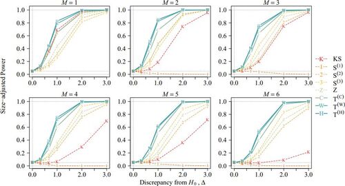
Surprisingly, our proposed test ${\text{T}}_n^{(\text{C})}$ outperforms the tests of Shao and Zhang (2010), ${\text{S}}_n^{(m)}$, even when M is well-specified. This finding demonstrates that it is not advantageous to know M because structural change can be identified by observing the data around it without looking at the entire segmented series. Moreover, as discussed in Section 4.1, ${\text{S}}_n^{(m)}$ defines the local windows restrictively. It accumulates errors if the boundaries of the local windows differ from the actual change points. It is also interesting to see that, compared with ${\text{S}}_n^{(1)}$, ${\text{S}}_n^{(2)}$, and ${\text{S}}_n^{(3)}$ are less sensitive to misspecification of M; however, they are still less powerful than our proposed tests.

5.3 Ability to Capture Effects of All Changes

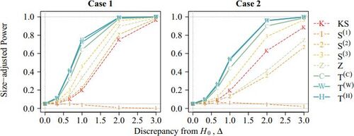
The proposed tests are robust against multiple change points compared with existing methods. Consider the three-change-point setting in which the magnitude of changes at the first and the last change points is only half that of the second change point. Specifically, define the mean function for case 1 as (5.2) with M = 3 and for case 2 as $${\mu }_i=\Delta \left\{\frac{1}{2}·{\mathbb{1}}_{\{i>\lfloor n/4\rfloor \}}-{\mathbb{1}}_{\{i>\lfloor 2n/4\rfloor \}}+\frac{1}{2}·{\mathbb{1}}_{\{i>\lfloor 3n/4\rfloor \}}\right\}.$$

From Figure 3, ${\text{Z}}_n$ and ${\text{S}}_n^{(2)}$ lose approximately half of their power in Case 2 compared with that in Case 1. In contrast, the power of our tests only decreases by 1/3 when $\Delta \le 1$, while it remains roughly the same when $\Delta \ge 2$. Therefore, our tests are more powerful and can capture a larger class of structural changes than existing methods. In contrast, ${\text{S}}_n^{(2)}$ and ${\text{Z}}_n$ tend to consider the first and/or the last change points.

Fig. 3 Size-adjusted power under the BAR model with $\varpi =\vartheta =0.5$, n = 200 and mean functions as in cases 1 and 2.

5.4 Change in General Parameters

In many applications, trends may exist in the data. Therefore, we consider the multiple-change-point problem in the mean and median trend models. Specifically, we consider the regression model: $\Phi (X_i)={\alpha }_i+{\beta }_i(i/n)$ with $\Phi (·)=\mathsf{E}(·)$ and $\Phi (·)=\text{median}(·)$ under the following multiple-change-point model: $$\begin{array}{c}{\alpha }_i={\Delta }_{\alpha ,0}+\sum _{j=1}^M{\Delta }_{\alpha ,j}\mathbb{1}(i/n>{\pi }_j)\hspace{1em}\text{and}\\ {\beta }_i={\Delta }_{\beta ,0}+\sum _{j=1}^M{\Delta }_{\beta ,j}\mathbb{1}(i/n>{\pi }_j)\end{array}$$for $i=1,\dots ,n$, where $M\in \mathbb{N},0<{\pi }_1<\cdots <{\pi }_M<1$, and ${\Delta }_{\alpha ,0},\dots ,{\Delta }_{\alpha ,M},{\Delta }_{\beta ,0},\dots ,{\Delta }_{\beta ,M}\in \mathbb{R}$. Note that $\Phi (·)=\mathsf{E}(·)$ and $\Phi (·)=\text{median}(·)$ refer to the mean trend and median trend models, respectively. Our goal is to test H₀ against $H_{\ge 1}$ with μ_i’s replaced by β_i’s.

To handle changes in general parameters, the global change-detecting process ${\text{G}}_n(·)$ in (3.16) is used. Let ${\widehat{\theta }}_{s:e}$ be an estimator of the common value of ${\beta }_s,\dots ,{\beta }_e$ based on observations $X_s,\dots ,X_e$ under H₀. The estimators ${\widehat{\theta }}_{s:e}$ are obtained using ordinary least-squares regression under the mean trend model; while they are obtained using quantile regression under the median trend model and computed by the R package “quantreg”. Let ${\text{T}}_n^{(\text{G},\text{mean})}$ and ${\text{T}}_n^{(\text{G},\text{med})}$ be the mean trend version and median trend version of the test statistics ${\text{T}}_n^{(\text{G})}$ in Section 3.4, respectively. In our simulation, we generate the data as $$\begin{array}{c}{X}_i=\Delta \sum _{j=0}^M\left\{\frac{(i-\lfloor jn/(M+1)\rfloor }{\lfloor n/(M+1)\rfloor }\wedge 1\right\}{\mathbb{1}}_{\{i/n>j/(M+1)\}}+Z_i,\\ \mathrm{\hspace{1em}}\mathrm{\hspace{1em}}i=1,\dots ,n,\end{array}$$where Z_i’s are simulated from the BAR model (5.1), $M\in \{1,\dots ,6\}$ denotes the number of change points, and $\Delta \in \mathbb{R}$ controls the magnitude of the changes. Briefly, the model implies an uptrend in mean and median before every odd index of change points until level Δ. After reaching Δ at odd change points, the trend shifts downward and decreases to 0 at the next change point. The empirical rejection rates are reported in Table 4. From the results, ${\text{T}}_n^{(\text{G},\text{mean})}$ suffers less severe under-size distortion than ${\text{T}}_n^{(\text{G},\text{med})}$. Both tests have decent powers in the multiple-change-point setting and significantly improve from n = 200 to n = 400. For reference, the size-adjusted power is also reported in Section C.11 of the supplement.

Table 4. Empirical rejection rates (%) of the mean and median trend tests, ${\text{T}}_n^{(\text{G},\text{mean})}$ and ${\text{T}}_n^{(\text{G},\text{med})}$, respectively, at 5% nominal size under the BAR model.

	${\text{T}}_n^{(\text{G},\text{mean})}$						${\text{T}}_n^{(\text{G},\text{med})}$
n	200			400			200			400
$\Delta \mathrm{\backslash }M$	1	3	6	1	3	6	1	3	6	1	3	6
	$\vartheta =0.5$ and $\varpi =0.5$
0	3.0	3.0	3.0	4.1	4.1	4.1	0.0	0.0	0.0	0.4	0.4	0.4
0.33	6.7	5.5	5.1	5.4	4.7	4.1	0.4	0.3	0.2	0.3	0.1	0.1
0.67	7.1	7.5	5.9	9.4	13.2	10.0	0.4	0.2	0.3	1.7	1.4	0.5
1	10.6	12.3	11.1	14.4	32.6	21.1	0.4	1.3	0.1	4.0	9.3	2.0
2	28.3	51.9	41.4	45.6	84.5	76.0	5.4	15.4	1.9	23.7	64.6	33.7
3	51.8	82.1	74.9	77.8	97.6	94.4	16.2	47.6	11.1	59.1	93.7	77.8
	$\vartheta =-0.5$ and $\varpi =-0.5$
0	2.6	2.6	2.6	2.1	2.1	2.1	0.0	0.0	0.0	0.0	0.0	0.0
0.33	4.7	14.6	7.2	6.5	23.8	8.9	0.6	0.6	0.2	0.4	0.7	0.3
0.67	10.7	57.2	25.9	26.2	82.3	59.1	0.7	2.5	0.3	1.2	8.7	1.0
1	30.2	91.2	67.7	59.2	99.2	96.9	1.7	8.0	0.7	5.5	29.3	4.5
2	93.0	100.0	100.0	100.0	100.0	100.0	23.3	55.2	15.8	53.5	96.0	71.2
3	100.0	100.0	100.0	100.0	100.0	100.0	65.2	93.1	62.8	93.7	99.9	98.6

6 Shanghai-Hong Kong Stock Connect turnover

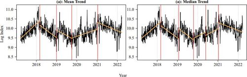
We use our proposed method to perform change-point analysis of the Shanghai-Hong Kong Stock Connect Southbound Turnover index (Bloomberg code: AHXHT index) from March 23, 2017 to March 22, 2022 (n = 1232). The data are retrieved from Bloomberg. The Stock Connect is a channel that allows mainland China and Hong Kong investors to access other stock markets jointly. The southbound line enables investors in mainland China to invest in the Hong Kong stock market. Studies have shown that the Stock Connect improves mutual market liquidity and capital market liberalization (Bai and Chow 2017; Huo and Ahmed 2017; Xu et al. 2020). Therefore, it is of practical interest, to determine whether change points exist in the Stock Connect Southbound daily turnover.

We investigate whether changes in trend exist in the log daily turnovers. Under the mean and median trend models, we consider the tests statistics ${\text{T}}_n^{(\text{G},\text{mean})}$ and ${\text{T}}_n^{(\text{G},\text{med})}$, specified in Section 5.4. The resulting test statistics are 47.46 and 40.64. Both p-values are less than 1%. The trend change-point location estimates are indicated by red vertical lines in Figure 4. The mean and median trend analyses agree on four estimated change points, estimated on March 7, 2018, January 24, 2019, October 2, 2019, and January 12, 2021. The median trend analysis detects an additional change point on May 25, 2020. The first change point is likely to be the China–United States trade war. After the trade war began in January 2018, the Stock Connect turnover displayed a downtrend. An uptrend is detected after 2019 until the COVID-19 events, while it stops after the beginning of 2021.

Fig. 4 Estimated (a) mean trend and (b) median trend change points are indicated by red vertical lines. The orange lines indicate the fitted regression lines within each region separated by the estimated change points. Data are retrieved from Bloomberg.

7 Conclusion

Our method improves existing change-point tests and has several advantages: (i) it has high power and size accuracy, (ii) it does not require specification of the number of change points nor consistent estimation of nuisance parameters, (iii) a consistent estimate of change points can be naturally produced, (iv) general change-detecting statistics, for example, rank and order statistics, can be used to enhance robustness, (v) it can test a change in general parameter of interest, and (vi) it applies to a wide range of time series models. Table 2 summarizes the properties of the proposed tests. Moreover, our proposed framework is driven by intuitive principles. If a single-change-detecting statistic is provided, our framework can generalize it to a multiple-change-detecting statistic. We anticipate that future works will apply our framework to non-time-series data, for example, spatial and spatial–temporal data.

8 Proofs of Theorems

Proof of Theorem

s 3.1 and 3.2. (i) Under H₀ and by the continuous mapping theorem, Assumption 2.1 implies that $\{{\text{C}}_n(\lfloor nt\rfloor ):t\in [0,1]\}\Rightarrow \{\sigma (\mathbb{B}(t)-t\mathbb{B}(1)):t\in [0,1]\}$. Note that ${\text{T}}_n^{(\text{C})}$ is a composite function of ${\text{C}}_n(·)$ through (3.2), (3.3), (3.4), (3.5), and (3.6), each of which is a continuous and measurable map. By the continuous mapping theorem, we obtain ${\text{T}}_n^{(\text{C})}\stackrel{\text{d}}{\to }\mathbb{T}$ in (3.10). The limiting distribution $\mathbb{T}$ is well-defined because ${\text{V}}_n^{(\text{C})}(k|k-d,k+1+d)$ converges to a nonnegative and nondegenerate distribution for any $\lfloor nϵ\rfloor \le d\le n$ and $\lfloor ϵn\rfloor +1\le k\le n-\lfloor ϵn\rfloor -1$, if $ϵ>0$.

(ii) For consistency, we consider the jth relative change-point time π_j such that the corresponding change magnitude satisfies $\left|{\Delta }_j\right|\asymp n^{\kappa -1}$, where $0.5<\kappa \le 1$. Let ${\Delta }_{*}={\Delta }_j$ and $k_{*}=\lfloor n{\pi }_j\rfloor$. Under this assumption, there exist $c\in {\mathbb{R}}^{+}$ and $3/2-\kappa \le {\rm Y}<1$ such that $ϵ+\lfloor c{n}^{{\rm Y}}\rfloor /n<\text{min}({\pi }_j-{\pi }_{j-1},{\pi }_{j+1}-{\pi }_j)$ is satisfied for a large enough n. Therefore, there is only one change point in the interval $k_{*}\pm (\lfloor ϵn\rfloor +\lfloor c{n}^{{\rm Y}}\rfloor )$. It suffices to consider $d=\lfloor ϵn\rfloor$. For all k such that $|k-k_{*}|\le \lfloor b{n}^{{\rm Y}}\rfloor$ where $0<b<c$, we can decompose (8.1) $$\begin{array}{c}{\text{L}}_n^{(\text{C})}{(k|k-d,k+d+1)}^2\\ =\frac{d+1}{8}{\left({\overline{X}}_{(k-d):k}-{\overline{X}}_{(k+1):(k+d+1)}\right)}^2\\ =\frac{d+1}{8}\mathrm{}{\left(\mathrm{}\left\{{\overline{Z}}_{(k-d):k}-{\overline{Z}}_{(k+1):(k+d+1)}\right\}-\left\{1-\frac{|k_{*}-k|}{d+1}\right\}{\Delta }_{*}\mathrm{}\right)}^2\\ =\frac{1}{8}[\left(\sqrt{d+1}\left\{{\overline{Z}}_{(k-d):k}-{\overline{Z}}_{(k+1):(k+d+1)}\right\}\right)\\ -\left\{\sqrt{d+1}-\frac{\lfloor b{n}^{{\rm Y}}\rfloor }{\sqrt{d+1}}\right\}{\Delta }_{*}{]}^2\\ \ge {\left\{O_p(1)+{\Xi }_{1,n}\right\}}^2,\end{array}$$(8.1) where $\left|{\Xi }_{1,n}\right|\asymp n^{\kappa -1/2}$. Equation (8.1)(8.1) $$\begin{array}{c}{\text{L}}_n^{(\text{C})}{(k|k-d,k+d+1)}^2\\ =\frac{d+1}{8}{\left({\overline{X}}_{(k-d):k}-{\overline{X}}_{(k+1):(k+d+1)}\right)}^2\\ =\frac{d+1}{8}\mathrm{}{\left(\mathrm{}\left\{{\overline{Z}}_{(k-d):k}-{\overline{Z}}_{(k+1):(k+d+1)}\right\}-\left\{1-\frac{|k_{*}-k|}{d+1}\right\}{\Delta }_{*}\mathrm{}\right)}^2\\ =\frac{1}{8}[\left(\sqrt{d+1}\left\{{\overline{Z}}_{(k-d):k}-{\overline{Z}}_{(k+1):(k+d+1)}\right\}\right)\\ -\left\{\sqrt{d+1}-\frac{\lfloor b{n}^{{\rm Y}}\rfloor }{\sqrt{d+1}}\right\}{\Delta }_{*}{]}^2\\ \ge {\left\{O_p(1)+{\Xi }_{1,n}\right\}}^2,\end{array}$$(8.1) holds uniformly in k for $|k-k_{*}|\le \lfloor b{n}^{{\rm Y}}\rfloor$. Next, for the self-normalizer ${\text{V}}_n^{(\text{C})}(k|k-d,k+d+1)$, we consider two cases: $k\ge k_{*}$ and $k<k_{*}$. If $k\ge k_{*}$, there is only one change point in the interval $[k-d,k]$. Following similar calculations as in (8.1), we have ${\text{L}}_n^{(\text{C})}{(j|k-d,k)}^2\le {\text{L}}_n^{(\text{C})}(k_{*}|k-d,k)$ for all $j=k-d,\dots ,k$, if n is large enough. Also, because there is no change point in the interval $[k+1,k+1+d],{\text{L}}_n^{(\text{C})}{(j|k+1,k+1+d)}^2=O_p(1)$ for all $j=k+1,\dots ,k+1+d$. So, $$\begin{array}{c}{\text{V}}_n^{(\text{C})}(k|k-d,k+d+1)\\ =\frac{1}{4(d+1)}\{\sum _{j=k-d}^k{\text{L}}_n^{(\text{C})}{(j|k-d,k)}^2\\ +\sum _{j=k+1}^{k+1+d}{\text{L}}_n^{(\text{C})}{(j|k+1,k+1+d)}^2\}\\ \le \frac{1}{4}{\text{L}}_n^{(\text{C})}{(k_{*}|k-d,k)}^2+O_p(1)\\ =\frac{{(d+1-\lfloor b{n}^{{\rm Y}}\rfloor )}^2{(\lfloor b{n}^{{\rm Y}}\rfloor )}^2}{2{(d+1)}^3}{\left\{{\overline{Z}}_{(k-d):k_{*}}-{\overline{Z}}_{k_{*}:k}-{\Delta }_{*}\right\}}^2+O_p(1)\\ \le {\left\{O_p(1)+{\Xi }_{2,n}\right\}}^2,\end{array}$$ where $\left|{\Xi }_{2,n}\right|\asymp n^{{\rm Y}+\kappa -3/2}$. For the case in which $k<k_{*}$, the analysis is similar and ${\text{V}}_n^{(\text{C})}$ are of the same order. Therefore, there exists a constant $c\prime \ne 0$ such that $${\text{T}}_n^{(\text{C})}(k)\ge {\left\{\frac{O_p(1)+{\Xi }_{1,n}}{O_p(1)+{\Xi }_{2,n}}\right\}}^2={\left\{o_p(1)+c\prime n^{1-{\rm Y}}\right\}}^2,$$

for all $k=k_{*}-\lfloor b{n}^{{\rm Y}}\rfloor ,\dots ,k_{*}+\lfloor b{n}^{{\rm Y}}\rfloor$. Because ${\text{T}}_n^{(\text{C})}(k)\ge 0$ for all k, we have $$\begin{array}{c}{\text{T}}_n^{(\text{C})}\ge n^{-1}\sum _{k=k_{*}-\lfloor b{n}^{{\rm Y}}\rfloor }^{k_{*}+\lfloor b{n}^{{\rm Y}}\rfloor }{\text{T}}_n^{(\text{C})}(k)\\ \ge \frac{2\lfloor b{n}^{{\rm Y}}\rfloor +1}{n}{\left\{o_p(1)+c\prime n^{1-{\rm Y}}\right\}}^2\\ =c″n^{1-{\rm Y}}{\{o_p(1)+1\}}^2,\end{array}$$

for a large enough n, where $c″>0$ is a constant. Consequently, ${\text{T}}_n^{(\text{C})}\to \infty$ in probability as $n\to \infty$ because ${\rm Y}<1$. □

Proof of Lemma 3.3.

By the assumption stated in the lemma, there exists an ϵ such that π_j is the unique relative change-point time in the interval $[{\pi }_j-ϵ,{\pi }_j+ϵ]$. Let $d=\lfloor nϵ\rfloor$ and $k_j=\lfloor n{\pi }_j\rfloor$. Let ${\overline{Z}}_{s:e}={(e-s+1)}^{-1}{\sum }_{i=s}^e{Z}_i$, where $Z_i=X_i-\mathsf{E}(X_i)$. Then, $$\begin{array}{c}{\text{L}}_n^{(\text{C})}{(k_j|k_j-d,k_j+1+d)}^2\\ =\frac{1}{8}{\left\{\sqrt{d+1}({\overline{Z}}_{(k_j-d):k_j}-{\overline{Z}}_{(k_j+1):(k_j+1+d)})-\sqrt{d+1}{\Delta }_j)\right\}}^2\\ =O_p(1)+O_p(n^{{\kappa }_j-1/2})+O(n^{2{\kappa }_j-1}).\end{array}$$

Because there is no change point in the intervals $[k_j-d,k_j]$ and $(k_j+1,k_j+1+d]$, the self-normalizer ${\text{V}}_n^{(\text{C})}(k_j|k_j-d,k_j+1+d)$ is free of Δ_j and therefore is of $O_p(1)$. Then, let ${\zeta }_{n,j}=o(n^{2{\kappa }_j-1})$, as $n\to \infty$, $${\zeta }_{n,j}^{-1}{\text{T}}_n^{(\text{C})}(k_j)\ge {\zeta }_{n,j}^{-1}\frac{{\text{L}}_n^{(\text{C})}{(k_j|k_j-d,k_j+1+d)}^2}{{\text{V}}_n^{(\text{C})}(k_j|k_j-d,k_j+1+d)}\to \infty .$$

Therefore, $\mathsf{P}\{{\text{T}}_n^{(\text{C})}(k_j)>{\zeta }_{n,j}\}\to 1$. For any time i, there are $M_i^{-}\ge 0$ change point(s) in the interval $[0,j],M_i^{+}\ge 0$ change point(s) in the interval $[i+1,n]$. Let $k_{i,0}=i$ and $$k_{i,a}=\{\begin{array}{c}\text{min}(k\in \{k_1,\dots ,k_M,n\}:k>k_{i,a-1}),\hfill \\ \mathrm{\hspace{1em}}\mathrm{\hspace{1em}}\text{if }a=1,2,\dots ,\hfill \\ \text{max}(k\in \{0,k_1,\dots ,k_M,n\}:k<k_{i,a+1}),\hfill \\ \mathrm{\hspace{1em}}\mathrm{\hspace{1em}}\text{if }a=-1,-2,\dots .\hfill \end{array}$$

Therefore, $k_{i,a}$ denotes the time of $\left|a\right|$th change point after time i if a > 0; before time i if a < 0. Likewise, let ${\Delta }_{i,a}$ be the size of change corresponding to $k_{i,a}$ for $\left|a\right|>0$, and ${\Delta }_{i,0}=0$. Let ${\Delta }_{s:e}^{*}=\underset{i=s,\dots ,e-1}{\text{sup}}|\mathsf{E}(X_{i+1})-\mathsf{E}(X_i)|$ and a set of time indices in (s, e) that are asymptotically away from all change points be, $${\Omega }_{s:e}=\left\{i\in [s,e]\cap \mathbb{Z}:\underset{n\to \infty }{\text{lim}}|i/n-{\pi }_j|>0\text{for all }j=1,\dots ,M\right\},$$

Consider non-change-point time $h\in {\Omega }_{1,n}$. For all $j=1,\dots ,M,d\ge \lfloor nϵ\rfloor$, and time $i\in {\Omega }_{(h-d):(h+1+d)}$, we have $M_i^{-}+M_i^{+}\ge 1$ and $$\begin{array}{c}{\text{L}}_n^{(\text{C})}{(i|h-d,h+1+d)}^2\\ =\frac{d+1}{8}\{{\overline{Z}}_{h-d:i}-{\overline{Z}}_{i+1:h+1+d}+{\mathbb{1}}_{(M_i^{-}-M_{h-d}^{-}>0)}\\ \hspace{1em}\sum _{v=-(M_i^{-}-M_{h-d}^{-})}^{-1}(\frac{k_{i,v+1}-k_{i,v}}{i-h+d+1}\sum _{\mathcal{l}=-(M_i^{-}-M_{h-d}^{-})}^v{\Delta }_{i,\mathcal{l}})\\ \mathrm{\hspace{1em}}\mathrm{\hspace{1em}}-\sum _{v=0}^{M_i^{+}-M_{h+1+d}^{+}}(\frac{\{k_{i,v+1}\wedge (h+1+d)\}-k_{i,v}}{h+1+d-i}\sum _{\mathcal{l}=-(M_i^{-}-M_{h-d}^{-})}^v{\Delta }_{i,\mathcal{l}}){\}}^2\\ =O_p\left[n{\left\{{\Delta }_{(h-d):(h+1+d)}^{*}\right\}}^2\right].\end{array}$$

Using the result, the self-normalizer is at least of the same order because for some c > 0, $$\begin{array}{c}{\text{V}}_n^{(\text{C})}(h|h-d,h+1+d)\\ \ge \frac{1}{4(d+1)}\{\sum _{j\in {\Omega }_{(h-d):h}}{\text{L}}_n^{(\text{C})}{(j|h-d,h)}^2\\ +\sum _{j\in {\Omega }_{(h+1):(h+1+d)}}{\text{L}}_n^{(\text{C})}{(j|h+1,h+1+d)}^2\}\\ =cn{\left\{{\Delta }_{(h-d):(h+1+d)}^{*}\right\}}^2.\end{array}$$

Therefore, ${\text{T}}_n^{(\text{C})}(h)=O_p(1)$, implying $\mathsf{P}\{\underset{s\in [{\pi }_j-ϵ,{\pi }_j+ϵ]\setminus \left\{{\pi }_j\right\}}{\text{sup}}$ ${\text{T}}_n^{(\text{C})}(\lfloor ns\rfloor )>{\zeta }_{n,j}\}\to 0$. □

Proof of Theorem 3.4.

For any small enough $\eta >0$ such that $\eta <ϵ$, let $A_{j\prime }:=\left\{{\text{min}}_{j=1,\dots ,\widehat{M}}\right|{\pi }_{j\prime }-{\widehat{\pi }}_j|>\eta \}$ be the event that the absolute difference between the $j\prime$th true change point and the closest estimator in ${\widehat{\Pi }}^{(\text{C})}$ is greater than η. Let ${\Psi }_{j\prime }(ϵ,\eta )=[{\pi }_j-ϵ,{\pi }_j+ϵ]\setminus [{\pi }_{j\prime }-\eta ,{\pi }_{j\prime }+\eta ]$. By the definition of ${\widehat{\Pi }}^{(\text{C})}$ in (3.13) with $\text{D}=\text{C}$, we can represent $A_{j\prime }$ as $$\begin{array}{c}{A}_{j\prime }=\left\{\underset{t\in [{\pi }_{j\prime }-\eta ,{\pi }_{j\prime }+\eta ]}{\text{sup}}{\text{T}}_n^{(\text{C})}(\lfloor nt\rfloor )\le \underset{s\in {\Psi }_{j\prime }(ϵ,\eta )}{\text{sup}}{\text{T}}_n^{(\text{C})}(\lfloor ns\rfloor )\right\}\\ \hspace{1em}\cup \left\{\underset{t\in [{\pi }_{j\prime }-\eta ,{\pi }_{j\prime }+\eta ]}{\text{sup}}{\text{T}}_n^{(\text{C})}(\lfloor nt\rfloor )\le \varrho \right\}\\ \subseteq \left\{{\text{T}}_n^{(\text{C})}(\lfloor n{\pi }_{j\prime }\rfloor )\le \underset{s\in {\Psi }_{j\prime }(ϵ,\eta )}{\text{sup}}{\text{T}}_n^{(\text{C})}(\lfloor ns\rfloor )\right\}\\ \hspace{1em}\cup \left\{{\text{T}}_n^{(\text{C})}(\lfloor n{\pi }_{j\prime }\rfloor )\le \varrho \right\}.\end{array}$$

Using Lemma 3.3, we have, for all $j\prime =1,\dots ,M$ as $n\to \infty$, $$\begin{array}{c}\mathsf{P}(A_{j\prime })\le \mathsf{P}\left\{{\text{T}}_n^{(\text{C})}(\lfloor n{\pi }_{j\prime }\rfloor )<\underset{s\in {\Psi }_{j\prime }(ϵ,\eta )}{\text{sup}}{\text{T}}_n^{(\text{C})}(\lfloor ns\rfloor )\right\}\\ \hspace{1em}+\mathsf{P}\left\{{\text{T}}_n^{(\text{C})}(\lfloor n{\pi }_{j\prime }\rfloor )\le \varrho \right\}\to 0.\end{array}$$

Then, $\mathsf{P}({\text{max}}_{j\prime =1,\dots ,M}{\text{min}}_{j=1,\dots ,\widehat{M}}|{\pi }_{j\prime }-{\widehat{\pi }}_j|>\eta )=\mathsf{P}({\cup }_{j\prime =1}^M{A}_{j\prime })\le$ ${\sum }_{j\prime =1}^M\mathsf{P}(A_{j\prime })\to 0$. □

Supplementary Materials

The supplementary note contains additional simulation results, finite-n adjusted critical values, recursive formulas, algorithms, and proofs of corollaries. Extension to long-range dependent time series is discussed. Implementation code is provided in the R library SNmct.

Acknowledgments

The authors would like to thank the anonymous referees, an associate editor, and the editor for their constructive comments that improved the scope and presentation of the article.

Disclosure Statement

The authors report there are no competing interests to declare.

Additional information

Funding

This research was partially supported by grants GRF-14304420, 14306421, and 14307922 provided by the Research Grants Council of HKSAR.

References

- Andrews, D. W. (1991), “Heteroskedasticity and Autocorrelation Consistent Covariance Matrix Estimation,” Econometrica, 59, 817–858.
- Antoch, J., and Jarušková, D. (2013), “Testing for Multiple Change Points,” Computational Statistics, 28, 2161–2183.
- Bai, J., and Perron, P. (1998), “Estimating and Testing Linear Models with Multiple Structural Changes,” Econometrica, 66, 47–78.
- Bai, Y., and Chow, D. Y. P. (2017), “Shanghai-Hong Kong Stock Connect: An Analysis of Chinese Partial Stock Market Liberalization Impact on the Local and Foreign Markets,” Journal of International Financial Markets, Institutions and Money Rank, 50, 182–203.
- Bauer, P., and Hackl, P. (1980), “An Extension of the MOSUM Technique for Quality Control,” Technometrics, 22, 1–7.
- Billingsley, P. (1999), Convergence of Probability Measures. Wiley Series in Probability and Statistics (2nd ed.), New York: Wiley.
- Bruni, C., DiPillo, G., and Koch, G. (1974), “Bilinear Systems: An Appealing Class of “Nearly Linear” Systems in Theory and Applications,” IEEE Transactions on Automatic Control, 19, 334–348. DOI: 10.1109/TAC.1974.1100617.
- Chan, K. W. (2022a), “Mean-Structure and Autocorrelation Consistent Covariance Matrix Estimation,” Journal of Business & Economic Statistics, 40, 201–215. DOI: 10.1080/07350015.2020.1796397.
- Chan, K. W. (2022b), “Optimal Difference-based Variance Estimators in Time Series: A General Framework,” Annals of Statistics, 50, 1376–1400.
- Cho, H., and Kirch, C. (2022), “Two-Stage Data Segmentation Permitting Multiscale Change Points, Heavy Tails and Dependence,” Annals of the Institute of Statistical Mathematics, 74, 653–684. DOI: 10.1007/s10463-021-00811-5.
- Chu, C.-S. J., Hornik, K., and Kaun, C.-M. (1995), “MOSUM Tests for Parameter Constancy,” Biometrika, 82, 603–617. DOI: 10.1093/biomet/82.3.603.
- Csörgö, M., and Horváth, L. (1988), “20 Nonparametric Methods for Changepoint Problems,” Handbook of Statistics, 7, 403–425.
- Csörgö, M., and Horváth, L. (1997), Limit Theorems in Change-point Analysis, Wiley Series in Probability and Statistics, New York: John Wiley.
- Dargahi-Noubary, G., Laycock, P., and Rao, T. S. (1978), “Non-Linear Stochastic Models for Seismic Events with Applications in Event Identification,” Geophysical Journal International, 55, 655–668. DOI: 10.1111/j.1365-246X.1978.tb05934.x.
- Dehling, H., Fried, R., Garcia, I., and Wendler, M. (2015), “Change-Point Detection Under Dependence based on Two-Sample U-Statistics,” in Asymptotic Laws and Methods in Stochastics, eds. D. Dawson, R. Kulik, M. Ould Haye, B. Szyszkowicz and Y. Zhao), pp. 195–220. New York: Springer.
- Dehling, H., Fried, R., and Wendler, M. (2020), “A Robust Method for Shift Detection in Time Series,” Biometrika, 107, 647–660. DOI: 10.1093/biomet/asaa004.
- Eichinger, B., and Kirch, C. (2018), “A MOSUM Procedure for the Estimation of Multiple Random Change Points,” Bernoulli, 24, 526–564. DOI: 10.3150/16-BEJ887.
- Fryzlewicz, P. (2014), “Wild Binary Segmentation for Multiple Change-Point Detection,” Annals of Statistics, 42, 2243–2281.
- Granger, C. W. J., and Anderson, A. P. (1978), An Introduction to Bilinear Time Series Models, Gottingen: Vandenhoeck & Ruprecht.
- Herrndorf, N. (1984), “A Functional Central Limit Theorem for Weakly Dependent Sequences of Random Variables,” Annals of Probability, 12, 141–153.
- Huang, Y., Volgushev, S., and Shao, X. (2015), “On Self-Normalization for Censored Dependent Data,” Journal of Time Series Analysis, 36, 109–124. DOI: 10.1111/jtsa.12096.
- Huo, R., and Ahmed, A. D. (2017), “Return and Volatility Spillovers Effects: Evaluating the Impact of Shanghai-Hong Kong Stock Connect,” Economic Modelling, 61, 260–272. DOI: 10.1016/j.econmod.2016.09.021.
- Jiang, F., Zhao, Z., and Shao, X. (2021), “Modelling the Covid-19 Infection Trajectory: A Piecewise Linear Quantile Trend Model,” Journal of the Royal Statistical Society, Series B, 84, 1589–1607. DOI: 10.1111/rssb.12453.
- Kiefer, N. M., and Vogelsang, T. J. (2002), “Heteroskedasticity-Autocorrelation Robust Standard Errors using the Bartlett Kernel Without Truncation,” Econometrica, 70, 2093–2095. DOI: 10.1111/1468-0262.00366.
- Kiefer, N. M., and Vogelsang, T. J. (2005), “A New Asymptotic Theory for Heteroskedasticity-Autocorrelation Robust Tests,” Econometric Theory, 21, 1130–1164.
- Lobato, I. N. (2001), “Testing that a Dependent Process is Uncorrelated,” Journal of the American Statistical Association, 96, 1066–1076. DOI: 10.1198/016214501753208726.
- Niu, Y. S., and Zhang, H. (2012), “The Screening and Ranking Algorithm to Detect DNA Copy Number Variations,” The Annals of Applied Statistics, 6, 1306–1326. DOI: 10.1214/12-AOAS539.
- Pešta, M., and Wendler, M. (2020), “Nuisance-Parameter-Free Changepoint Detection in Non-Stationary Series,” Test, 29, 379–408. DOI: 10.1007/s11749-019-00659-1.
- Rao, T. S. (1981), “On the Theory of Bilinear Time Series Models,” Journal of the Royal Statistical Society, Series B, 43, 244–255. DOI: 10.1111/j.2517-6161.1981.tb01177.x.
- Rao, T. S., and Gabr, M. M. (1984), An Introduction to Bispectral Analysis and Bilinear Time Series Models (Vol. 24, 1st ed.), New York: Springer-Verlag.
- Shao, X. (2010), “A Self-Normalized Approach to Confidence Interval Construction in Time Series,” Journal of the Royal Statistical Society, Series B, 72, 343–366. DOI: 10.1111/j.1467-9868.2009.00737.x.
- Shao, X. (2015), “Self-Normalization for Time Series: A Review of Recent Developments,” Journal of the American Statistical Association, 110, 1797–1817.
- Shao, X., and Zhang, X. (2010), “Testing for Change Points in Time Series,” Journal of the American Statistical Association, 105, 1228–1240. DOI: 10.1198/jasa.2010.tm10103.
- Vogelsang, T. J. (1999), “Sources of Nonmonotonic Power When Testing for a Shift in Mean of a Dynamic Time Series,” Journal of Econometrics, 88, 283–299. DOI: 10.1016/S0304-4076(98)00034-7.
- Vostrikova, L. Y. (1981), “Detection Disorder in Multidimensional Random Processes,” Soviet Mathematics - Doklady, 259, 55–59.
- Wasserman, L. (2006), All of Nonparametric Statistics (1st ed.), New York: Springer-Verlag.
- Weiss, A. A. (1986), “Arch and Bilinear Time Series Models: Comparison and Combination,” Journal of Business & Economic Statistics, 4, 59–70. DOI: 10.2307/1391387.
- Wu, W. B. (2007), “Strong Invariance Principles for Dependent Random Variables,” Annals of Probability, 35, 2294–2320.
- Wu, W. B. (2011), “Asymptotic Theory for Stationary Processes,” Statistics and Its Interface, 4, 207–226.
- Xu, K., Zheng, X., Pan, D., Xing, L., and Zhang, X. (2020), “Stock Market Openness and Market Quality: Evidence from the Shanghai-Hong Kong Stock Connect Program,” Journal of Financial Research, 43, 373–406. DOI: 10.1111/jfir.12210.
- Yau, C. Y., and Zhao, Z. (2016), “Inference for Multiple Change Points in Time Series via Likelihood Ratio Scan Statistics,” Journal of the Royal Statistical Society, Series B, 78, 895–916. DOI: 10.1111/rssb.12139.
- Zhang, T., and Lavitas, L. (2018), “Unsupervised Self-Normalized Change-Point Testing for Time Series,” Journal of the American Statistical Association, 113, 637–648. DOI: 10.1080/01621459.2016.1270214.
- Zhao, Z., Jiang, F., and Shao, X. (2021), “Segmenting Time Series via Self-Normalization,” arXiv preprint arXiv:2112.05331.
- Zhou, Z. (2013), “Heteroscedasticity and Autocorrelation Robust Structural Change Detection,” Journal of the American Statistical Association, 108, 726–740. DOI: 10.1080/01621459.2013.787184.