A Design-Based Perspective on Synthetic Control Methods

Abstract

Since their introduction by Abadie and Gardeazabal, Synthetic Control (SC) methods have quickly become one of the leading methods for estimating causal effects in observational studies in settings with panel data. Formal discussions often motivate SC methods by the assumption that the potential outcomes were generated by a factor model. Here we study SC methods from a design-based perspective, assuming a model for the selection of the treated unit(s) and period(s). We show that the standard SC estimator is generally biased under random assignment. We propose a Modified Unbiased Synthetic Control (MUSC) estimator that guarantees unbiasedness under random assignment and derive its exact, randomization-based, finite-sample variance. We also propose an unbiased estimator for this variance. We document in settings with real data that under random assignment, SC-type estimators can have root mean-squared errors that are substantially lower than that of other common estimators. We show that such an improvement is weakly guaranteed if the treated period is similar to the other periods, for example, if the treated period was randomly selected. While our results only directly apply in settings where treatment is assigned randomly, we believe that they can complement model-based approaches even for observational studies.

Keyword:

• Causal effects
• Inference
• Panel data
• Randomization

1 Introduction

Synthetic Control (SC) methods for estimating causal effects have become popular in empirical work in the social sciences since their introduction in Abadie and Gardeazabal (2003) and Abadie, Diamond, and Hainmueller (2010, 2015). Typically, the properties of the SC estimator are studied under model-based assumptions about the distribution of the potential outcomes in the absence of the intervention, often assuming the potential outcomes follow a factor model with noise. Here we take a design-based approach to Synthetic Control methods where we make assumptions about the assignment of the unit/time-period pairs to treatment, and consider properties of the estimators conditional on the potential outcomes. We find that in this setting, the original SC estimator is generally biased. We propose a modification of the SC estimator, labeled the Modified Unbiased Synthetic Control (MUSC) estimator, which is unbiased under random assignment of the treatment, derive the exact variance of this estimator, and propose an unbiased estimator for this variance.

Studying the properties of SC-type estimators under design-based assumptions serves two distinct purposes. First, it suggests an important role for SC methods in the analysis of experimental data and second, it leads to new insights into the properties of SC methods in observational studies. We show that in experimental settings SC-type methods (including both the original SC estimator and our proposed MUSC estimator) can have substantially better root-mean-squared-error (RMSE) properties than the standard difference-in-means (DiM) estimator, with this improvement guaranteed under time randomization and a large number of time periods. Beyond the analysis of existing data, our design-based results can be relevant for choosing assignment probabilities when planning a randomized experiment, in the spirit of Rubin’s adage that “design trumps analysis” (Rubin 2008). Our approach complements that in Abadie and Zhao (2021), who analyse the choice of treated units in a nonrandomized setting to optimize precision. Instead, we focus on the implications of randomizing units to assignment for inference. To illustrate the benefits of the MUSC estimator in experimental settings, we simulate an experiment based on average log wage data observed across 10 states over 40 years. We randomly select one state to be treated in the last period, and compare (i) the DiM (difference-in-means) estimator, (ii) the standard SC estimator, (iii) our proposed MUSC estimator, and (iv) the widely used DiD (difference-in-differences) estimator. As reported in Table 1, the SC estimator is biased. Although in this example the bias of the SC estimator is modest, the bias can be arbitrarily large. We also find that the RMSE is substantially lower for the SC and MUSC estimators relative to the RMSE of the DiM estimator because the SC and MUSC estimators effectively use the information in the pretreatment periods. Finally, we find that the proposed variance estimator is accurate in this setting for all four estimators.

Table 1 Simulation experiment based on CPS average log wage by state and year.

	DiM	SC	MUSC	DiD
Bias	0	−0.007	0	0
RMSE	0.105	0.051	0.048	0.060
Average standard error	0.105	0.051	0.048	0.060

DiM: Difference in Means estimator; SC: Synthetic Control estimator of Abadie, Diamond, and Hainmueller (2010); MUSC: Modified Unbiased Synthetic Control estimator; DiD: Difference-in-Differences estimator.

The second contribution of the article concerns insights into Synthetic Control methods in observational studies. Inference for Synthetic Control estimators has proven to be a challenge in many applications. Part of this reflects the difficulty in specifying the data generating process. As Manski and Pepper write in the context of a similar setting with data from the 50 U.S. states: “[M]easurement of statistical precision requires specification of a sampling process that generates the data. Yet we are unsure what type of sampling process would be reasonable to assume in this application. One would have to view the existing United States as the sampling realization of a random process defined on a superpopulation of alternative nations.” (Manski and Pepper 2018, p. 234). We share the concerns raised by Manski and Pepper. When the sample at hand can be viewed as a random sample from a well-defined population, it is natural and common to use sampling-based standard errors. When the causal variables of interest can be viewed as randomly assigned it is natural to use design-based standard errors, irrespective of the origin of the sample. When neither applies, and researchers still wish to report measures of uncertainty, they face choices about viewing outcomes or treatments as stochastic. This is the case in many Synthetic Control applications. There is a fixed set of units, for example, the 50 states of the United States, clearly not sampled randomly from a well-defined population, with a given set of regulations, clearly not randomly assigned. Much of the Synthetic Control literature has chosen to focus on viewing outcomes as random in a way that motivates using sampling-based standard errors. In contrast here we analyze the data as if the treatments are stochastic and propose design-based standard errors. Although others may disagree, we view this still as a natural starting point for many causal analyses, possibly after some adjustment for observed covariates. In particular, many of the analyses of SC methods explicitly or implicitly refer to units being comparable. This includes the placebo analyses used to test hypotheses (Abadie, Diamond, and Hainmueller 2010; Firpo and Possebom 2018). In addition, many applications informally make reference to such assumptions to justify the inclusion of units (Coffman and Noy 2012; Cavallo et al. 2013; Liu 2015).

For observational settings, our insights fall into four categories. First, we propose a new estimator (the MUSC estimator) that comes with additional robustness guarantees relative to the previously proposed SC estimators. Second, we develop new approaches to inference in the form of an unbiased estimator for the finite sample variance. Third, the design perspective highlights the importance of the choice of estimand for inference. Fourth, we show that the criterion for choosing the weights has some optimality conditions under exchangeability of the treated period (see also Chen 2022). We note that our results complement, but do not replace, model-based analyses of the properties of the SC estimator.

In this article, we build on the general SC literature started by Abadie and Gardeazabal (2003) and Abadie, Diamond, and Hainmueller (2010, 2015). See Abadie (2021) for a recent survey. We specifically contribute to the literature proposing new estimators for this setting, including Doudchenko and Imbens (2016), Abadie and L’Hour (2017), Ferman and Pinto (2017), Arkhangelsky et al. (2019), Li (2020), Ben-Michael, Feller, and Rothstein (2020), and Athey et al. (2021). We also contribute to the literature on inference for SC estimators, which includes Abadie, Diamond, and Hainmueller (2010), Doudchenko and Imbens (2016), Ferman and Pinto (2017), Hahn and Shi (2016), Lei and Candès (2020), and Chernozhukov, Wuthrich, and Zhu (2017). Furthermore, we add to the general literature on randomization inference for causal effects, (e.g., Neyman 1990; Rosenbaum 2002; Imbens and Rubin 2015; Abadie et al. 2020; Rambachan and Roth 2020; Roth and Sant’Anna 2021). In particular, the discussion on the choice of estimands and its implications for randomization inference in Sekhon and Shem-Tov (2020) is relevant. Finally, we relate to a literature on regression adjustments in randomized experiments (Lin 2013).

2 Setup

We consider a setting with N units, for which we observe outcomes Y_it for T time periods, $i=1,\dots ,N,t=1,\dots ,T$. There is a binary treatment denoted by $W_{it}\in \{0,1\}$, and a pair of potential outcomes $Y_{it}(0)$ and $Y_{it}(1)$ for all unit/period combinations (Rubin 1974; Imbens and Rubin 2015). The notation assumes there are no dynamic effects, although this would only change the interpretation of the estimand. There are no restrictions on the time path of the potential outcomes. The N × T matrices of treatments and potential outcomes are denoted by W, $\mathit{Y}(0)$ and $\mathit{Y}(1)$, respectively. The realized/observed outcome matrix is Y, with typical element $Y_{it}\equiv W_{it}{Y}_{it}(1)+(1-W_{it})Y_{it}(0).$ In contrast to most of the SC literature (with Athey and Imbens 2018 an exception), we take the potential outcomes $\mathit{Y}(0)$ and $\mathit{Y}(1)$ as fixed in our analysis, and treat the assignment matrix W (and thus the realized outcomes Y) as stochastic. For ease of exposition, we focus primarily on the case with a single treated unit and a single treated period. Many of the insights carry over to the case with a block of treated unit/time-period pairs, see Appendix D.1.

In order to separate out the assignment mechanism into the selection of the time period treated and the unit treated we write $$\mathit{W}=\mathit{U}{\mathit{V}}^{\top },$$where U is an N-vector with typical element $U_i\in \{0,1\}$, ${\sum }_{i=1}^N{U}_i=1$, and V is a T-vector with typical element $V_t\in \{0,1\},{\displaystyle \sum _{t=1}^T{V}_t}=1$, satisfying $V_t={\sum }_{i=1}^N{W}_{it}$, $U_i={\sum }_{t=1}^T{W}_{it}$.

2.1 Estimands

Our primary focus is on the causal effect for the single treated unit/time-period: (2.1) $$\tau \equiv \tau (\mathit{U},\mathit{V})\equiv \sum _{i=1}^N\sum _{t=1}^T{U}_i{V}_t(Y_{it}(1)-Y_{it}(0)).$$(2.1)

For the case with multiple treated units or periods discussed in Appendix D.1, this estimand can be generalized to the average effect for all the treated unit/time-periods.

There are three other estimands that one might consider. First, the average effect for all N units in the treated period, which we call the “vertical” effect: ${\tau }^{\text{V}}\equiv \frac{1}{N}{\sum }_{i=1}^N{\sum }_{t=1}^T{V}_t(Y_{it}(1)-Y_{it}(0)).$ Second, the average effect for the treated unit over all T periods, which we call the “horizontal” effect: ${\tau }^{\text{H}}\equiv \frac{1}{T}{\sum }_{i=1}^N{\sum }_{t=1}^T{U}_i(Y_{it}(1)-Y_{it}(0)).$ Finally, the population average treatment effect: ${\tau }^{\text{POP}}\equiv \frac{1}{NT}{\sum }_{i=1}^N{\sum }_{t=1}^T(Y_{it}(1)-Y_{it}(0)).$ Which of these estimands is of primary interest depends on the application. If the treatment effect is constant of course the four estimands are all identical, and there is no reason to choose. In this manuscript we focus on τ, rather than these other average causal effects although the insights obtained for τ also apply to the other estimands.

If the unit (or time period) treated is selected completely at random, then τ itself is unbiased for ${\tau }^{\text{V}}$ (or ${\tau }^{\text{H}}$), and by extension any estimator that is unbiased for τ is also unbiased for ${\tau }^{\text{V}}$ (or ${\tau }^{\text{H}}$). However, as an estimator for ${\tau }^{\text{V}}$ (or ${\tau }^{\text{H}}$) it potentially has a different variance than as an estimator for τ.

2.2 Assumptions

In order to derive properties of the estimators, most of the SC literature uses a latent-factor model for the control outcome $$Y_{it}(0)={\gamma }_i^{\prime }{\beta }_t+{\epsilon }_{it}=\sum _{r=1}^R{\gamma }_{ir}{\beta }_{tr}+{\epsilon }_{it},$$here with R latent factors in combination with independence assumptions on the noise components ${\epsilon }_{it}$ (Abadie, Diamond, and Hainmueller 2010; Xu 2017; Amjad, Shah, and Shen 2018; Athey et al. 2021). We focus instead on design assumptions, that is, assumptions about the assignment process that governs the distribution of W (or, equivalently, the distributions of U and V) without placing restrictions on the potential outcomes. Design-based, as opposed to model-based, approaches have a long tradition in the experimental literature (e.g., Fisher 1937; Neyman 1990; Rosenbaum 2002; Imbens and Rubin 2015; Cunningham 2018), as well as more recently in regression settings (Athey and Imbens 2018; Abadie et al. 2020; Rambachan and Roth 2020). However, these methods have not yet been used to analyze the properties of SC estimators.

First, we consider random assignment of the units to treatment.

Assumption 1

(Random Assignment of Units). $$\mathbb{P}(\mathit{U}=\mathit{u}|\mathit{V}=\mathit{v})=\{\begin{array}{cc}\frac{1}{N}\hfill & \text{if }{u}_i\in \{0,1\}\forall i,\hfill \\ \hfill & \hspace{1em}\sum _{i=1}^N{u}_i=1,\hfill \\ 0\hfill & \text{otherwise}.\hfill \end{array}\text{or} \mathit{U} \perp \text{}\perp (\mathit{Y}(0),\mathit{Y}(1),\mathit{V}).$$

Because SC methods are typically used in observational settings, this assumption may seem unusual to invoke for an SC setting. However, many SC applications implicitly use unit randomization assumptions when implementing placebo tests for example, Abadie, Diamond, and Hainmueller (2010). Moreover, random treatment assignment after adjusting for observed covariates is an assumption underlying many causal analyses. Studying SC methods under randomization can also improve estimation and inference for true randomized settings, especially in cases where the number of treated units is small as is typical when using SC.

Second, we consider the assumption that the treated period was randomly selected from the $T-N-1$ periods under observation after the first N + 1 observations. (We do not allow the treatment to occur during the first N + 1 periods to avoid having insufficient data to calculate the Synthetic Control weights without regularization.)

Assumption 2

(Random Assignment of Treated Period). $$\begin{array}{c}\mathbb{P}(\mathit{V}=\mathit{v}|\mathit{U}=\mathit{u})\\ =\{\begin{array}{cc}\hfill & \frac{1}{T-N-1}\text{if}{v}_t\in \{0,1\}\forall t\hfill \\ \hfill & \ge N+2,\sum _{t=N+2}^T{v}_t=1,\hfill \\ \hfill & 0\hspace{1em}\text{otherwise}.\hfill \end{array}\text{or} \mathit{V} \perp \text{}\perp (\mathit{Y}(0),\mathit{Y}(1),\mathit{U}).\end{array}$$

Although this assumption is not plausible in many cases, as it is often only the last period(s) that are treated, it is useful to consider its implications. It formalizes the often implicit SC assumption that there is a within-period relationship between control outcomes for different units that is stable over time. See also the discussion in Chen (2022).

Most of our discussion concerns finite-sample results, imposing mainly Assumption 1 (random treated unit). However, for some results it will be useful to consider large-T approximations. For large-T results, first define ${\mathit{Y}}_{·t}(0)$ to be the N vector with typical element $Y_{it}(0)$. Define the averages up to period T of the first and the centered second moment: $${\widehat{\mathit{\mu }}}_T \equiv \frac{1}{T}\sum _{t=1}^T{\mathit{Y}}_{·t}(0),{\widehat{\mathbf{\Sigma }}}_T \equiv \frac{1}{T}\sum _{t=1}^T\left({\mathit{Y}}_{·t}(0) - {\widehat{\mathit{\mu }}}_T\right){\left({\mathit{Y}}_{·t}(0) - {\widehat{\mathit{\mu }}}_T\right)}^{\top }.$$

Assumption 3

(Large-T Stationarity). For some finite $\mathit{\mu }$ and finite positive-definite $\mathbf{\Sigma }$, the sequence of ${\mathit{Y}}_{·t}(0)$ satisfies, as $T \to \infty$, $${\widehat{\mathit{\mu }}}_T\to \mathit{\mu },{\widehat{\mathbf{\Sigma }}}_T\to \mathbf{\Sigma }.$$

2.3 Generalized Synthetic Control Estimators

In this section, we introduce a class of SC-type estimators. This class, which we refer to as Generalized Synthetic Control (GSC) estimators, includes the DiM estimator, the original SC estimator proposed by Abadie, Diamond, and Hainmueller (2010), and three modifications as special cases. For the purpose of a randomization-based analysis, we must define these estimators for all possible treatment assignment vectors U and V, not just the realized assignment.

2.3.1 Estimators

We characterize the GSC estimators in terms of a set of weights M_ijt, indexed by $i=1,\dots ,N,j=0,\dots ,N$, and $t=1,\dots ,T$. Given a set of weights M, treatment assignments U, V, and outcomes Y, the GSC estimator has the form (2.2) $${\widehat{\tau }}^{\text{GSC}}=\widehat{\tau }(\mathit{U},\mathit{V},\mathit{Y},\mathit{M})\equiv \sum _{i=1}^N\sum _{t=1}^T{U}_i{V}_t\left\{M_{i0t}+\sum _{j=1}^N{M}_{\mathit{ijt}}{Y}_{jt}\right\}.$$(2.2)

We show that this estimator is stochastic only through the U_i and V_t by showing below that the weights are nonstochastic.

The estimators in the GSC class differ in the choice of the weights $\mathit{M}.$ There are generally two components to this choice. First, there is an objective function that defines the weight within the set of possible weights. This objective function is identical for all GSC estimators we consider in the current article. Second, there is a nonstochastic set of possible weights, denoted by $\mathcal{M}$, over which we search for an optimal weight. These sets $\mathcal{M}$ differ between the estimators we consider, and in fact it is the only way in which the estimators differ. A summary of the differences between the estimators is given in Table 2.

Table 2 GSC estimator comparison.

	DiM	SC	MSC	USC	MUSC	DiD
Uniform weights	Yes	No	No	No	No	Yes
Intercept	No	No	Yes	No	Yes	Yes
Column weights sum to zero	Yes	No	No	Yes	Yes	Yes

DiM: Difference in Means estimator; SC: Synthetic Control estimator of Abadie, Diamond, and Hainmueller (2010); MSC: Modified Synthetic Control estimator of Doudchenko and Imbens (2016); USC: Unbiased Synthetic Control; MUSC: Modified Unbiased Synthetic Control estimator; DiD: Difference-in-Differences estimator.

All sets of weights for the different estimators are subsets of the following set: (2.3) $$\begin{array}{c}{\mathcal{M}}^0=\{\mathit{M}|M_{\mathit{iit}}=1,\forall i\ge 1,\forall t;M_{\mathit{ijt}}\le 0,\forall i,j\ge 1,\\ \mathrm{\hspace{1em}}\mathrm{\hspace{1em}}i\ne j,\forall t;\sum _{j=1}^N{M}_{\mathit{ijt}}=0\forall i\ge 1,\forall t\}.\end{array}$$(2.3)

There are three restrictions captured in this set. First, the weight for the treated unit is equal to one. Second, the weight for unit j for the prediction of the causal effect for unit i is nonpositive: (2.4) $$M_{\mathit{ijt}}\le 0,\forall i\in \{1,\dots ,N\},j\in \{1,\dots ,N\}\setminus \left\{i\right\},t\in \{1,\dots ,T\}.$$(2.4)

The third restriction requires that the weights for all units in the prediction for the causal effect for unit i in period t sum to zero. Because the weight for unit i in this prediction is restricted to be equal to one, this means that the weights for the control units sum to minus one. We consider four estimators in this class, characterized by four sets of possible weights $\mathcal{M}\subset {\mathcal{M}}_0$, described in Section 2.3.3.

2.3.2 The Objective Function

We start with the second component of the choice of weights, the objective function. For a given matrix of outcomes Y, and a given set of possible weights $\mathcal{M}$, define the tensor $\mathit{M}(\mathit{Y}(0);\mathcal{M})$ with elements M_ijt, as (2.5) $$\begin{array}{c}\mathit{M}(\mathit{Y}(0);\mathcal{M})\equiv \underset{\mathit{M}\in \mathcal{M}}{\text{arg} \text{min}}\\ \hspace{1em}\sum _{i=1}^N\sum _{t=1}^T\left\{\sum _{s<t}{\left(M_{i0t}+\sum _{j=1}^N{M}_{\mathit{ijt}}{Y}_{js}(0)\right)}^2\right\}.\end{array}$$(2.5)

As long as the sets $\mathcal{M}$ are nonstochastic, the definition of the weights implies they are nonstochastic, and so that the estimators we consider are stochastic only through the assignment vectors U and V. We only sum over s < t to ensure that the weights only depend on pretreatment periods.

What is the motivation for the objective function in (2.5)? The expected squared error of the estimator ${\widehat{\tau }}^{\text{GSC}}$, under unit and time randomization (Assumptions 1 and 2), is $$\frac{1}{N(T-N-1)}\sum _{i=1}^N\sum _{t=N+2}^T{\left(M_{i0t}+\sum _{j=1}^N{M}_{\mathit{ijt}}{Y}_{jt}(0)\right)}^2.$$

We cannot evaluate this squared loss because it depends on $Y_{it}(0)$ that we do not observe. However, we can use the analogue from the control periods before the treated period. With sufficiently large T, these values are comparable to the current value, suggesting the objective function (2.5).

2.3.3 Feasible Weights

The DiM estimator corresponds to the case with $${\mathcal{M}}^{\text{DiM}} =\left\{\mathit{M}\in {\mathcal{M}}^0|M_{i0t}=0\forall i,t,M_{\mathit{ijt}}=-1/(N-1)\forall i\ne j,t\right\}\mathrm{}.$$

Relative to DiM, the DiD estimator relaxes the no-intercept restriction, $${\mathcal{M}}^{\text{DiD}}=\left\{\mathit{M}\in {\mathcal{M}}^0|M_{\mathit{ijt}}=-1/(N-1)\forall i\ne j,t\right\}.$$

The original SC estimator (Abadie and Gardeazabal 2003; Abadie, Diamond, and Hainmueller 2010) corresponds to the estimator based on (2.5) with the set $\mathcal{M}$ defined as the subset of ${\mathcal{M}}^0$ satisfying $${\mathcal{M}}^{\text{SC}}=\left\{\mathit{M}\in {\mathcal{M}}^0|M_{i0t}=0\forall i,t\right\}.$$

The modification introduced in Doudchenko and Imbens (2016) and Ferman and Pinto (2019) allows for an intercept by dropping the restriction $M_{i0t}=0$, leading to the Modified Synthetic Control (MSC) estimator with ${\mathcal{M}}^{\text{MSC}}={\mathcal{M}}^0.$ Arkhangelsky et al. (2019) show that the inclusion of the intercept can be interpreted as including a unit fixed effect in the regression function. In Section 3 we discuss how the inclusion of the intercept ties in with the time randomization assumption. The presence of the intercept also reduces the importance of time-invariant covariates.

A second modification of the basic SC estimator, the Unbiased Synthetic Control (USC) estimator, places an additional set of restrictions on the weights beyond those used in the SC estimator, namely that all units are in expectation used as controls as often as they are used as treated units: $${\mathcal{M}}^{\text{USC}}=\left\{\mathit{M}\in {\mathcal{M}}^{\text{SC}}|\sum _{i=1}^N{M}_{\mathit{ijt}}=0\forall t,\forall j\ge 1\right\}.$$

Finally, we combine the two modifications of the SC estimator, the relaxation of the constraint that the intercept is zero and the additional restriction on the adding up of the control weights, leading to our main alternative to the SC estimator, the Modified Unbiased Synthetic Control (MUSC) estimator: (2.6) $${\mathcal{M}}^{\text{MUSC}}=\left\{\mathit{M}\in {\mathcal{M}}^0|\sum _{i=1}^N{M}_{\mathit{ijt}}=0\forall t,\forall j\ge 1\right\}.$$(2.6)

These four sets of restrictions define four estimators. Our focus is primarily on ${\widehat{\tau }}^{\text{SC}}$ and ${\widehat{\tau }}^{\text{MUSC}}$, while comparisons with the intermediate cases ${\widehat{\tau }}^{\text{MSC}}$ and ${\widehat{\tau }}^{\text{USC}}$ serve to aid the interpretation of the two restrictions that make up the difference between ${\widehat{\tau }}^{\text{SC}}$ and ${\widehat{\tau }}^{\text{MUSC}}$.

As a comparison, we also consider an additional modification of the SC estimator that relaxes the assumption that the weights for the controls sum to one, leading to the SC–NR (Synthetic Control – no restriction) estimator: $${\mathcal{M}}^{\text{SC--NR}}=\left\{\mathit{M}|M_{\mathit{iit}}=1,\forall i\ge 1,\forall t\right\}.$$

3 Properties

In this section, we investigate the formal properties of the various estimators given the unit and/or time randomization assumptions. Section 3.1 provides a preview of our main result on the bias of the standard Synthetic Control estimator under unit randomization. Section 3.2 characterizes the bias of GSC estimators and gives a condition for unbiasedness. Section 3.3 calculates the variance for GSC estimators and gives an unbiased estimator for the variance, which Section 3.4 compares to the common placebo variance estimator; Section 3.6 compares the design-based GSC variance to other estimators. Finally, Section 3.7 gives a network interpretation of GSC estimators, which Section 3.8 relates to nonconstant propensity scores.

3.1 A Motivating Example

In this section we preview the result that the Synthetic Control estimator is biased and that the bias can be removed by restricting the SC weights in a simple example with three units (say, Arizona, AZ; California, CA; New York, NY) and two periods ($t\in \{1,2\}$), where treatment is assigned to a single unit in the second time period with equal probability for each unit. The three pretreatment outcomes are depicted in Panel (a) of Figure 1. In this setting we compare the Synthetic Control (SC) estimator and an unbiased version of the SC estimator (USC).

Fig. 1 Pre-treatment outcome in three-unit, two-period example. An outgoing arrow represents the weight assigned to that unit when the target of the arrow is treated, and arrows are colored by the unit the respective weight is put on.

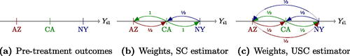
If CA is treated, the SC estimator puts equal weight on each of the equidistant control units. When either of the peripheral units, AZ or NY, is treated, the SC estimator puts all its weight on CA. The weights of the standard SC estimator are represented in Panel (b). The result is that in expectation CA is used as a control unit more than AZ or NY, and the total weight for CA as a control over all three assignments exceeds the weight CA gets as a treated unit. This difference in weights, or equivalently the imbalance of CA’s use as treatment and control unit, is what creates bias in the SC estimator under randomization. Adding a simple constraint to the weights which rules out this imbalance yields an unbiased Synthetic Control estimator. The resulting weights can be found in Panel (c). In this three-unit example, the unbiased SC estimator is simply the difference-in-means estimator, but with more than three units this is not generally true.

3.2 The Bias of the GSC Estimators

Having given a simple example of the bias of the SC estimator, we now study more broadly the bias of the four GSC estimators relative to the treatment effect for the treated unit, τ. We summarize the results in Table 3.

Table 3 Bias properties of GSC estimators for τ.

	Maintained assumptions
Randomization	Unit	Time	Time	Unit & time	Unit & time
			Large T		Large T
Assumptions	1	2	2, 3	1, 2	1, 2, 3
SC	Biased	Biased	Biased	Biased	Biased
MSC	Biased	Biased	Unbiased	Biased	Unbiased
USC	Unbiased	Biased	Biased	Unbiased	Unbiased
MUSC	Unbiased	Biased	Unbiased	Unbiased	Unbiased

Recall the general definition of the GSC estimators in (2.2), which can be rewritten as $$\begin{array}{c}\widehat{\tau }(\mathit{U},\mathit{V},\mathit{Y},\mathit{M})\\ =\sum _{t=1}^T\sum _{i=1}^N{V}_t{U}_i\left\{Y_{it}(1)+M_{i0t}+\sum _{j=1}^N(1-U_j)M_{\mathit{ijt}}{Y}_{jt}(0)\right\}.\end{array}$$

The estimation error relative to the treatment effect for the treated is equal to $$\begin{array}{c}\widehat{\tau }(\mathit{U},\mathit{V},\mathit{Y},\mathit{M})-\tau (\mathit{U},\mathit{V})\\ =\sum _{i=1}^N\sum _{t=1}^T{U}_i{V}_t\left\{Y_{it}(0)+M_{i0t}+\sum _{j=1}^N(1-U_j)M_{\mathit{ijt}}{Y}_{jt}(0)\right\}.\end{array}$$

We consider the bias of the GSC estimators separately for the estimators without an intercept (the SC and USC estimators), and for the estimators with the intercept (2.5) (the MSC and MUSC estimators).

Lemma 1.

Suppose Assumption 1 (random assignment of units to treatment) holds. If one of the following two conditions holds:

(i) the intercept is zero, $M_{i0t}=0$ for all i, t, or (ii) the intercept is not constrained and estimated through (2.5), then the conditional (on V) bias vanishes if the set of weights $\mathcal{M}$ imposes the condition that (3.1) $$\sum _{i=1}^N{M}_{\mathit{ijt}}=0\forall j=1,\dots ,N,t=1,\dots ,T.$$(3.1)

This lemma shows that ${\tau }^{\text{USC}}$ and ${\tau }^{\text{MUSC}}$ are unbiased, because both estimators only search over weight sets that satisfy the adding-up condition in (3.1). The above formulas also immediately lead to the bias of the SC estimator under Assumption 1.

Lemma 2.

Suppose Assumption 1 (random assignment of units to treatment) holds. Then conditional on V, the bias of the SC estimator is (3.2) $${\text{Bias}}^{\text{SC}}=\mathbb{E}\left[\widehat{\tau }-\tau |\mathit{V}\right]=\frac{1}{N}\sum _{j=1}^N\sum _{t=1}^T{V}_t{Y}_{jt}(0)\sum _{i=1}^N{M}_{\mathit{ijt}}^{\text{SC}}.$$(3.2)

The intuition for the bias of the SC estimator also holds for the simple matching estimator (e.g., Abadie and Imbens 2006), which is generally biased under randomization in finite samples.

In principle one can estimate the bias for the SC estimator in (3.2) and generate an unbiased estimator by subtracting the estimated bias from the standard SC estimator. However, in simulations, the bias estimates are very imprecise and as a result the properties of this de-biased estimator are not attractive in terms of RMSE.

To see the role that time randomization and the presence of an intercept play in the bias, consider the MSC estimator in a setting with large T and random selection of the treated period. For ease of exposition, suppose unit N is the treated unit. One can view the MSC estimator as a regression estimator where we regress the outcomes $Y_{N1},\dots ,Y_{NT}$ on the treatment indicator, the predictors $Y_{1,t},\dots ,Y_{N-1,t}$, and an intercept. It is well known that this leads to an estimator that is asymptotically unbiased in large samples (in this case meaning large T; see Freedman 2008; Lin 2013; Imbens and Rubin 2015).

A final comment concerns the magnitude of the bias. Although in our illustration the bias is small, it can in fact be arbitrarily large. Consider a case with binary outcomes, $Y_{it}(w)\in \{0,1\}$ and the treatment effect equal to zero for all units, $Y_{it}(0)=Y_{it}(1)$. Suppose the number of time periods is equal to the number of units. Moreover, suppose that for the first unit $Y_{1t}=0$ for $t=1,\dots ,T$. For all other units $i\ne 1$ $Y_{it}(0)=Y_{it}(1)=0$ for $t\notin \{i,T\}$ with $Y_{ii}(0)=Y_{ii}(1)=Y_{iT}(0)=Y_{iT}(1)=1$. In that case the first unit is matched with equal weight to all other units, $M_{\mathit{ijT}}=-1/(N-1)$ for j=$2,\dots ,N-1$, and all other units are matched to the first unit: $M_{i1T}=-1$ for $j=2,\dots ,N$. The bias in this case is $(N-2)/N$ which can be made arbitrarily close to the maximum possible value of 1.

3.3 The Exact GSC Variance and its Unbiased Estimation

Here we analyze the GSC estimator under unit randomization (Assumption 1) only, conditioning on the time treated. Alternatively, we could analyze the GSC estimator under time randomization only, or under both unit and time randomization, but those inferences may be less attractive in practice if only the last period is the treated period.

Lemma 3.

Suppose Assumption 1 holds. Then $$\begin{array}{c}\mathbb{V}(\mathit{V},\mathit{M})=\mathbb{E}\left[{\left(\widehat{\tau }(\mathit{U},\mathit{V},\mathit{Y},\mathit{M})-\tau \right)}^2|\mathit{V}\right]\\ =\frac{1}{N}\sum _{i=1}^N\sum _{t=1}^T{V}_t{\left(M_{i0t}+\sum _{j=1}^N{M}_{\mathit{ijt}}{Y}_{jt}(0)\right)}^2.\end{array}$$

For the unbiased estimators, this is the variance around the treatment effect τ on the treated unit, while for the other estimators, it is the expected squared error. The challenge is that the variance depends on control outcomes that we do not observe. However, we can estimate this variance without bias under unit randomization.

Proposition 1.

Suppose Assumption 1 holds. Then the estimator (3.3) $$\begin{array}{c}\widehat{\mathbb{V}}=\sum _{i=1}^N\sum _{t=1}^T{U}_i{V}_t\{\frac{1}{N-3}\sum _{\stackrel{k=1}{k\ne i}}^N{\left(\sum _{\stackrel{j=1}{j\ne i}}^N{M}_{\mathit{kjt}}(Y_{kt}-Y_{jt})\right)}^2\\ \hspace{1em}-\frac{1}{(N-2)(N-3)}\sum _{\stackrel{k=1}{k\ne i}}^N\sum _{\stackrel{j=1}{j\ne i}}^N{\mathit{M}}_{\mathit{kjt}}^2{(Y_{kt}-Y_{jt})}^2\\ \hspace{1em}+\frac{2}{N-2}\sum _{\stackrel{k=1}{k\ne i}}^N{M}_{k0t}\left(\sum _{\stackrel{j=1}{j\ne i}}^N{M}_{\mathit{kjt}}(Y_{jt}-Y_{kt})\right)+\frac{1}{N}\sum _{k=1}^N{\mathit{M}}_{k0t}^2\},\end{array}$$(3.3) is unbiased for $\mathbb{V}(\mathit{V},\mathit{M})$.

This result may be somewhat surprising. Note that in completely randomized experiments there is no unbiased estimator of the variance of the simple difference-in-means estimator for the average treatment effect (Imbens and Rubin 2015). The current result is different because here we focus on the effect for the treated only. For that estimand, there is an unbiased estimator for the variance of the difference-in-means estimator in the case of randomized experiments (e.g., Sekhon and Shem-Tov 2020).

The variance estimator in this proposition has three terms. The first takes the form of a leave-one-out estimator based on the control units excluding the treated unit. The remaining two terms correct for over-counting the diagonal elements in the inner square of the first term and additional terms for the intercept. In the special case of the DiM estimator, the variance reduces to the standard variance estimator. In that case, it is guaranteed to be nonnegative, which does not hold in general.

3.4 The Placebo Variance Estimator

To put the proposed variance estimator in (3.3) in perspective, we consider here an alternative approach for estimating the variance of the SC estimator. Versions of this placebo variance estimator have been proposed previously both for testing zero effects (e.g., Abadie, Diamond, and Hainmueller 2010) and for constructing confidence intervals (e.g., Doudchenko and Imbens 2016). Suppose unit i is the treated unit. We put this unit aside, and focus on the N – 1 control units. For each of these N – 1 control units (indexed by $j=1,\dots ,N,j\ne i$), we recalculate the weights, leaving out the treated unit, and then estimate the treatment effect. For ease of exposition we focus on the case where the last period is the treated period, V _T = 1.

We now define $(N-1)\times N$ weight matrices and sets of weight matrices ${\mathit{M}}^{(i)}$ and ${\mathcal{M}}^{(i)}$ from the restriction of M and $\mathcal{M}$ to units $j\ne i$. The weights are defined as (3.4) $${\mathit{M}}^{(i)}(\mathit{Y},{\mathcal{M}}^{(i)})=\underset{{\mathit{M}}^{(i)}\in {\mathcal{M}}^{(i)}}{\text{arg} \text{min}}\sum _{s=1}^{T-1}\sum _{\stackrel{j=1}{j\ne i}}^N{\left(M_{j0}^{(i)}+\sum _{\stackrel{k=1}{k\ne i}}^N{M}_{jk}^{(i)}{Y}_{ks}\right)}^2.$$(3.4)

Given these weights, the placebo estimator is $${\widehat{\tau }}_j^{(i)}=M_{j0}^{(i)}+\sum _{\stackrel{k=1}{k\ne i}}^N{M}_{jk}^{(i)}{Y}_{kT},\text{for}j\ne i.$$

Because unit j is a control unit, this is an estimator of zero, and the placebo variance estimator uses it to estimate the variance of $\widehat{\tau }$ as $$\begin{array}{c}{\widehat{\mathbb{V}}}^{\mathit{PCB}}=\frac{1}{N-1}\sum _{i=1}^N{U}_i\sum _{\stackrel{j=1}{j\ne i}}^N{\left({\widehat{\tau }}_j^{(i)}\right)}^2\\ =\frac{1}{N-1}\sum _{i=1}^N{U}_i\sum _{\stackrel{j=1}{j\ne i}}^N{\left(M_{j0}^{(i)}+\sum _{\stackrel{k=1}{k\ne i}}^N{M}_{jk}^{(i)}{Y}_{kT}\right)}^2.\end{array}$$

This variance estimator can be upward as well as downward biased, depending on the potential outcomes. In order to demonstrate this, we provide two toy examples in Appendix B where the placebo variance estimator is biased downward and upward, respectively.

3.5 Randomization Inference and Confidence Intervals

Within our design-based framework, a natural way of testing and providing confidence intervals is based on performing randomization inference directly, rather than relying solely on the estimated variance. In this section, we lay out how one can construct randomization-based tests and confidence intervals, building upon placebo tests for Synthetic Control in Abadie, Diamond, and Hainmueller (2010) and similar to Firpo and Possebom (2018). As in our related discussion of the placebo variance in the previous section, we focus on the case of unit randomization (Assumption 1) with treatment in the last period (V _T = 1). We note that the derivation applies to any GSC estimator, not just the specific USC and MUSC estimators.

We consider tests of the null hypothesis ${\tau }_i=Y_{iT}(1)-Y_{iT}(0)=\beta$, where i is the index of the treated unit. In our setting, for every unit j, ${\widehat{\tau }}_j-{\tau }_j=M_{j0T}+{\sum }_{k=1}^N{M}_{\mathit{jkT}}{Y}_{kT}(0)$ where ${\widehat{\tau }}_j$ is the GSC estimator of ${\tau }_j=Y_{jT}(1)-Y_{jT}(0)$. Under the null hypothesis, $Y_{jT}(0)=Y_{jT}-\beta \mathbb{1}\{j=i\}.$ That means that under the null $${\widehat{\tau }}_j-{\tau }_j=M_{j0T}+\sum _{k=1}^N{M}_{\mathit{jkT}}{Y}_{kT}-\beta M_{\mathit{jiT}}.$$

We consider a test based on quantiles of ${\widehat{\tau }}_j-{\tau }_j$. We have for $j\ne i$ that $$\begin{array}{c}{\widehat{\tau }}_j-{\tau }_j\ge {\widehat{\tau }}_i-{\tau }_i\\ \iff \beta (M_{\mathit{iiT}}-M_{\mathit{jiT}})+(M_{i0T}-M_{j0T})\\ +\sum _{k=1}^N(M_{\mathit{jkT}}-M_{\mathit{ikT}})Y_{kT}\ge 0\\ \iff \beta \ge \frac{M_{i0T}-M_{j0T}+\sum _{j=1}^N(M_{\mathit{ikT}}-M_{\mathit{jkT}})Y_{kT}}{M_{\mathit{iiT}}-M_{\mathit{jiT}}}={\widehat{\beta }}_j.\end{array}$$

We specifically construct a permutation test of size α for ${\widehat{\tau }}_j-{\tau }_j$. With a two-tailed test of size α, we would not reject $H_0:Y_{iT}(1)=Y_{iT}(0)+\beta$ whenever $q_{\alpha /2}({\sum }_{j=1}^N{U}_j({\widehat{\tau }}_j-{\tau }_j))<{\widehat{\tau }}_i-{\tau }_i\le q_{1-\alpha /2}({\sum }_{j=1}^N{U}_j({\widehat{\tau }}_j-{\tau }_j))$, which is equivalent to $$q_{\alpha /2}\left(\sum _{j=1}^N{U}_j{\widehat{\beta }}_j\right)<\beta \le q_{1-\alpha /2}\left(\sum _{j=1}^N{U}_j{\widehat{\beta }}_j\right),$$where we set ${\widehat{\beta }}_i=\beta$ and choose randomized quantiles to ensure exact size. This procedure yields a randomization test of H₀ that has exact size within our design-based framework. It differs from the test considered in Firpo and Possebom (2018), which is instead based on the fit of the Synthetic Control estimator and uses a weighted p-value to test null hypotheses about treatment effects.

We can then obtain confidence intervals based on test inversion, analogous to Firpo and Possebom (2018) but based on our specific unit permutation test of size α above for the treatment effect τ_i on unit i. Writing ${\widehat{\beta }}_{(1)},\dots ,{\widehat{\beta }}_{(N-1)}$ for the order statistics of ${\widehat{\beta }}_j$ with $j\ne i$, we obtain a $1-\alpha$ confidence interval $${\tau }_i\in \left[{\widehat{\beta }}_{(N\alpha /2)},{\widehat{\beta }}_{(N(1-\alpha /2))}\right]$$for the estimand τ_i, which is itself random. Here, we assume that a fractional order statistic ${\widehat{\beta }}_{(u)}$ with $u=\lfloor u\rfloor +\delta$ for $\delta \in [0,1)$ is equal to ${\widehat{\beta }}_{(\lfloor u\rfloor )}$ with probability $1-\delta$, and ${\widehat{\beta }}_{(\lfloor u\rfloor +1)}$ with probability δ. We could alternatively obtain confidence intervals that have potentially shorter length, for example, by inverting a test based on the quantiles of $|{\widehat{\tau }}_j-{\tau }_j|$.

3.6 Improvement over the Difference-in-Means Estimator

Simulations in Section 4.1 show that the variance of the MUSC and SC estimators can be substantially smaller than that of the DiM estimator. However, that is not guaranteed if we only make the assumption that the treated unit was randomly selected. It is possible that in the treated period the pattern between the outcomes is very different from that in the other periods, so that the MUSC and SC estimators have variances larger than that of the DiM estimator. However, this scenario can be ruled out if the treated time period is randomly selected among all periods (Assumption 2) and the number of time periods is large (Assumption 3):

Proposition 2.

Suppose Assumptions 1–3 hold. Let $\mathbb{V}(\mathcal{M})=\mathbb{E}\left[{(\widehat{\tau }-\tau )}^2\right]$ be the expected squared error of the GSC estimator $\widehat{\tau }$ with a time-invariant and convex constraint set $\mathcal{M}$, and let ${\mathbb{V}}^{\text{DiM}}$ be the variance of the corresponding DiM estimator. Suppose that the constraint set $\mathcal{M}$ allows for equal weights that sum to one (the DiM estimator). Then $$\underset{T\to \infty }{\text{lim}}\mathbb{V}(\mathcal{M})\le \underset{T\to \infty }{\text{lim}}{\mathbb{V}}^{\text{DiM}}.$$

An informal proof goes as follows. Writing $\mathcal{B}\subseteq {\mathbb{R}}^{N\times (N+1)}$ for the constraint set at a given time (so that $\mathcal{M}={\mathcal{B}}^T$), define $$\begin{array}{c}{\mathit{\beta }}_T^{*}=\underset{\mathit{\beta }\in \mathcal{B}}{\text{arg} \text{min}}\mathbb{E}[\sum _{i=1}^N\sum _{t=1}^T{U}_i{V}_t(Y_{it}(0)-{\beta }_{i0}\\ \mathrm{\hspace{1em}}\mathrm{\hspace{1em}}{-\sum _{j\ne i}{\beta }_{ij}{Y}_{jt}(0))}^2]\end{array}$$for the best set of GSC weights from $\mathcal{M}$ that are constant over time. First, since $\mathcal{M}$ contains the DiM estimator, ${\mathit{\beta }}_T^{*}$ has expected loss at most that of the DiM estimator. Second, the weights of the GSC estimator $\widehat{\tau }={\sum }_{i=1}^N{\sum }_{t=1}^T{U}_i{V}_t({\widehat{M}}_{i0t}+\sum _{j\ne i}{\widehat{M}}_{\mathit{ijt}}{Y}_{it})$ for large T and sufficiently large t approximate the oracle GSC weights ${\mathit{\beta }}_T^{*}$, and achieve similar loss in the limit. Note that this holds for the set of weights ${\mathcal{M}}^{\text{SC}}$, as well as for other GSC estimators. Chen (2022) generalizes this result and discusses the connection to online learning.

3.7 A Network Interpretation of SC Estimators and Their Bias

To understand the bias of SC estimators, we note that SC weights $$\begin{array}{c}\mathit{M}\in {\mathcal{M}}^{\text{SC}}=\{\mathit{M}|M_{\mathit{iit}}=1,\forall i,t;M_{\mathit{ijt}}\le 0,\forall i,j\ge 1,t;\\ \sum _{j=1}^N{M}_{\mathit{ijt}}=0\forall i,t;M_{i0t}=0\forall i\}\end{array}$$for a given treatment time t can be understood as a directed network with vertices i and edge flows (or weights) $W_{ij}=-M_{\mathit{jit}}\ge 0$ from vertex i to vertex $j\ne i$. The weight constraint ${\sum }_{j=1}^N{M}_{\mathit{ijt}}=0$ then ensures that the total incoming flow equals one for all vertices i, $\sum _{j\ne i}{W}_{ij}=1$. An example of such a network representation of an SC estimator is given in Figure 1(b).

Bias arises in the SC network whenever the incoming flow (which measures how often a unit is treated) is not the same as the outgoing flow of a vertex (which measures how often each unit is used as a control). The network corresponding to the SC estimator in Figure 1 is imbalanced: for the outside vertices, inflow exceeds outflow, while the inside vertex has higher outflow than inflow. Imposing the unbiasedness constraint ${\sum }_{j=1}^N{M}_{\mathit{jit}}=0$ is equivalent to imposing the flow balance constraint $\sum _{j\ne i}{W}_{ij}=\sum _{j\ne i}{W}_{ji}$ at all vertices i, ensuring that the corresponding units are used as often as controls as they are treated. Such a network is obtained in Figure 1(c), where inflows and outflows are balanced.

Beyond providing an intuitive language to represent Synthetic Control estimators, we show in Section 3.8 how tools from network analysis can help analyzing their properties. There, we show that the eigenvector centrality in the network represented by W relates to propensity scores subject to which an SC estimator is unbiased. With this network representation, we thus connect the SC estimator to the tools and insights from the literature on networks across statistics and the social sciences (e.g., Jackson 2010; de Paula 2020).

3.8 Nonconstant Propensity Scores

So far we have assumed that treatment is assigned with equal probability across units, time periods, or unit–time pairs. Yet the theory we develop generalizes to nonconstant propensity scores. See also Firpo and Possebom (2018) for extensions of SC placebo tests to nonconstant propensity scores. Here, we focus on the case where treatment happens at time t and is assigned randomly to single unit i with probability $p_i^{(t)}\in [0,1]$, where ${\sum }_{i=1}^N{p}_i^{(t)}=1$. We can also accomodate the setting where the set of possibe time periods at which treatment can occur is a proper subset of $\{1,\dots ,T\}.$ We ask whether an estimator ${\widehat{\tau }}^{\text{GSC}}(\mathit{U},\mathit{V},\mathit{Y},\mathit{M})\equiv {\sum }_{i=1}^N{\sum }_{t=1}^T{U}_i{V}_t\left\{M_{i0t}+{\sum }_{j=1}^N{M}_{\mathit{ijt}}{Y}_{jt}\right\}$ is unbiased for $\tau (\mathit{U},\mathit{V})={\sum }_{i=1}^N{\sum }_{t=1}^T{U}_i{V}_t{Y}_{it}(1)-Y_{it}(0)$ with respect to these propensity scores.

Proposition 3.

The estimator ${\widehat{\tau }}^{\text{GSC}}$ is unbiased for $\tau (\mathit{U},\mathit{V})$ (across values of potential outcomes) if and only if $\mathit{M}\in {\mathcal{M}}_p^{\text{MUSC}}=\left\{\mathit{M}|{\sum }_{j=1}^N{M}_{\mathit{ijt}}=0\forall i,t,{\sum }_{i=1}^N{p}_i^{(t)}{M}_{\mathit{ijt}}=0\forall j,t\right\}.$

Here, unbiasedness generalizes the adding-up condition ${\sum }_{i=1}^N{M}_{\mathit{ijt}}=0$ from the class of MUSC matrices to its propensity-weighted analogue ${\sum }_{i=1}^N{p}_i^{(t)}{M}_{\mathit{ijt}}=0$, which ensures that the bias is zero since $\mathbb{E}\left[\widehat{\tau }-\tau |\mathit{V}\right]={\sum }_{t=1}^T{V}_t$ $({\sum }_{i=1}^N{Y}_{it}(0){\sum }_{j=1}^N{p}_j^{(t)}{M}_{\mathit{jit}}+{\sum }_{j=1}^N{p}_j^{(t)}{M}_{j0t}).$A natural analogue of the MUSC estimator is then (3.5) $$\begin{array}{c}{\mathit{M}}_p^{\text{MUSC}}(\mathit{Y},{\mathcal{M}}_p^{\text{MUSC}})\equiv \underset{\mathit{M}\in {\mathcal{M}}_p^{\text{MUSC}}}{\text{arg} \text{min}}\sum _{i=1}^N{p}_i^{(t)}\\ \hspace{1em}\times \sum _{t=1}^T\left\{\sum _{s<t}{\left(M_{i0t}+\sum _{j=1}^N{M}_{\mathit{ijt}}{Y}_{js}\right)}^2\right\}.\end{array}$$(3.5)

Such an estimator could be used when treatment is assigned randomly. Note that the variance estimator from Proposition 1 extends. When the analyst has a choice over the treatment assignment, and t = T, the optimization in (3.5) could also include the choice of propensity score.

We now illustrate how varying propensity scores can affect the Synthetic Control estimator, extending the motivating example in Section 3.1. In this example, we consider the standard SC estimator, the USC estimator with equal propensities, and the USC estimator with non-constant propensities. Recall that the standard SC estimator is biased under this design and the USC estimator corrects this bias by enforcing balance between the probability of being treated and being used as a control. However, when the central unit is treated with higher probability of $\begin{array}{c}1/2\\ \end{array}$ (Figure 2(b)), then the weight matrix that only uses the closest units as control in each case is the optimal unbiased solution. In this specific example, this solution also coincides with the standard SC solution.

Fig. 2 Pre-treatment outcome in three-unit, two-period example with varying treatment propensities. An outgoing arrow represents the weight assigned to that unit when the target of the arrow is treated, and arrows are colored by the unit the respective weight is put on.

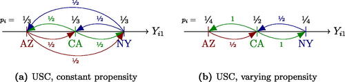
In this example, there is a set of propensity scores for which the standard SC estimator is unbiased. This is not a coincidence. As the following proposition shows, for the weights of every SC-type estimator there is a set of propensity scores such that the corresponding estimator is unbiased.

Proposition 4.

For every SC weight matrix $$\begin{array}{c}\mathit{M}\in {\mathcal{M}}^{\text{SC}}=\{\mathit{M}|M_{\mathit{iit}}=1,\forall i,t;M_{\mathit{ijt}}\le 0,\forall i,j\ge 1,\\ t;\sum _{j=1}^N{M}_{\mathit{ijt}}=0\forall i,t;M_{i0t}=0\forall i\}\end{array}$$there exists a propensity-score vector ${\mathit{p}}^{(t)}\in {[0,1]}^N,{\sum }_{i=1}^N{p}_i^{(t)}=1$ such that the corresponding estimator is unbiased with respect to ${\mathit{p}}^{(t)}$ at treatment time t.

This proposition does not rely on the weight matrix M being the result of a specific optimization program, as it applies to any weight matrix that follows the basic structure of the SC matrices (without intercept).

To understand the propensity scores ${\mathit{p}}^{(t)}$ that make the SC estimator associated with the weights M unbiased, we note that they can be interpreted as a measure of centrality in the network associated with M in a precise way, where more central units correspond to higher propensity scores. Specifically, let $\mathit{W}={(W_{ij})}_{i,j\in \{1,\dots ,N\}}$ be the edge flow matrix from Section 3.7 corresponding to M for treatment time t, meaning that $W_{ij}=-M_{\mathit{jit}}$ for $i\ne j$ and W_ii = 0. Then the eigenvector centralities of vertices in this network are equivalent (up to normalization) to the propensity scores that ensure unbiasedness, where we consider the case where both are unique.

Proposition 5.

Assume that the network W associated with M for treatment at t is strongly connected (equivalently, that W is irreducible). Then the propensity score vector ${\mathit{p}}^{(t)}$ for which the estimator is unbiased at t is unique and the same as the eigenvector centrality in the network W (with appropriate normalization).

This connection between eigenvectors and unbiased propensities follows naturally from the representation of the estimator in terms of its (weighted) network adjacency matrix W. Writing ${\mathit{M}}^{(t)}={(M_{\mathit{ijt}})}_{i,j\in \{1,\dots ,N\}}$ for the N × N matrix corresponding to the SC weights when treatment happens at t, the unbiasedness condition corresponds to $({\mathit{M}}^{(t)})\prime {\mathit{p}}^{(t)}=\mathbf{0}$. Since $({\mathit{M}}^{(t)})\prime =\mathbb{I}-\mathit{W}$, ${\mathit{p}}^{(t)}$ is an eigenvector of W with eigenvalue 1, which is also the largest eigenvalue and corresponds to the unique nonnegative eigenvector if the network is strongly connected. When the network is not strongly connected, we may still obtain a similar result for its components.

These results suggest ways in which considering varying propensity scores can be helpful when analyzing SC-type estimators. First, when treatment is randomized according to a known probability distribution, then those probabilities affect the optimal USC and MUSC weights. Second, the propensities that make an estimator unbiased have an intuitive interpretation as the eigenvector centralities of the network corresponding to the weight matrix of an SC estimator. Third, even in the observational case, varying propensities could be used when some units can be considered to be more likely to receive treatment or to be more appropriate as controls, replacing binary inclusion criteria by treatment propensities. Finally, when we choose propensity scores in the design of an experiment and plan to use an SC-type estimator, we can optimize the choice of propensities based on past outcomes to be better suited to their relationship, assigning more central units higher probabilities.

4 An Illustration and Some Simulations

In this section we illustrate some of the methods proposed in the first part of this article. We first report the results of a simulation study based on real data. Second, we report results of a re-analysis of the California smoking study (Abadie, Diamond, and Hainmueller 2010).

4.1 A Simulation Study

We perform a small simulation study to assess the properties of the MUSC estimator. Following Bertrand, Duflo, and Mullainathan (2004) and Arkhangelsky et al. (2019), we use data from the Current Population Survey for N = 50 states and T = 40 years. The variables we analyze include state/year average log wages, hours, and the state/year unemployment rate. The true treatment effects are all zero by construction. This allows us to calculate the RMSE. For each of the variables, we estimate the treatment effects using the Difference-in-Means (DiM) estimator, the standard Synthetic Control (SC) estimator, the Difference-in-Differences (DiD) estimator, and the Modified Unbiased Synthetic Control (MUSC) estimator. We also include for comparison the LASSO estimator based on regressing the period T outcomes on all the lagged outcomes. The LASSO estimator is not an SC-type estimator and is generally biased in our framework, and we merely include it as a benchmark that uses more information than the DiM estimator. For the LASSO estimator, we choose the regularization parameter using leave-one-out cross validation.

The first simulation study we conduct compares the performance of the six estimators in terms of RMSE. The study is designed as follows. For each treated period $T\in \{21,\dots ,40\}$, we use T – 1 pretreatment periods to estimate weights for the six estimators and discard all data after T. Then, iterating through all 50 states, we pretend that each state has been selected for treatment and calculate the corresponding estimated treatment effects. Lastly, we average over all states to summarize the performance for a single treated period.

In Table 4, we report the results averaged over all 20 years. We report the results for the setting with 50 units, as well as for settings with 10 and 5 units to assess the relative performance with fewer cross-sectional units. We find that the RMSE is substantially lower for the SC and MUSC estimator compared to the DiM estimator for all variables. In Table 1 in the appendix, we document that these results hold across years. The SC and MUSC estimators perform comparably to the LASSO estimator for log wages and outperform it for the other two variables in the case with N = 50, with the DiD estimator performing worse than any of these three. Note that the SC and MUSC estimators have similar RMSE in this case. In the cases with N = 10 and N = 5, the MUSC estimator substantially outperforms the other methods except for the DiD estimator, with the latter performing slightly worse for N = 10 and slightly better for N = 5. Overall, the MUSC estimator performs consistently well. Unsurprisingly the relative performance of the LASSO estimator deteriorates sharply when the number of units is small and there are not enough control units to estimate the LASSO parameters well. Additional simulations show that the DiD estimator performs relatively poorly when many of the units are well approximated by a small number of control units.

Table 4 Simulation experiment based on CPS data averaged over states and years—root-mean-squared-error (RMSE).

	N = 50			N = 10			N = 5
Est	Ln(Wage)	Hours	U-Rate	Ln(Wage)	Hours	U-Rate	Ln(Wage)	Hours	U-Rate
DiM	0.105	1.197	0.015	0.122	1.558	0.016	0.144	1.380	0.015
SC	0.051	0.918	0.013	0.070	1.045	0.015	0.079	1.010	0.014
SC–NR	0.076	1.350	0.019	0.064	1.049	0.017	0.058	0.965	0.013
MUSC	0.053	0.903	0.013	0.061	0.960	0.015	0.057	0.944	0.013
LASSO	0.051	0.952	0.013	0.077	1.313	0.017	0.116	1.251	0.015
DiD	0.063	0.976	0.013	0.066	0.982	0.014	0.055	0.929	0.013

DiM: Difference-in-Means estimator, SC: Synthetic Control estimator of Abadie, Diamond, and Hainmueller (2010), SC–NR: Synthetic Control Estimator with no adding up restriction on the weights, MUSC: Modified Unbiased Synthetic Control estimator, DiD: Difference-in-Differences estimator.

The second simulation study demonstrates the properties of our proposed unbiased variance estimator and the placebo variance estimator. Here we focus on average log wages and fix T = 40 as the treated period. Moreover, we decrease the sample to N = 20 units in total. Table 5 reports standard errors based on the true variance along with the estimates (averaged over all units) based on our variance estimator and using the placebo approach. We find that our estimator is indeed unbiased. The placebo approach is very modestly biased—the direction of the bias depends on which estimator is used. For the DiM, the DiD, and the SC estimator, the placebo estimator is upward biased; for the MUSC estimator it is downward biased.

Table 5 Simulation experiment based on CPS data (log wages) by state and year for N = 20 units and treated period T = 40 – average standard error.

	$\sqrt{V_{\text{true}}}$	$\sqrt{{\widehat{V}}_{\text{GSC}}}$	$\sqrt{{\widehat{V}}_{\text{PCB}}}$
DiM	0.1157	0.1157	0.1158
SC	0.0518	0.0518	0.0521
MUSC	0.0490	0.0490	0.0489
DiD	0.0553	0.0553	0.0554

DiM: Difference in Means, SC: Synthetic Control, MUSC: Modified Synthetic Control, DiD: Difference in Differences, GSC: General Synthetic Control, PCB: Placebo

A third simulation exercise study illustrates the coverage and length of randomization-based confidence intervals as well as confidence intervals based on Normal-distribution approximation using our unbiased variance estimate. We discuss the construction of the randomization based confidence intervals in Section 3.5. Table 6 shows the results. We find that our randomization-based confidence intervals provide correct coverage, while Normality-based intervals may under- or over-cover. This is unsurprising because they are not formally justified in the case with a single treated unit/time period combination, which we focus on in this article.

Table 6 Confidence intervals.

		Randomization-based		Normality-based
Variable	Estimator	Coverage	Length	Coverage	Length
Urate	DiM	0.950	0.061	0.947	0.059
	SC	0.950	0.055	0.944	0.051
	MUSC	0.950	0.056	0.945	0.051
Hours	DiM	0.950	5.051	0.943	4.693
	SC	0.950	3.905	0.951	3.597
	MUSC	0.950	3.996	0.939	3.539
Lwage	DiM	0.950	0.429	0.951	0.410
	SC	0.950	0.219	0.939	0.200
	MUSC	0.950	0.238	0.945	0.207

NOTE: Coverage and length of confidence intervals based on the MUSC estimator and, in the case of Normality-based intervals, our unbiased estimator of its variance. Coverage and length is averaged over 5000 random draws of the treated unit and period from $T=21\dots 40$, S = 5000.

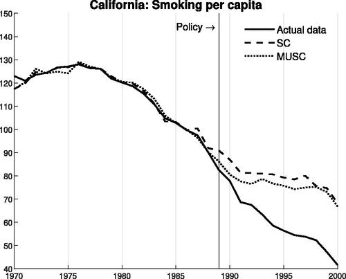
4.2 The California Smoking Study

Next, we turn to the data from the California smoking study (Abadie, Diamond, and Hainmueller 2010). In Figure 3 we compare the SC and MUSC estimates. We find that the pretreatment fit is similar for both estimators despite the additional restriction. In addition, the point estimates are similar. The interpretation is that the number of “similar” control units is large enough that a single additional restriction (and the relaxing of another one) does not affect the goodness of fit substantially.

Fig. 3 Pre- and post-treatment fit of SC and MUSC.

5 Conclusion

In this article, we study Synthetic Control (SC) methods from a design perspective. We show that when a randomized experiment is conducted, the standard SC estimator is biased. However, a minor modification of the SC estimator is unbiased under randomization, and in cases with few treated units can have RMSE properties superior to those of the standard Difference-in-Means estimator. We show that the design perspective also has implications for observational studies. We propose a variance estimator validated by randomization.

In the online appendix we discuss some extensions, including the results for the case with multiple treated units in Appendix D.1 and the case where the estimand is the average effect for all units in the treated period, ${\tau }^{\text{V}}$, in Appendix D.2.

Supplementary Materials

Supplementary materials are four appendices. Appendix A: Additional table. Appendix B: Additional theoretical results. Appendix C: Proofs. Appendix D: Extensions and Generalizations.

Acknowledgments

The authors would like to thank Alberto Abadie, Kirill Borusyak, Jonathan Roth, Jeffrey Wooldridge, the editor, the associate editor, three anonymous referees, and seminar audiences at the NBER and at USC for helpful comments and general discussions on the topic of this article.

Disclosure Statement

No potential conflict of interest was reported by the authors.

Additional information

Funding

This research was generously supported by ONR grants N00014-17-1-2131 and N00014-19-1-2468 and a gift from Amazon.

References

- Abadie, A. (2021), “Using Synthetic Controls: Feasibility, Data Requirements, and Methodological Aspects,” Journal of Economic Literature, 59, 391–425. DOI: 10.1257/jel.20191450.
- Abadie, A., Athey, S., Imbens, G. W., and Wooldridge, J. M. (2020), “Sampling-based versus Design-based Uncertainty in Regression Analysis,” Econometrica, 88, 265–296. DOI: 10.3982/ECTA12675.
- Abadie, A., Diamond, A., and Hainmueller, J. (2010), “Synthetic Control Methods for Comparative Case Studies: Estimating the Effect of California’s Tobacco Control Program,” Journal of the American statistical Association, 105, 493–505. DOI: 10.1198/jasa.2009.ap08746.
- Abadie, A., Diamond, A., and Hainmueller, J. (2015), “Comparative Politics and the Synthetic Control Method,” American Journal of Political Science, 59, 495–510.
- Abadie, A., and Gardeazabal, J. (2003), “The Economic Costs of Conflict: A Case Study of the Basque Country,” American Economic Review, 93, 113–132. DOI: 10.1257/000282803321455188.
- Abadie, A., and Imbens, G. W. (2006), “Large Sample Properties of Matching Estimators for Average Treatment Effects,” Econometrica, 74, 235–267. DOI: 10.1111/j.1468-0262.2006.00655.x.
- Abadie, A., and L’Hour, J. (2017), “A Penalized Synthetic Control Estimator for Disaggregated Data,” Working Papers, Massachusetts Institute of Technology, Cambridge, MA.
- Abadie, A., and Zhao, J. (2021), “Synthetic Controls for Experimental Design,” arXiv preprint arXiv:2108.02196.
- Amjad, M., Shah, D., and Shen, D. (2018), “Robust Synthetic Control,” The Journal of Machine Learning Research, 19, 802–852.
- Arkhangelsky, D., Athey, S., Hirshberg, D. A., Imbens, G. W., and Wager, S. (2019), “Synthetic Difference in Differences,” Technical Report, National Bureau of Economic Research.
- Athey, S., Bayati, M., Doudchenko, N., Imbens, G., and Khosravi, K. (2021). Matrix completion methods for causal panel data models. Journal of the American Statistical Association. DOI: 10.1080/01621459.2021.1891924.
- Athey, S., and Imbens, G. W. (2018), “Design-based Analysis in Difference-in-Differences Settings with Staggered Adoption,” Technical report, National Bureau of Economic Research.
- Ben-Michael, E., Feller, A., and Rothstein, J. (2020), “The Augmented Synthetic Control Method,” arXiv preprint arXiv:1811.04170.
- Bertrand, M., Duflo, E., and Mullainathan, S. (2004), “How Much Should We Trust Differences-in-Differences Estimates?” The Quarterly Journal of Economics, 119, 249–275. DOI: 10.1162/003355304772839588.
- Cavallo, E., Galiani, S., Noy, I., and Pantano, J. (2013), “Catastrophic Natural Disasters and Economic Growth,” Review of Economics and Statistics, 95, 1549–1561. DOI: 10.1162/REST_a_00413.
- Chen, J. (2022), “Synthetic Control as Online Linear Regression,” arXiv preprint arXiv:2202.08426.
- Chernozhukov, V., Wuthrich, K., and Zhu, Y. (2017), “An Exact and Robust Conformal Inference Method for Counterfactual and Synthetic Controls,” arXiv preprint arXiv:1712.09089.
- Coffman, M., and Noy, I. (2012), “Hurricane Iniki: Measuring the Long-Term Economic Impact of a Natural Disaster Using Synthetic Control,” Environment and Development Economics, 17, 187–205. DOI: 10.1017/S1355770X11000350.
- Cunningham, S. (2018), Causal Inference: The Mixtape, London: Yale University Press.
- de Paula, Á. (2020), “Econometric Models of Network Formation,” Annual Review of Economics, 12, 775–799. DOI: 10.1146/annurev-economics-093019-113859.
- Doudchenko, N., and Imbens, G. W. (2016), “Balancing, Regression, Difference-in-Differences and Synthetic Control Methods: A Synthesis,” Technical Report, NBER.
- Ferman, B., and Pinto, C. (2017), “Placebo Tests for Synthetic Controls,” MPRA Paper 78079.
- Ferman, B., and Pinto, C. (2019), “Synthetic Controls with Imperfect Pre-treatment Fit,” arXiv preprint arXiv:1911.08521.
- Firpo, S., and Possebom, V. (2018), “Synthetic Control Method: Inference, Sensitivity Analysis and Confidence Sets,” Journal of Causal Inference, 6. DOI: 10.1515/jci-2016-0026.
- Fisher, R. A. (1937), The Design of Experiments, pp. 1–26, Edinburgh; London: Oliver and Boyd.
- Freedman, D. A. (2008), “On Regression Adjustments in Experiments with Several Treatments,” The Annals of Applied Statistics, 2, 176–196. DOI: 10.1214/07-AOAS143.
- Hahn, J., and Shi, R. (2016), “Synthetic Control and Inference,” Available at UCLA.
- Imbens, G. W., and Rubin, D. B. (2015), Causal Inference in Statistics, Social, and Biomedical Sciences, Cambridge: Cambridge University Press.
- Jackson, M. O. (2010), Social and Economic Networks, Princeton: Princeton University Press.
- Lei, L., and Candès, E. J. (2020), “Conformal Inference of Counterfactuals and Individual Treatment Effects,” arXiv preprint arXiv:2006.06138.
- Li, K. T. (2020), “Statistical Inference for Average Treatment Effects Estimated by Synthetic Control Methods,” Journal of the American Statistical Association, 115, 2068–2083. DOI: 10.1080/01621459.2019.1686986.
- Lin, W. (2013), “Agnostic Notes on Regression Adjustments for Experimental Data: Reexamining Freedman’s Critique,” The Annals of Applied Statistics, 7, 295–318. DOI: 10.1214/12-AOAS583.
- Liu, S. (2015), “Spillovers from Universities: Evidence from the Land-Grant Program,” Journal of Urban Economics, 87, 25–41. DOI: 10.1016/j.jue.2015.03.001.
- Manski, C. F., and Pepper, J. V. (2018), “How do Right-to-Carry Laws Affect Crime Rates? Coping with Ambiguity Using Bounded-Variation Assumptions,” Review of Economics and Statistics, 100, 232–244. DOI: 10.1162/REST_a_00689.
- Neyman, J. (1923/1990), “On the Application of Probability Theory to Agricultural Experiments. Essay on Principles. Section 9,” Statistical Science, 5, 465–472.
- Rambachan, A., and Roth, J. (2020), “Design-Based Uncertainty for Quasi-Experiments,” arXiv preprint arXiv:2008.00602.
- Rosenbaum, P. R. (2002), Observational Studies, New York: Springer.
- Roth, J., and Sant’Anna, P. H. (2021), “Efficient Estimation for Staggered Rollout Designs,” arXiv preprint arXiv:2102.01291.
- Rubin, D. B. (1974), “Estimating Causal Effects of Treatments in Randomized and Nonrandomized Studies,” Journal of Educational Psychology, 66, 688–701. DOI: 10.1037/h0037350.
- Rubin, D. B. (2008), “For Objective Causal Inference, Design Trumps Analysis,” The Annals of Applied Statistics, 2, 808–840.
- Sekhon, J. S., and Shem-Tov, Y. (2020), “Inference on a New Class of Sample Average Treatment Effects,” Journal of the American Statistical Association, 116, 798–804. DOI: 10.1080/01621459.2020.1730854.
- Xu, Y. (2017), “Generalized Synthetic Control Method: Causal Inference with Interactive Fixed Effects Models,” Political Analysis, 25, 57–76. DOI: 10.1017/pan.2016.2.