Modeling Extreme Events: Time-Varying Extreme Tail Shape

Abstract

We propose a dynamic semiparametric framework to study time variation in tail parameters. The framework builds on the Generalized Pareto Distribution (GPD) for modeling peaks over thresholds as in Extreme Value Theory, but casts the model in a conditional framework to allow for time-variation in the tail parameters. We establish parameter regions for stationarity and ergodicity and for the existence of (unconditional) moments and consider conditions for consistency and asymptotic normality of the maximum likelihood estimator for the deterministic parameters in the model. Two empirical datasets illustrate the usefulness of the approach: daily U.S. equity returns, and 15-min euro area sovereign bond yield changes.

Keywords:

• Dynamic tail risk
• Extreme value theory
• Observation-driven models
• Securities Markets Programme (SMP)
• Stock return tails

1 Introduction

This article proposes a dynamic semiparametric framework to study time variation in tail fatness for long univariate time series. The new method builds on ideas from Extreme Value Theory (EVT) and uses a conditional Generalized Pareto Distribution (GPD) with time-varying parameters to approximate the tail beyond a given threshold. The GPD is an appropriate tail approximation for most heavy-tailed densities used in financial economics, econometrics, and actuarial sciences; see, for example, Embrechts, Klüppelberg, and Mikosch (1997), Coles (2001), McNeil, Frey, and Embrechts (2010, chap. 7), and Rocco (2014). As a result, the GPD plays a central role in the study of extremes, comparable to the role of the normal distribution when studying observations in the center of the distribution. Our framework allows for studying time-variation in the incidence of such extremes.

The time-varying tail shape and tail scale parameters in our model are driven by the score of the GPD density; see Creal, Koopman, and Lucas (2013) and Harvey (2013). As a result, the model is observation-driven in the terminology of Cox (1981) and its time-varying parameters are perfectly predictable one step ahead. In addition, the log-likelihood function is known in closed form and allows for parameter estimation and inference via standard maximum likelihood methods. Our results show that our model is able to recover the time-varying tail shape and tail scale parameters well in both simulated and empirical data. In addition, the model recovers time-variation in EVT-based market risk measures such as Value-at-Risk (VaR) and Expected Shortfall (ES). This is the case even if the model is misspecified or the GPD approximation is not exact. The latter is particularly important in our finite sample setting, where the limiting EVT result of the GPD can only hold approximately given the choice of a finite exceedance threshold in any particular dataset.

We illustrate our modeling framework using two applications: U.S. equity log-returns, and changes in euro area sovereign bond yields.¹ Each dataset consists of two time series that we model separately. We first consider daily log-returns for a stock index (S&P500) and an individual stock (IBM). The S&P500 log-returns range from July 3, 1962 to December 31, 2020, while the IBM stock returns range from January 2, 1926 to December 31, 2020. Focusing on the left tail, and controlling for potential time-variation in the EVT thresholds, we find that both GPD parameters vary significantly over time. The tail shape varies between approximately 0.05 and 0.25 for the S&P 500, and between 0.05 and 0.35 for IBM. These values imply a maximum moment of order $1/0.25=4$ to $1/0.05=20$ for the S&P 500, and 3 to 20 for IBM. Confidence bands around the filtered time-varying tail shape parameters suggest that the tail shape parameter is almost always far from the thin-tailed setting.

Our second illustration demonstrates how additional control variables can be included to capture time-variation in tail shapes and tail scales. Specifically, we study changes in Italian and Portuguese five-year benchmark bond yields, sampled at a 15-min frequency, during the extremely adverse euro area sovereign debt crisis between 2010 and 2012. Again, we find that both GPD parameters vary significantly over time. The tail shape varies between 0.1 and 0.4 for Italy and between 0.05 and 0.6 for Portugal, implying moment ranges of 2.5–10 and 1.7–20, respectively, and thus incidences of extreme fat tails. We also find that part of the variation can be explained by including central bank bond purchases as an additional covariate, and provide a way to translate the estimated impact coefficients into their economically-interpretable impact on market risk measures such as VaR.

Our article is closely related to a growing strand of literature on modeling time-variation in EVT tail parameters. Several papers propose methodology to study time variation in the tail index. Davidson and Smith (1990), (Coles, 2001, chap. 5.3), and Wang and Tsai (2009), among others, also index the GPD tail parameters with time subscripts and equip them with a parameterized structure. Our approach is different in that their “tail index regression” approach requires conditioning variables that explain (all of) the tail variation. Such variables are not always available. By contrast, our “filtering approach” does not require such conditioning variables, and is arguably better suited for the real-time monitoring of extreme equity or bond market risks. Second, Quintos, Fan, and Phillips (2001), Einmahl, de Haan, and Zhou (2016), Hoga (2017), and Lin and Kao (2018) derive formal tests for a structural break in the tail index. A number of subsequent studies applied such tests to financial time series data. Werner and Upper (2004) identify a break in the tail behavior of high-frequency German Bund future returns. Galbraith and Zernov (2004) argues that certain regulatory changes in U.S. equity markets have altered the tail index dynamics of equities returns. de Haan and Zhou (2021) propose a nonparametric approach to estimating the extreme value index locally. Our article adds to the literature by proposing a framework that allows us to study both the tail shape and tail scale dynamics directly in a semiparametric way. Explanatory covariates can be included in the dynamics of both parameters, and likelihood ratio tests are available to test economically relevant hypotheses. Finally, unlike Patton, Ziegel, and Chen (2019), our tail VaR and ES dynamics explicitly account for fat tail shape beyond a threshold as emerging from EVT. The dynamics based on the score for the GPD contain weights for extreme observations. Such weights are absent in the elicitable score functions of Patton, Ziegel, and Chen (2019). The resulting dynamics in our model are more robust, particularly for the ES.

Whereas de Haan and Zhou (2021) take a nonparametric perspective, the methodological part of this article is closest to Massacci (2017), who also proposes a dynamic parametric model for the GPD parameters. Our framework is different from Massacci (2017) in that we specify both GPD parameters as functions of their respective scores. Massacci (2017), by contrast, uses only the score of the first (tail index) parameter to drive both parameters. This is not optimal in the sense of Blasques, Koopman, and Lucas (2015), who require that each time-varying parameter is associated to its own score. Our article further differs from Massacci (2017) in that we suggest time-varying EVT thresholds to locate the boundary between the center of the distribution and its tail. This implies that we do not need to assume that the time series at hand has no volatility clustering, nor that we need to pre-filter for such volatility clustering. Absence of conditional heteroscedasticity would be hard to defend for the financial data considered in this article. Finally, we differ from Massacci (2017) in that we discuss inference on both deterministic and time-varying parameters by considering the asymptotic properties of the maximum likelihood estimator, provide sufficient conditions for the stationarity and ergodicity and the existence of moments of the factor process and observations, explain how to introduce additional conditioning variables into the model and assess their usefulness in economic terms, and provide Monte Carlo evidence on the model’s performance in a range of challenging settings.

We proceed as follows. Section 2 presents our statistical model, the asymptotic statistical properties of the model and the maximum likelihood estimator. Section 3 discusses simulation results. Section 4 illustrates the model using U.S. equity data and euro area sovereign yields data. Section 5 concludes. Derivations and more results are in the web appendix.

2 Statistical Model

2.1 Time-Varying Tail Shape and Tail Scale

2.1.1 Conditional EVT Framework

Consider a univariate time series y_t, $t=1,\dots ,T$, where T denotes the number of observations. This section then describes our model for y_t with time-varying tail shape and scale. We assume y_t is generated by a conditional probability density function (pdf) $g(y_t | {\mathcal{F}}_{t-1})$, where ${\mathcal{F}}_{t-1} = \{y_{t-1},y_{t-2},\dots ,y_1\}$ denotes the information set containing all past data. By keeping the conditional density of y_t in its current general form, we stay close to the semiparametric nature of an extreme value-based approach and make no modeling assumptions about the center of the distribution. Alternatively, we could specify a parametric distribution for y_t with for instance a time-varying conditional location μ_t and scale σ_t. The μ_t and σ_t could then be used to pre-filter the raw y_t. We do not pursue such an approach here. First, modeling the center of the conditional distribution leads away from the focus on the tails only, which is the key aspect in an EVT-based approach. Second, designing an additional model for time-varying location and scale would create another layer of complexity to the model, with accompanying model risk and parameter uncertainty. We therefore keep the general form of $g(y_t | {\mathcal{F}}_{t-1})$ and focus on its tail using a dynamic extension of arguments from extreme value theory (EVT), similar to Patton’s (2006) extension of copula theory to the dynamic, observation driven setting.

We assume $g(y_t | {\mathcal{F}}_{t-1})$ has heavy tails with time-varying tail index ${\alpha }_t>0$. A familiar example is when $g(y_t | {\mathcal{F}}_{t-1})$ is a univariate Student’s t distribution with ${\nu }_t = {\alpha }_t$ degrees of freedom. Other examples include the Pareto, inverse gamma, log-gamma, log-logistic, F, Fréchet, and Burr distribution with one or more time-varying shape parameters (for details and further discussion see e.g., Johnson, Kotz, and Balakrishnan, 1994; Embrechts, Klüppelberg, and Mikosch, 1997; McNeil, Frey, and Embrechts, 2010, chap. 7.3). Rather than modeling the (dynamic) tail shape of an arbitrarily chosen parametric family of distributions, we appeal to well-known results from the EVT literature: the conditional cumulative distribution function (cdf) $G(y_t|{\mathcal{F}}_{t-1})$ of y_t can under very general conditions be approximated by $G(y_t|{\mathcal{F}}_{t-1})\approx G({\tau }_t|{\mathcal{F}}_{t-1})+(1-G({\tau }_t|{\mathcal{F}}_{t-1}))P(x_t;{\delta }_t,{\xi }_t)$ with $x_t=y_t-{\tau }_t$ for sufficiently high thresholds ${\tau }_t\in {\mathbb{R}}_{+}$. More precisely, we have (1) $$\begin{array}{c}\underset{{\tau }_t\to \infty }{\lim }\underset{x_t\ge 0}{\sup }| \mathbb{P}\left[Y_t\le x_t+{\tau }_t\left|\mathit{dle}\right|Y_t>{\tau }_t,{\mathcal{F}}_{t-1}\right]-P(x_t;{\delta }_t,{\xi }_t) |\\ =\underset{{\tau }_t\to \infty }{\lim }\underset{x_t\ge 0}{\sup }|\frac{G(x_t+{\tau }_t|{\mathcal{F}}_{t-1})-G({\tau }_t|{\mathcal{F}}_{t-1})}{1-G({\tau }_t|{\mathcal{F}}_{t-1})}\\ -P(x_t;{\delta }_t,{\xi }_t)|=0,\end{array}$$(1) for parameters ${\xi }_t={\alpha }_t^{-1}$ and δ_t, both possibly depending on τ_t, and with Y_t denoting the random variable corresponding to the realization y_t. Here, $P(x_t;{\delta }_t,{\xi }_t)$ denotes the cdf of the Generalized Pareto Distribution (GPD), with cdf and pdf given by (2) $$P(x_t;{\delta }_t,{\xi }_t)=1-{\left(1+{\xi }_t\frac{x_t}{{\delta }_t}\right)}^{-{\xi }_t^{-1}},$$(2) (3) $$p(x_t;{\delta }_t,{\xi }_t)={\delta }_t^{-1}·{\left(1+{\xi }_t\frac{x_t}{{\delta }_t}\right)}^{-{\xi }_t^{-1}-1},$$(3) respectively (see, e.g., McNeil, Frey, and Embrechts, 2010). The quantity $x_t=y_t-{\tau }_t>0$ is the so-called peak-over-threshold (POT), or exceedance, of heavy-tailed data y_t over a pre-determined threshold τ_t, and ${\delta }_t>0$ and ${\xi }_t>0$ are the tail scale and tail shape parameter of the GPD, respectively. Most continuous distributions used in statistics and the actuarial sciences lie in the Maximum Domain of Attraction (MDA) of the GPD (see McNeil, Frey, and Embrechts, 2010, chap. 7.1), meaning that they allow for the above tail shape approximation. By focusing on the tail area directly using EVT arguments, we avoid having to make more ad-hoc assumptions on the parametric form of the tail.

The result in (1) is a limiting result. In any finite sample, the threshold τ_t has to be set to a specific, finite value, such that the GPD approximation will be inexact and the distribution is in that sense misspecified. This will also be the case in our setting. The score-driven updates that we define later on for ξ_t and δ_t, however, still ensure that the expected Kullback-Leibler divergence between the approximate GPD model and the true, unknown conditional distribution $\mathbb{P}\left[Y_t\le x_t+{\tau }_t\left|\mathit{dle}\right|Y_t>{\tau }_t,{\mathcal{F}}_{t-1}\right]$ is improved on average at every step for sufficiently small steps, even if the GPD model is (partially) misspecified; see Blasques, Koopman, and Lucas (2015).

The choice of the threshold τ_t is subject to a well-known bias-variance tradeoff; see, for instance, McNeil and Frey (2000). In theory, the GPD tail approximation only becomes exact for ${\tau }_t\to +\infty$. A high threshold, however, also implies a smaller number of exceedances $y_t>{\tau }_t$, and more estimation error for the parameters of the GPD. Common choices for τ_t from the literature are the unconditional 90%, 95%, and 99% empirical quantiles of y_t; see Chavez-Demoulin, Embrechts, and Sardy (2014). In our setting, such choices are less useful as τ_t varies over time. As we explain later, we use the approach of Patton, Ziegel, and Chen (2019) to set τ_t dynamically in line with the data.

2.1.2 Time-Varying Parameters

A key step in (1)–(2) is that we use the conditional probabilities based on the information set ${\mathcal{F}}_{t-1}$. As a result, the tail parameters ξ_t and δ_t become time-varying. To capture this time-variation, we model $({\xi }_t,{\delta }_t)\prime$ using the score-driven dynamics introduced by Creal, Koopman, and Lucas (2013) and Harvey (2013). In our time series setting, this implies that both δ_t and ξ_t are measurable with respect to ${\mathcal{F}}_{t-1}$. We ensure positivity of δ_t and ξ_t by using an (element-wise) exponential link function $({\xi }_t,{\delta }_t)\prime =\hspace{0.17em}\exp \hspace{0.17em}(f_t)$ for $f_t=(f_t^{\xi },f_t^{\delta })\prime \in {\mathbb{R}}^2$. The transition dynamics for f_t are given by (4) $$\begin{array}{c}{f}_{t+1}=\omega +\sum _{i=0}^{q-1}{A}_i{s}_{t-i}+\sum _{j=0}^{p-1}{B}_j{f}_{t-j},\\ s_t={\mathcal{S}}_t{\nabla }_t,\mathrm{\hspace{1em}}\mathrm{\hspace{1em}}{\nabla }_t=\partial \hspace{0.17em}\ln \hspace{0.17em}p(x_t|{\mathcal{F}}_{t-1};f_t,\theta )/\partial f_t,\end{array}$$(4) where vector $\omega =\omega (\theta )$ and matrices $A_i=A_i(\theta )$ and $B_j=B_j(\theta )$ depend on the deterministic parameter vector θ, which needs to be estimated. The scaling matrix ${\mathcal{S}}_t$ may depend both on θ, f_t, and ${\mathcal{F}}_{t-1}$. Effectively, the recursion (4) updates f_t at every point in time via a scaled steepest ascent step to improve the expected fit to the GPD; see Creal, Koopman, and Lucas (2013) and Blasques, Koopman, and Lucas (2015). The score of (2) required in (4) is given by (5) $${\nabla }_t=\left[\begin{array}{c}{\xi }_t^{-1}·\hspace{0.17em}\ln \hspace{0.17em}\left(1+{\xi }_t {\delta }_t^{-1}{x}_t\right)-\left(1+{\xi }_t^{-1}\right)\frac{{\xi }_t{x}_t}{{\delta }_t+{\xi }_t{x}_t}\\ \frac{x_t-{\delta }_t}{{\delta }_t+{\xi }_t{x}_t}\end{array}\right],$$(5) where $\hspace{0.17em}\ln \hspace{0.17em}(·)$ denotes the natural logarithm; see Web Appendix A.1 for a derivation. We take A_i and B_j as diagonal matrices.

Following Creal et al. (2014) we select the square-root inverse conditional Fisher information of the conditional observation density to scale (5), that is, ${\mathcal{S}}_t=L_t^{\prime }$, with L_t the choleski decomposition of the inverse conditional Fisher information matrix ${\mathcal{I}}_t={(L_t{L}_t^{\prime })}^{-1}=\mathbb{E}[{\nabla }_t{\nabla }_t^{\prime }|{\mathcal{F}}_{t-1};f_t,\theta ]=\mathbb{E}[-\partial {\nabla }_t/\partial f_t^{\prime }|{\mathcal{F}}_{t-1};f_t,\theta ]$. Compared to so-called inverse information matrix scaling, the current scaling matrix has the advantage that the conditional variance of the scaled score s_t is the unit matrix, that is, $\mathbb{E}[s_t{s}_t^{\prime }|{\mathcal{F}}_{t-1}]={\mathrm{I}}_2$. This gives the parameters A_i a more natural interpretation, similar to the standard deviations of the state innovations in a nonlinear state-space model. For the GPD, we have (6) $$L_t=\left[\begin{array}{cc}1+{\xi }_t^{-1}& 0\\ -1& \sqrt{1+2{\xi }_t}\end{array}\right],$$(6) see Web Appendix A.2 for a derivation. Combining terms yields the scaled score (7) $$s_t=L_t^{\prime }{\nabla }_t=\left[\begin{array}{c}{\xi }_t^{-2}(1+{\xi }_t)·\hspace{0.17em}\ln \hspace{0.17em}\left(1+{\xi }_t {\delta }_t^{-1}{x}_t\right)+\frac{{\delta }_t-({\xi }_t+3+{\xi }_t^{-1})·x_t}{{\delta }_t+{\xi }_t{x}_t}\\ \sqrt{1+2{\xi }_t}\frac{x_t-{\delta }_t}{{\delta }_t+{\xi }_t{x}_t}\end{array}\right].$$(7)

Though the first element of the scaled score in (7) seems unstable for ξ_t near zero, the expression actually has a finite left limit equal to $\underset{{\xi }_t\downarrow 0}{\lim }{s}_{1,t}=1-2{\delta }_t^{-1}{x}_t+\frac{1}{2}{\delta }_t^{-2}{x}_t^2$.

Figure 1 plots the two elements of (7) as a function of x_t for different values of ξ_t and δ_t. The behavior of the scaled score is intuitive: large x_ts imply that both ξ_t and δ_t are adjusted upwards and tails thus become fatter. The adjustments are largest when the current tail index ξ_t and tail scale δ_t are low. It is precisely in such cases that observing a large x_t is unlikely. If it occurs nonetheless, the parameters are (strongly) adjusted to account better for similar effects in the future.

Fig. 1 News impact curves.

The first element (left panel) and second element (right panel) of st in (7) is plotted against xt for different values of ξt and δt.

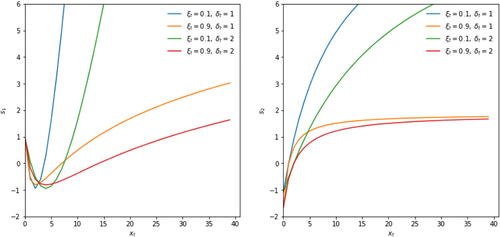
The news impact curves become increasingly concave for lower values of ξ_t. For such parameters, large x_t values are already more likely due to the fat-tailed nature of the GPD itself. As a result, the parameters need to be adjusted less if a large x_t actually materializes. This resembles the well-known robustness properties of score-driven updates in the context of time-varying volatility modeling; see Creal, Koopman, and Lucas (2013) and Harvey (2013). It also distinguishes our current set-up sharply from an approach directly based on quantile functions; see Patton, Ziegel, and Chen (2019) and Catania and Luati (in press), in particular for risk measures such as ES. In Patton, Ziegel, and Chen (2019), ES reacts linearly rather than concavely to the VaR exceedance. This can result in noisy or unstable ES estimates. Figure 1 illustrates that the score-driven approach is less susceptible to such instabilities and can therefore result in more interpretable parameter paths.

We also note that small realizations of x_t imply downward adjustments of both ξ_t and δ_t, up to the point where x_t becomes very small. For very small $x_t>0$, ξ_t is adjusted upward: observations near the center of a fat-tailed distribution signal increased peakedness (=leptokurtosis) and thus higher ξ_t; compare Lucas and Zhang (2016) for a similar effect in the Student’s t setting.

When there is no tail observation, that is $x_t=y_t-{\tau }_t\le 0$, the new observation carries no information about ξ_t and δ_t; see (McNeil, Frey, and Embrechts, 2010, Chapter 7). In such cases we set the score to zero and continue to use (4) to update f_t. Long consecutive stretches of zero scores could potentially lead to mean-reverting paths for f_t, and thus $({\xi }_t,{\delta }_t)$, with only discrete “jumps” when new observations $x_t>0$ arrive following such stretches.² If so, smoothing the scaled score (7) can help to spread out the impact of the new information in x_t. Smoothing the scaled scores can also help when additional conditioning variables z_t are available at every $t=1,\dots ,T$; see (9) and (11) below. Lagged values of the scaled score can be taken into account via an exponentially-weighted moving average specification (8) $$\begin{array}{cc}{f}_{t+1}\hfill & =\omega +A{\tilde{s}}_t+B{f}_t,\mathrm{\hspace{1em}}\mathrm{\hspace{1em}}{\tilde{s}}_t=(1-\lambda )s_t+\lambda {\tilde{s}}_{t-1},\mathrm{\hspace{1em}}\mathrm{\hspace{1em}}\Rightarrow \hfill \\ f_{t+1}\hfill & =(1-\lambda )\omega +(1-\lambda )A{s}_t+(\lambda {\mathrm{I}}_2+B)f_t-\lambda B{f}_{t-1},\hfill \end{array}$$(8) where $\lambda \in [0,1)$ is an additional parameter to be estimated or to be fixed ex-ante; see Web Appendix A.3 for the derivation. This alters the values of $(p,q)=(1,1)$ in (4) to $(p,q)=(2,1)$. While s_t is most often zero, ${\tilde{s}}_t$ is not. Clearly, (4) is a special case of (8) for λ = 0. The smoothing approach in (8) is similar to the approach in Patton (2006), who uses up to 10 lags of the driver (in our case the score) to smooth the dynamics of the time-varying parameter.

The transition equation for f_t can be extended further if additional conditioning variables are available by respecifying (8) as (9) $$f_{t+1}=\omega +A\widetilde{s_t}+B{f}_t+C{z}_t,$$(9) where all explanatory variables are stacked into the column vector z_t, and C is a conformable matrix of impact coefficients that needs to be estimated. We illustrate this in our second application in Section 4.

2.1.3 Time-Varying Thresholds

For the dynamic thresholds τ_t, we use the specification suggested by Patton, Ziegel, and Chen (2019), (10) $${\tau }_{t+1}={\omega }^{\tau }+a^{\tau }·(1\{y_t>{\tau }_t\}-(1-\kappa ))+b^{\tau }{\tau }_t,$$(10) where ${\omega }^{\tau }\equiv (1-b^{\tau })·{\widehat{q}}^{\kappa }$, ${\widehat{q}}^{\kappa }$ is the (observed) unconditional κ-quantile of y_t, $a^{\tau }>0$ and $0<b^{\tau }<1$ are two parameters to be estimated, and $(1-\kappa )$ is a sufficiently small tail probability corresponding to the dynamic quantile τ_t, such as, for example, 10% or 5%. We initialize τ_t at ${\tau }_1={\widehat{q}}^{\kappa }$. The recursive specification (10) is driven by a zero mean innovation process since $\mathbb{E}[1\{y_t>{\tau }_t\left\}\right|{\mathcal{F}}_{t-1},{\theta }^{\tau }]=(1-\kappa )$. The threshold ${\tau }_{t+1}$ responds to quantile exceedances in an intuitive way: the next quantile value ${\tau }_{t+1}$ receives a positive shock of $a^{\tau }\kappa$ if $y_t>{\tau }_t$, that is, if the previous quantile was exceeded, and a negative shock of $-a^{\tau }(1-\kappa )$ otherwise. For $0<b^{\tau }<1$, the empirical unconditional quantile ${\widehat{q}}^{\kappa }$ serves as a long-term attractor for (10). The transition equation for τ_t can also easily be extended to include exogenous variables z_t as in (11) $${\tau }_{t+1}={\omega }^{\tau }+a^{\tau }·(1\{y_t>{\tau }_t\}-(1-\kappa ))+b^{\tau }·{\tau }_t+c^{\tau }\prime ·z_t,$$(11) for a suitable column vector of coefficients $c^{\tau }$.

2.1.4 Interpretation of Time-Varying Parameters

It is important to briefly comment on parameter interpretability. The tail shape parameter ξ_t can always be interpreted as observation y_t’s inverse conditional tail index ${\alpha }_t^{-1}$. By contrast, the estimated tail scale parameter δ_t need not have a straightforward interpretation in terms of y_t’s conditional scale σ_t. For example, assume that y_t has a GPD conditional distribution with time-varying tail shape parameter ${\alpha }_t^{-1}$ and scale σ_t. Web Appendix B.1 demonstrates that the conditional tail probability $\mathbb{P}[Y_t\le y_t+{\tau }_t|Y_t>{\tau }_t,{\mathcal{F}}_{t-1}]$ then also has a GPD shape (exactly, not only approximately). The tail shape parameter is the same as that of the center: ${\xi }_t={\alpha }_t^{-1}$. However, the tail scale parameter δ_t is very different from the scale parameter σ_t that applies to the center, in particular ${\delta }_t={\sigma }_t+{\alpha }_t^{-1}·{\tau }_t$. As a result, δ_t increases with the threshold τ_t, varies positively with the tail shape parameter ξ_t, and, importantly, should not be expected to provide a good estimate of the scale parameter σ_t that applies to the center of the distribution of y_t. A similar result can be derived if y_t were Student’s t-distributed with scale σ_t and degrees of freedom parameter α_t when the tail probability $\mathbb{P}[Y_t\le y_t+{\tau }_t|Y_t>{\tau }_t,{\mathcal{F}}_{t-1}]$ only has an approximate GPD shape; see Web Appendix B.2. We return to this issue in our simulation Section 3, where we consider pseudo-true values for ξ_t and δ_t to benchmark how well the model performs in terms of tracking an unknown data generating process.

2.2 Stationarity and Moments

The score-driven dynamics for ξ_t and δ_t are highly nonlinear. Still, the structure of the model allows us to obtain sufficient conditions for the stationarity and ergodicity (SE) of f_t and x_t, and for the existence of unconditional moments of f_t. To this end, we look at our statistical model in (4)–(8) as a data generating process (DGP).

Given the bivariate structure of our time-varying parameter model, the process ${\left\{f_t\right\}}_{t\in \mathbb{Z}}$ can be viewed as a stochastic recurrence equation (SRE) of the form (12) $$f_{t+1}={\Phi }_t\left(f_t;{\theta }_0\right)=\Phi \left(f_t,x_t;{\theta }_0\right),\mathrm{\hspace{1em}}\mathrm{\hspace{1em}}t\in \mathbb{Z},$$(12) where $\Phi :{\mathbb{R}}^2\times {\mathbb{R}}^{+}\times \Theta \mapsto {\mathbb{R}}^2$ is a Borel measurable function, and ${\theta }_0\in \Theta$ is the true parameter vector contained in the parameter space $\Theta \subset {\mathbb{R}}^6$. We make the following two assumptions.

Assumption 1.

Assume that x_t is drawn from the GPD distribution defined in (2), such that the random variable ${ϵ}_t:={\xi }_t^{-1}\hspace{0.17em}\ln \hspace{0.17em}(1+{\xi }_t x_t/{\delta }_t)$ is an independent and identically distributed noise term with unit exponential distribution, ${ϵ}_t\stackrel{\text{iid}}{\sim }\mathcal{E}xp(1)$.

Assumption 2.

For some integer $r\ge 1$, let (13) $$\mathbb{E}\left[\ln \hspace{0.17em}\underset{f}{\sup }\Vert \prod _{i=1}^r{\dot{\Phi }}_{t-i}\left(f_{t-i};{\theta }_0\right)\Vert \right]<0,$$(13) where $\Vert M\Vert =\sqrt{\mathrm{trace}(M\prime M)}$ is the Frobenius norm of a real-valued matrix $M\in {\mathbb{R}}^{m\times n}$, and where ${\dot{\Phi }}_t(f_t;{\theta }_0):=B+A\frac{\partial {\tilde{s}}_t}{\partial s_t^{\prime }}·\frac{\partial s_t}{\partial f_t^{\prime }}$, such that (14) $${\dot{\Phi }}_t\left(f_t;{\theta }_0\right):=\left(\begin{array}{cc}{b}^{\xi }+a^{\xi }\left(1-\lambda \right)·\frac{\partial s_t^{\xi }}{\partial f_t^{\xi }}& 0\\ a^{\delta }\left(1-\lambda \right)·\frac{\partial s_t^{\delta }}{\partial f_t^{\xi }}& b^{\delta }\end{array}\right),$$(14) with $$\begin{array}{c}\frac{\partial s_t^{\xi }}{\partial f_t^{\xi }}=-{\xi }_t^{-1}{ϵ}_t-{\xi }_t{ϵ}_t\hspace{0.17em}\exp \hspace{0.17em}(-{\xi }_t{ϵ}_t)+(3{\xi }_t^{-1}+2{\xi }_t^{-2})\\ \hspace{1em}\times (1-\hspace{0.17em}\exp \hspace{0.17em}(-{\xi }_t{ϵ}_t))-({\xi }_t+3+{\xi }_t^{-1}){ϵ}_t\hspace{0.17em}\exp \hspace{0.17em}(-{\xi }_t{ϵ}_t)\\ \frac{\partial s_t^{\delta }}{\partial f_t^{\xi }}=\frac{1}{\sqrt{1+2{\xi }_t}}\left(1-\hspace{0.17em}\exp \hspace{0.17em}(-{\xi }_t{ϵ}_t)-{\xi }_t\hspace{0.17em}\exp \hspace{0.17em}(-{\xi }_t{ϵ}_t)\right)\\ \hspace{1em}+\sqrt{1+2{\xi }_t}·(-{\xi }_t^{-1}(1-\hspace{0.17em}\exp \hspace{0.17em}(-{\xi }_t{ϵ}_t))+{ϵ}_t\hspace{0.17em}\exp \hspace{0.17em}(-{\xi }_t{ϵ}_t)\\ \hspace{1em}+{\xi }_t{ϵ}_t\hspace{0.17em}\exp \hspace{0.17em}(-{\xi }_t{ϵ}_t)).\end{array}$$

Assumption A1 considers the model as the data generating process. By inverting the GPD cdf in (2), we obtain that ${ϵ}_t={\xi }_t^{-1}\hspace{0.17em}\ln \hspace{0.17em}(1+{\xi }_t x_t/{\delta }_t)=-\hspace{0.17em}\ln \hspace{0.17em}(1-u_t)\sim \mathcal{E}xp(1)$ for a standard uniformly distributed u_t. Assumption A1 requires that these uniform random variables constitute an iid process.

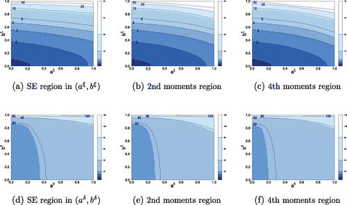
Assumption A2 requires contraction properties of the bivariate stochastic recurrence equation. We note that we use the general form of the r-fold contractions, that is, r iterations of the transition equation of f_t. In univariate models, sharp contraction conditions (that ensure stationarity and ergodicity of the model) can usually be found by assuming that r = 1; see, for example, Blasques et al. (2022). In multivariate systems, however, the contraction condition with r = 1 is often violated, resulting in very small or uninteresting stationarity regions. Working with the more general condition is therefore important. We also show this in Figure 2. The idea behind A2 is that, when working with a multivariate system, one can still ensure the existence of an SE solution if the system becomes contractive eventually, that is, after a sufficiently large number of r iterations. The contraction condition in A2 results in a meaningful (nondegenerate) SE region, because the supremum of ${\dot{\Phi }}_t(f_t;{\theta }_0)$ over f has no degeneracies.

Fig. 2 Stationarity and moments regions.

Top row: the combinations of $a^{\xi }$ and $b^{\xi }$ that satisfy A2 (left panel), and (15) for p = 2 (middle panel) and p = 4 (right panel), for an increasing number of iterations $r\ge 1$. Bottom row: similar, but for combinations of $a^{\delta }$ and $b^{\delta }$ instead. Other deterministic parameters for each panel are fixed at their empirical estimates for S&P500 returns; see Section 4.1.

Using A1 and A2, we can verify the conditions of (Bougerol, 1993, Theorem 3.1). This allows us to show that a unique SE solution exists for the bivariate score-driven process ${\left\{f_t\right\}}_{t\in \mathbb{Z}}$, and for the data ${\left\{x_t\right\}}_{t\in \mathbb{Z}}$ as generated by the DGP in Section 2.1. We summarize this in the following theorem.

Theorem 1.

Consider the model as defined by (2) and (4). Then under A1 and A2, the SRE in (12) admits a unique stationary and ergodic solution ${\left\{{\tilde{f}}_t\right\}}_{t\in \mathbb{Z}}$ such that, for each fixed initial condition $f_0\in {\mathbb{R}}^2$, $$\Vert f_t-{\tilde{f}}_t\Vert \stackrel{e.a.s.}{\to }0\mathrm{\hspace{1em}}\mathrm{\hspace{1em}}\text{as}\mathrm{\hspace{1em}}\mathrm{\hspace{1em}}t\to \infty ,$$where $\stackrel{e.a.s.}{\to }$ denotes exponentially fast and almost sure convergence (Straumann and Mikosch, 2006). In addition, the process ${\left\{x_t\right\}}_{t\in \mathbb{Z}}$ generated by the model evaluated at θ₀ is stationary and ergodic.

Web Appendix C.1 presents the proof of Theorem 1. Next to the SE properties of the f_t process, we can also establish the existence of unconditional moments. This can be useful for proving the existence of moments of the log-likelihood function and its derivatives. We note that the contraction condition stated in A2 by its own is insufficient to ensure bounded unconditional moments of f_t in the DGP. Requiring the existence of moments typically makes the admissible parameter space smaller. We also note that the existence of unconditional moments of f_t does not imply the same (un)conditional moments for x_t. For instance, even if f_t has a finite 4th order moment, x_t may not if ξ_t can reach levels higher than 1/4. We have the following result.

Theorem 2.

Consider the model as defined by (2) and (4), and let A1 and A2 be true. If in addition (15) $$\mathbb{E}\left[\underset{f}{\sup }{\Vert \prod _{i=1}^r{\dot{\Phi }}_{t-i}\left(f_{t-i};{\theta }_0\right)\Vert }^p\right]<1,$$(15) for some $p\ge 1$, then the unique stationary and ergodic solution ${\left\{{\tilde{f}}_t\right\}}_{t\in \mathbb{Z}}$ to the SRE in (12) satisfies $\mathbb{E}[⏧{\tilde{f}}_t{⏧}^p]<\infty$.

Web Appendix C.2 provides the proof of Theorem 2. Again, Theorem 2 makes use of r-fold contraction conditions rather than the standard r = 1 case.

To give some insight into the size of the SE and moments regions, we compute them numerically in Figure 2. We let two (out of the six) parameters in Θ vary at a time. Computing the regions is far from trivial. It requires numerically solving a maximization problem embedded inside an integration problem. As a result, the maximization problem has to be solved for every value of the integration variable. Details are provided in Web Appendix D.

Figure 2 clearly illustrates the importance of multiple unfoldings of the SRE. If only r = 1 iteration is used, the SE and finite-moments regions are typically small, or even empty; see for instance the small darkest blue region in panel 2(a) for r = 1, or the fact that panel 2(d) only shows contracting behavior for $r\ge 17$ iterations given the empirical estimates. For r = 1, empirical estimates typically lie outside the SE region. However, by iterating the SRE forward, the SE and finite-moments regions grow considerably to the extent that they also encompass the empirical estimates. For instance, the model may not be SE when evaluated at the empirical estimates for r = 1. For r = 20, 40, or even larger, however, the model’s SE region at the empirical estimates increases such that even fourth order moments of f_t exist. Given the S&P500 data (on which Figure 2 is based) are at a daily frequency, we conclude that a time-varying parameter model may not have guaranteed contraction properties at the daily frequency, but may still have such contraction properties at a monthly (r = 22) or lower frequency. The numerical results in the figure stress that analytical conditions for SE, as often encountered in the literature for r = 1, may be quite uninteresting if not accompanied by a numerical check for the size of the resulting parameter space.

2.3 Parameter Estimation

Observation-driven time series models such as (1)–(11) have the appealing feature that the log-likelihood is known in closed form. For a given set of time series observations $x_t=1\{y_t>{\tau }_t\}·(y_t-{\tau }_t)$ for $t=1,\dots ,T$, the vector of unknown parameters θ can then be estimated by maximizing the log-likelihood function of the GPD with respect to θ. The average log-likelihood function is given by (16) $$\begin{array}{c}\mathcal{L}\left(\theta |{\mathcal{F}}_T\right)=\frac{1}{T^{*}}\sum _{t=1}^{T}1\{x_t>0\}·\hspace{0.17em}\ln \hspace{0.17em}p(x_t;{\delta }_t,{\xi }_t)\\ =\frac{1}{T^{*}}\sum _{t=1}^{T}1\{x_t>0\}\\ \hspace{1em}·\left[-\hspace{0.17em}\ln \hspace{0.17em}({\delta }_t)-\left(1+\frac{1}{{\xi }_t}\right)\hspace{0.17em}\ln \hspace{0.17em}\left(1+{\xi }_t\frac{x_t}{{\delta }_t}\right)\right],\end{array}$$(16) where $T^{*}={\sum }_{t=1}^{T}1\{x_t>0\}$ is the number of POT values in the sample. Maximization of (16) can be carried out using a conveniently chosen quasi-Newton optimization method.

To establish consistency and asymptotic normality of the maximum likelihood estimator (MLE), we define the MLE θ̂ as (17) $$\widehat{\theta }:=\underset{\theta \in \Theta }{\text{argmax}}\mathcal{L}\left(\theta |{\mathcal{F}}_T\right).$$(17)

We establish these asymptotic properties by showing that the conditions for Lemma 1 in Jensen and Rahbek (2004) are satisfied. The main point to note is that the first three derivatives of the $\hspace{0.17em}\log \hspace{0.17em}$-likelihood function (and of f_t) with respect to θ are stationary and ergodic stochastic recurrence equations that satisfy specific moment conditions. We make the following additional assumption on the parameter space Θ.

Assumption 3.

The parameter vector $\theta \in \Theta$ for a compact parameter space $\Theta \subset {\mathbb{R}}^6$, and the true parameter vector ${\theta }_0\in \text{int}(\Theta )$. Additionally, for each $\theta \in \Theta$, the starting value $f_0(\theta )=(\hspace{0.17em}\ln \hspace{0.17em}({\xi }_0),\hspace{0.17em}\ln \hspace{0.17em}({\delta }_0))\prime \in {\mathbb{R}}^2$ is fixed to the true value.

Finally, we impose conditions on the score vector ${\nabla }_t$, as defined in (5), and its derivatives up to third-order. Let ${\nabla }_t(\theta ),{\nabla }_t^2(\theta )$ and ${\nabla }_t^3(\theta )$ denote the score vector and first two derivatives with respect to $f_t^{\xi }(\theta )$ and $f_t^{\delta }(\theta )$, evaluated at some $\theta \in V({\theta }_0)$, where $V({\theta }_0)$ denotes a small neighborhood of the true parameter vector θ₀. By imposing the conditions in Assumption 4, we can rule out explosive behavior of the first three derivatives of the $\hspace{0.17em}\log \hspace{0.17em}$-likelihood function with respect to θ. Similar boundedness assumptions have been used in for instance Hetland, Pedersen, and Rahbek (in press) or Hafner and Wang (in press). Effectively, this further reduces the size of the parameter space (see also Blasques et al., 2022). Web Appendix E.1 provides the explicit analytic expressions for each of these derivatives.

Assumption 4.

The score vector ${\nabla }_t(\theta )$, and its derivatives ${\nabla }_t^2(\theta )$, and ${\nabla }_t^3(\theta )$ are p-dominated uniformly in $V({\theta }_0)$ and t by dominating functions $D_{1,t},D_{2,t}$, and $D_{3,t}$, respectively, such that $$\begin{array}{c}\underset{\theta \in V({\theta }_0)}{\sup }\Vert {\nabla }_t(\theta )\Vert \le D_{1,t},\mathrm{\hspace{1em}}\mathrm{\hspace{1em}}\underset{\theta \in V({\theta }_0)}{\sup }\Vert {\nabla }_t^2(\theta )\Vert \le D_{2,t},\mathrm{\hspace{1em}}\mathrm{\hspace{1em}}\text{and}\\ \underset{\theta \in V({\theta }_0)}{\sup }\Vert {\nabla }_t^3(\theta )\Vert \le D_{3,t},\end{array}$$where $D_{1,t},D_{2,t}$, and $D_{3,t}$ are p-integrable uniformly in t for p > 0, that is ${\Vert D_{1,t}\Vert }^p\le {\Delta }_1<\infty$, ${\Vert D_{2,t}\Vert }^p\le {\Delta }_2<\infty$, and ${\Vert D_{3,t}\Vert }^p\le {\Delta }_3<\infty$.

The following theorem establishes the asymptotic properties of our MLE.

Theorem 3.

Consider the model as defined by (2) and (4). Let Assumptions 1–3 hold true. Then $\widehat{\theta }\stackrel{P}{\to }{\theta }_0$ as $T^{*}\to \infty$.

If, in addition, Assumption 4 holds true, as well as the contraction condition (15) in Theorem 2 for p = 4, then $\sqrt{T^{*}}(\widehat{\theta }-{\theta }_0)\Rightarrow \mathrm{N}(0,{\Omega }_I^{-1})$ as $T^{*}\to \infty$, where Ω_I denotes the Fisher information matrix evaluated at the true parameter vector θ₀.

The proof of Theorem 3, together with detailed derivations of the derivatives up to the third-order of the $\hspace{0.17em}\log \hspace{0.17em}$-likelihood function $\mathcal{L}(\theta |{\mathcal{F}}_T)$, and of the (bivariate) score-driven process ${\{f_t(\theta )\}}_{t\in \mathbb{Z}}$, for each $\theta \in \Theta$ can be found in Web Appendix E.2.

All our results are conditional on the time-varying thresholds τ_t. The parameters $a^{\tau }$ and $b^{\tau }$ for τ_t in (10) cannot be estimated using (16). Another objective function is needed in this case. We suggest using the average quantile regression check function of (Koenker, 2005, chap. 3). The optimization problem can be formulated as (18) $$\begin{array}{c}{\min }_{\{a^{\tau },\mathrm{ }{b}^{\tau }\}}\frac{1}{T}\sum _{t=1}^T{\rho }_{\kappa }\left(y_t-{\tau }_t\right)\\ \iff {\min }_{\{a^{\tau },\mathrm{ }{b}^{\tau }\}}\frac{1}{T}\sum _{t=1}^T(y_t-{\tau }_t)\left(\kappa -1\{y_t<{\tau }_t\}\right)\\ \iff {\max }_{\{a^{\tau },\mathrm{ }{b}^{\tau }\}}\frac{1}{T}\sum _{t=1}^T(y_t-{\tau }_t)\left((1-\kappa )-1\{y_t>{\tau }_t\}\right),\end{array}$$(18) where ${\rho }_{\kappa }(u_t)=u_t(\kappa -1\{u_t<0\})$, and τ_t evolves as in (10). See also Engle and Manganelli (2004) and Catania and Luati (in press) for the use of this objective function in a different dynamic context. In practice, we estimate all thresholds τ_t via (18) before maximizing (16).

2.4 Confidence Bands for Tail Shape and Tail Scale

Given the maximum likelihood estimate $\widehat{\theta }$, confidence (or standard error) bands around ${\widehat{f}}_t=f_t(\widehat{\theta })$ allow us to visualize the impact of estimation uncertainty. Quantifying the uncertainty of the estimated parameter paths is important, as classical EVT estimators of time-invariant tail shape parameters can have sizeable standard errors; see for example, Hill (1975) and Huisman et al. (2001). Web Appendix F explains how simulation-based and in-sample analytic confidence bands around ${\widehat{f}}_t$ can be obtained. These bands are conditional on the estimated time-varying thresholds ${\widehat{\tau }}_t$, and do not incorporate the associated estimation uncertainty of the thresholds.

2.5 Market Risk Measures

Market risk measurement is a major application of EVT methods in practice; see for example, McNeil, Frey, and Embrechts (2010). The GPD approximation (1)–(2) yields useful closed-form estimators of the VaR and ES for high upper quantiles $\gamma >G({\tau }_t|{\mathcal{F}}_{t-1})$; see McNeil and Frey (2000) and Rocco (2014). We can estimate the $1-\gamma$ tail probability of y_t based on the GPD cdf for x_t, obtaining ${\text{VaR}}^{\gamma }(y_t|{\mathcal{F}}_{t-1},\theta )={\tau }_t+{\delta }_t{\xi }_t^{-1}\left[{\left(\frac{1-\gamma }{t^{*}/t}\right)}^{-{\xi }_t}-1\right],$ where $t^{*}$ is the number of observations with $x_t>0$ up to time t, that is, the number of y_s for $s=1,\dots ,t$ for $y_s>{\tau }_s$.

The conditional ES is the average conditional VaR in the tail across all quantiles γ (see McNeil, Frey, and Embrechts, 2010, chap. 2), provided ${\xi }_t<1$. The closed-form expression is ${\text{ES}}^{\gamma }(y_t|{\mathcal{F}}_{t-1},\theta )=\frac{{\text{VaR}}^{\gamma }(y_t|{\mathcal{F}}_{t-1},\theta )}{1-{\xi }_t}+\frac{{\delta }_t-{\xi }_t{\tau }_t}{1-{\xi }_t},$ see Web Appendix G for a derivation of the equations. Maximum likelihood estimators of the conditional VaR and conditional ES can be obtained by inserting filtered estimates of ξ_t and δ_t into the VaR and ES equations, respectively.

3 Simulation Study

3.1 Simulation Design

This section investigates the ability of our dynamic EVT model to simultaneously recover (i) the time variation in tail shape and tail scale parameters ξ_t and δ_t, (ii) EVT-based market risk measures VaR ${}^{\gamma }(y_t;{\tau }_t,{\xi }_t,{\delta }_t)$ and ES ${}^{\gamma }(y_t;{\tau }_t,{\xi }_t,{\delta }_t)$ at high confidence levels such as $\gamma =99\%$, and (iii) parameter estimates and their standard errors for all deterministic parameters collected in θ. We do so using two sets of data generating processes (DGPs). The first set of DGPs is discussed in the main text, while the second set of DGPs is discussed in Web Appendix H. In our experiments, we track the performance of our score-driven modeling approach when putting it into a variety of challenging settings, such as when the conditional density is only approximately correct, the time-varying parameter process is misspecified or features (near)-unit roots, and/or when both tail parameters follow similar paths. We also investigate whether the market risk estimates that follow from the model are reliable.

In our first set of DGPs, we consider D = 2 different densities (GPD and Student’s t), P = 4 different parameter paths for tail shape and scale, and H = 3 different ways to obtain the appropriate thresholds τ_t. This yields $2\times 4\times 3=24$ simulation experiments. In each experiment, we draw S = 100 univariate simulation samples of length $T=25,000$. We focus on the upper $1-\kappa =5$% tail. As a result, approximately $25,000·0.05=1250$ observations are available in each simulation to compute informative POTs $x_t>0$.

We first simulate y_t from a GPD $({\alpha }_t^{-1},{\sigma }_t)$ distribution with time-varying tail shape ${\alpha }_t^{-1}$ and scale σ_t. In a second set-up, we consider a Student’s t distribution with time-varying scale σ_t and degrees of freedom α_t. In the GPD case, our score-driven model uses the exact conditional density for x_t, while in the t case the GPD conditional density for x_t is only approximately correct (given finite thresholds τ_t in any given sample); see Web Appendix B.

We consider four different paths for the tail shape ${\alpha }_t^{-1}$ and scale σ_t parameters. For both the GPD and Student’s t densities we consider

1. Constant: ${\alpha }_t^{-1}=0.5,{\sigma }_t=1$;

2. Sine and constant: ${\alpha }_t^{-1}=0.5+0.3\hspace{0.17em}\sin \hspace{0.17em}(4\pi t/T),{\sigma }_t=1$;

3. Slow sine and frequent sine: ${\alpha }_t^{-1}=0.5+0.3\hspace{0.17em}\sin \hspace{0.17em}(4\pi t/T),{\sigma }_t=1+0.5\hspace{0.17em}\sin \hspace{0.17em}(16\pi t/T)$;

4. Synchronized sines: ${\alpha }_t^{-1}=0.5+0.3\hspace{0.17em}\sin \hspace{0.17em}(4\pi t/T),{\sigma }_t=1+0.5\hspace{0.17em}\sin \hspace{0.17em}(4\pi t/T)$.

Consequently, paths (1) considers the special case of time-invariant tail shape and scale parameters. Naturally, we would want our dynamic framework to cover constant parameters as a special case. Paths (2) allows the tail shape to vary considerably between 0.2 and 0.8, while keeping the scale (volatility) of the data constant. Paths (3) stipulates that both parameters vary over time. Finally, paths (4) considers the case of synchronized variation in both parameters.

Next, we consider three ways to construct the thresholds τ_t. First, we use the true time-varying 95%–quantile based on our knowledge of the true density and of α_t and σ_t. This constitutes an infeasible best benchmark. Second, we construct τ_t as the 95%–quantile of the expanding window of data up to time t, that is ${\tau }_t=Q_{1:t}^{0.95}(\{y_1,\dots ,y_t\})$. Finally, we use the recursive specification (10), initialized at the full-sample quantile ${\tau }_1=Q_{1:T}^{0.95}$.

Our main evaluation metric for evaluating model performance is the root mean squared error $\text{RMSE}=\frac{1}{S}{\sum }_{s=1}^S\sqrt{\frac{1}{T}{\sum }_{t=1}^T{({\widehat{\xi }}_t^s-{\overline{\xi }}_t^s)}^2}$, where ${\widehat{\xi }}_t^s$ is the estimated tail shape parameter in simulation s, ${\overline{\xi }}_t^s$ is the corresponding (pseudo-)true tail shape, $s=1,\dots ,S$ denotes the simulation run, and $t=1,\dots ,T$ is the number of observations in each draw. The RMSE for the tail scale parameter δ_t is obtained analogously. The pseudo-true values ${\overline{\xi }}_t^s$ and ${\overline{\delta }}_t^s$ are obtained by numerically minimizing the Kullback-Leibler divergence between the GPD and the data generating process beyond the true time-varying 95% quantile τ_t. As the true conditional density is known at all times in a simulation setting, these pseudo-true benchmarks are easily computed numerically for each s and t. Particularly the GPD tail scale parameter ${\overline{\delta }}_t$ may have very different dynamics from σ_t, as it combines dynamics in α_t and σ_t via the EVT limiting expression in (1); see also Section 2.1.4.

3.2 Simulation Results

For the first set of DGPs, we are particularly interested in two issues: first, what is the effect of increasing misspecification by moving from a GPD to a Student’s t density in the data generating process of y_t, and second, how accurately can we recover high-confidence market risk measures when the conditional GPD density is only approximately correct.

Table 1 presents the corresponding results. It reports RMSE statistics for tail shape ξ̂ and tail scale ${\widehat{\delta }}_t$. Figure 3 provides a representative example of the simulation outcomes where we compare median estimated parameter paths for ${\widehat{\xi }}_t,{\widehat{\delta }}_t,{\widehat{\text{VaR}}}^{0.99}$, and ${\widehat{\text{ES}}}^{0.99}$ to their (pseudo)-true values. Full results are found in Web Appendix H.1. The true parameters in Figure 3 follow Path 3 from Section 3.1, and time-varying thresholds are estimated based on the recursive specification (10) and objective function (18).

Fig. 3 Simulation results: an example.

Time series data is here generated as $y_t\sim$t$(0,{\sigma }_t,{\alpha }_t)$, where ${\alpha }_t^{-1}=0.5+0.3\hspace{0.17em}\sin \hspace{0.17em}(4\pi t/T)$ and ${\sigma }_t=1+0.5\hspace{0.17em}\sin \hspace{0.17em}(16\pi t/T)$. This is Path 3 in Section 3.1. Pseudo-true parameter values are reported in solid red. The four panels report estimates of ξt, δt, VaRt, and ESt, respectively. Median filtered values are plotted in solid black. The first two panels also indicate the lower 5% and upper 95% quantiles of the estimates (black dots). The time-varying threshold ${\widehat{\tau }}_t$ is estimated based on the recursive specification (10) in conjunction with the objective function (18).

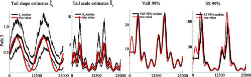
Table 1 RMSE outcomes for DGP1.

Model	GPD(τt)	GPD(${\widehat{\tau }}_t$)	GPD(${\widehat{\tau }}_t^{*}$)	t(τt)	t(${\widehat{\tau }}_t$)	t(${\widehat{\tau }}_t^{*}$)
	(infeasible)			(infeasible)
	RMSE ${\widehat{\xi }}_t$
(1)	0.000	0.000	0.000	0.000	0.000	0.000
	(0.000)	(0.000)	(0.000)	(0.000)	(0.000)	(0.000)
(2)	0.171	0.177	0.178	0.182	0.188	0.189
	(0.002)	(0.002)	(0.002)	(0.002)	(0.002)	(0.002)
(3)	0.182	0.188	0.189	0.190	0.197	0.197
	(0.002)	(0.002)	(0.002)	(0.002)	(0.002)	(0.002)
(4)	0.177	0.186	0.183	0.188	0.195	0.192
	(0.002)	(0.002)	(0.002)	(0.002)	(0.002)	(0.002)
	RMSE ${\widehat{\delta }}_t$
(1)	0.005	0.014	0.068	0.005	0.010	0.034
	(0.003)	(0.006)	(0.013)	(0.002)	(0.004)	(0.006)
(2)	1.646	1.774	1.753	0.580	0.589	0.588
	(0.034)	(0.040)	(0.036)	(0.013)	(0.012)	(0.013)
(3)	2.421	2.913	2.813	0.836	0.960	0.924
	(0.054)	(0.054)	(0.049)	(0.015)	(0.020)	(0.017)
(4)	2.608	2.904	2.844	0.925	0.970	0.964
	(0.057)	(0.059)	(0.059)	(0.020)	(0.020)	(0.022)

NOTE: Root mean squared error (RMSE) statistics for two different distributions (GPD and t, in columns) and for four different parameter paths for tail shape ξ_t and tail scale δ_t (paths (1)–(4), in rows). Thresholds τ_t, ${\widehat{\tau }}_t$, and ${\widehat{\tau }}_t^{*}$ denote, respectively, (i) the infeasible true time-varying threshold, (ii) the empirical quantile associated with an expanding window of observations $y_1,\dots ,y_t$, and (iii) the estimated conditional quantile using (18) and a suitably calibrated $a^{\tau }=0.25$ to speed up the computations. We consider 100 simulations for each DGP, and a time series of 25,000 observations in each simulation. Model performance is measured by the RMSE from the true ${\overline{\xi }}_t$ and ${\overline{\delta }}_t$ in each draw.

We focus on three main findings. First, all models seem to work well in recovering the true underlying ξ_t and δ_t dynamics. The median estimates in Figure 3 tend to be close to their (pseudo)-true values. The full results in in Web Appendix H.1 confirm this. Even the highly nonlinear patters of δ_t are recovered well. The model also captures the peaks of ξ_t, which correspond to the episodes with the fattest tails. The model needs some time to recognize that the extreme tail has become more benign, that is, that ξ_t has gone down. The good fit is corroborated by Table 1. We also note that both estimation methods for τ_t only loose about 10% RMSE for ξ_t and δ_t compared to the use of the true (infeasible) τ_t.

Second, when comparing the results for ξ_t and δ_t based on the recursive estimate ${\widehat{\tau }}_t$ and the dynamic estimate ${\tau }_t^{*}$ of Patton, Ziegel, and Chen (2019), Table 1 shows differences are mostly small and insignificant. If there is no time-variation (Path 1), the estimates of ${\widehat{\delta }}_t$ based on a recursive ${\widehat{\tau }}_t$ fare slightly better (as expected). The converse is true for if the true parameters vary over time (Paths 2–4).

Third, Figure 3 shows that EVT-based market risk measures such as high-confidence level ($\gamma =0.99$) VaRs and ESs tend to be estimated sufficiently accurately with our dynamic EVT approach. Again, this is confirmed by the full results in Web Appendix H.1. Both the low and high frequency dynamics of VaR and ES are captured well. There only appears some under-estimation of the ES at its highest peak, where tails are extremely fat. Overall, we conclude that the model captures the dynamics of the tails accurately, even in cases where the model does not coincide with the true, unobserved data generating process and the model is thus misspecified.

We conclude this section by briefly summarizing the main simulation results from our second set of DGPs in Web Appendix H.2. Empirical estimates of the autoregressive parameters $b^{\xi }$ and $b^{\delta }$ can be close to one; see Section 4. For this reason, we investigate the effect of (near-)unit root type dynamics and of additional covariates on the parameter estimates and their standard errors. We find that models with (near-)unit root type dynamics continue to work reliably. The estimated $\widehat{\delta },{\widehat{\xi }}_t$, and ${\widehat{\delta }}_t$ continue to be closely aligned to their true values. The usual asymptotic standard error estimates based on the inverse Hessian or sandwich estimates, however, are not always reliable then. In our set-up, these common estimates of the standard errors are typically too large, providing too conservative inference. A bootstrap procedure tailored to integrated processes could then be used to avoid this issue.³

4 Empirical Illustrations

4.1 Equity Log-Returns

To illustrate our approach, we obtain end-of-day prices for the S&P500 index and for IBM stock as two easily and publicly available series from the CRSP database.⁴ The S&P500 data range from July 3, 1962 to December 31, 2020, yielding 14,726 daily observations. The IBM stock data range from January 2, 1926 to December 31, 2020, yielding 25,028 daily observations. To model the adverse left tail of equity log-returns we consider negative log-returns $y_t=-100\times (\hspace{0.17em}\ln \hspace{0.17em}{p}_t-\hspace{0.17em}\ln \hspace{0.17em}{p}_{t-1})$, with p_t the price level, before applying our methodology.

4.1.1 Deterministic Parameter Estimates

We rely on the time-variation in the thresholds τ_t to accommodate time-variation in any parameters describing the center of the distribution. The thresholds evolve over time according to (10), at $(1-\kappa )=10\%$, and are initialized at ${\tau }_1={\widehat{q}}^{0.9}$, the 90% empirical quantile of y_t. The factor process $f_t=(\hspace{0.17em}\ln \hspace{0.17em}{\xi }_t,\hspace{0.17em}\ln \hspace{0.17em}{\delta }_t)\prime$ is initialized at $f_1={({\mathrm{I}}_2-B)}^{-1}\omega$.

The first two columns in Table 2 present our estimates of the deterministic parameters of model (1)–(10). The estimates of $a^{\tau }>0$ and $b^{\tau }<1$ suggest that the thresholds are time-varying and mean-reverting. Parameters $a^{\xi }$ and $a^{\delta }$ are statistically significant at any reasonable significance level, for both S&P500 and IBM. These parameters can be interpreted as the average size of the scores driving $\hspace{0.17em}\ln \hspace{0.17em}{\xi }_t$ and $\hspace{0.17em}\ln \hspace{0.17em}{\delta }_t$, respectively; see the statements above (6). Parameters $b^{\xi }$ and $b^{\delta }$ are estimated to be close to one for both series, implying that shocks to each time-varying parameter die out only slowly. A numerical check reveals that the deterministic parameters $a^{\xi }$ and $b^{\xi }$ lie within the SE region implied by the sufficient conditions of Theorems 1 and 2. A diagnostic check in Web Appendix J suggests that the bivariate filter (4) is also invertible at these estimates.

Table 2 Parameter estimates.

	First illustration		Second illustration
	S&P500	IBM	IT 5y yield		PT 5y yield
$a^{\xi }$	0.025	0.018	0.018	0.023	0.028	0.028
	(0.01)	(0.00)	(0.003)	(0.002)	(0.003)	(0.004)
	[0.00]	[0.00]	[0.000]	[0.000]	[0.000]	[0.000]
$a^{\delta }$	0.112	0.088	0.079	0.076	0.092	0.089
	(0.01)	(0.01)	(0.003)	(0.003)	(0.004)	(0.004)
	[0.00]	[0.00]	[0.000]	[0.000]	[0.000]	[0.000]
$b^{\xi }$	0.9993	0.9997	0.9997^a	0.9997^a	0.9997^a	0.9997^a
	(0.00)	(0.00)
	[0.00]	[0.00]
$b^{\delta }$	0.995	0.994	0.9997^a	0.9997^a	0.9997^a	0.9997^a
	(0.001)	(0.001)
	[0.00]	[0.00]
$c^{\xi }$				–7.696		–47.855
				(2.225)		(22.555)
				[0.001]		[0.034]
$c^{\delta }$				0.144		–10.782
				(0.737)		(4.323)
				[0.845]		[0.013]
λ	0	0	0.911	0.911	0.911	0.911
$a^{\tau }$	0.241	0.260	0.221	0.221	0.773	0.773
$b^{\tau }$	0.989	0.990	0.999	0.999	0.998	0.998
$c^{\tau }$			0.017	0.017	–0.141	–0.141
T	14,726	25,028	24,416	24,416	24,576	24,576
$T^{*}$	1495	2532	2448	2448	2490	2490
loglik	–22,028.4	–62,727.4	–80,535.8	–80,513.9	–196,068.0	–196,031.0
AIC	44,068.7	125,466.9	161,079.7	161,039.8	392,143.9	392,074.0
BIC	44,114.3	125,515.7	161,112.1	161,088.4	392,176.3	392,122.7

NOTE: Parameter estimates for the dynamic tail shape model. The second and third columns refer to the first application (equity log-returns of the S&P500 index and IBM stock). The estimation samples range from July 3, 1962 to December 31, 2020 for the S&P500 index, and from January 2, 1926 to December 31, 2020 for IBM stock. The remaining columns refer to the second application (changes in sovereign yields). Columns labeled IT 5y and PT 5y refer to yield changes for Italy and Portuguese five-year benchmark bonds sampled at the 15-min frequency. The estimation samples range from January 4, 2010, 9 a.m., to December 31, 2012, 5 p.m. For the second application, $b^{\xi }$ and $b^{\delta }$ are estimated indistinguishably different from, but still slightly below one. To be in line with theory, we fix the coefficients slightly below 1 at ${0.9997}^a$ for a = 1/32, such that at a daily (8 hr = 32 quarters) the coefficient is comparable to the highest IBM coefficient, $b^{\xi }$. Standard error estimates are in round brackets, p-values are in square brackets. Standard errors and p-values are based on a sandwich covariance matrix estimator for the first application, and on a bootstrap procedure for the second application.

4.1.2 Tail Parameter Estimates

Figure 4 presents the raw log-returns (top panels) along with filtered estimates of ξ_t and δ_t (middle and bottom panels). The filtered tail shape varies between approximately 0.05 and 0.25 for the S&P 500 index, and between approximately 0.05 and 0.35 for IBM. The filtered tail scales vary roughly between 0.2 and 2.0 for the S&P 500 and IBM. The confidence bands around each filtered parameter suggest that both are reasonably precisely estimated, and that the tail shape parameter is often far from zero. The reported confidence bands are conditional on the estimated thresholds ${\widehat{\tau }}_t$.

Fig. 4 Filtered tail parameters for S&P500 (left) and IBM (right) log-returns.

Top panels: daily log-returns for the S&P500 index (left) and IBM common stock (right). Middle and bottom panels: filtered tail shape (ξt, middle) and tail scale (δt, bottom) parameters. The thresholds τt are reported at a 90% confidence level; Value-at-Risk (VaR) and Expected Shortfall (ES) are plotted at an extreme 99% confidence level (top panels). The thresholds τt, VaR, and ES are mirrored at the horizontal axis to correspond to log-returns (instead of percentage losses). The estimation samples range from July 3, 1962 to December 31, 2020 for the S&P500 index, and from January 2, 1926 to December 31, 2020 for the IBM stock. The reported samples range from July 3, 1962 to December 31, 2020.

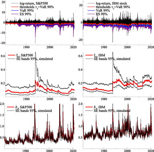
The filtered estimates of ξ_t and δ_t suggest that one-off, extremely negative returns affect the filtered tail shape more than the filtered tail scale. Longer-lasting crises, by contrast, appear to affect the tail scale more than the tail shape. For example, the stock market crash on October 19, 1987, also known as “Black Monday,” considerably increases ${\widehat{\xi }}_t$ but not ${\widehat{\delta }}_t$. Similarly, the 2010 “flash-crash” on May 6, 2010 increases ${\widehat{\xi }}_t$ more than ${\widehat{\delta }}_t$. By contrast, the global financial crisis between 2008 and 2009, and the Covid-19 pandemic recession in early 2020, both temporarily increase ${\widehat{\delta }}_t$ while leaving ${\widehat{\xi }}_t$ less affected.

Figure 4 also plots estimates of VaR_t and ES_t at a 99% confidence level. We checked that indeed 1.0% of the log-returns lie beyond ${\widehat{\text{VaR}}}_t$ in the case of the S&P 500 index (0.9% for IBM stock). The average value of $-y_t$ conditional on it exceeding its VaR is –3.54% for the S&P 500, and –4.85% for IBM. These values are approximately in line with the time series average of ${\widehat{\text{ES}}}_t$ at –3.12% for the S&P 500, and –4.59% for IBM, respectively.

4.2 Changes in Sovereign Yields

In our second application we illustrate the inclusion of explanatory variables in the dynamics of ξ_t and δ_t as in (9). To do so, we study whether there was any tail risk impact of central bank asset purchases on changes in Italian (IT) and Portuguese (PT) five-year bond yields between 2010 and 2012. Both Italy and Portugal were in the “epicenter” of the existential euro area sovereign debt crisis at that time; see for example, Eser and Schwaab (2016), and Ghysels et al. (2017). Italy is an example for a large euro area country that was affected by the crisis relatively late (in mid-2011), and that benefited from Eurosystem bond purchases only during a relatively short period of time, between August 2011 and March 2012. Portugal, by contrast, is an example for a smaller euro area country that was affected relatively early (already in 2010), and that benefited from Eurosystem bond purchases more uniformly over time, between May 2010 and March 2012.

Eurosystem bond purchases undertaken during the sovereign debt crisis predominantly targeted the 1- to 10-year maturity bracket, with the 5-year maturity approximately in the middle of that spectrum; see for example Eser and Schwaab (2016). We consider the impact on five-year sovereign benchmark bond yields for this reason.

The bond yields y_t are sampled at the 15-min frequency, between 9 a.m. and 5 p.m., and are obtained from Bloomberg. We do not consider overnight changes in yield, such that the first 15-min interval covers 9 a.m. to 9:15 a.m. Our sample ranges from January 04, 2010 to December 31, 2012. This yields 32 intra-daily observations per trading day, with $T\approx 3\times 260\times 32\approx 25,000$ observations per country.

Finally, we construct time series data z_t of country-specific bond purchases at the high (15-min) frequency. Observations z_t contain all sovereign bond purchases at par (nominal) value between t – 1 and t for the respective country, not only purchases of the five-year benchmark bond. Disaggregated data on Eurosystem SMP purchases sampled at a high-frequency are still confidential at the time of writing. At the end of our sample, the Eurosystem held €99.0 bn in Italian sovereign bonds and €21.6 bn in Portuguese bonds; see the ECB Annual Report 2013. We including these as an additional conditioning variable in (9) to see whether they mitigated extreme tail behavior or not.

4.2.1 Deterministic Parameter Estimates

We continue to rely on the time-variation in the thresholds τ_t to control for time-variation in any parameters describing the center of the distribution. The thresholds now evolve according to (11), also taking account of the SMP purchases z_t. We choose $(1-\kappa )=10\%$, and initialize ${\tau }_1={\widehat{q}}^{0.9}$, the 90% empirical quantile of y_t.

Analyzing changes in the tail shape and tail scale parameters for high-frequency data is challenging given the high persistence of parameters at such frequencies. We therefore introduce two simplifications. First, we fix the smoothing parameter λ at ${0.05}^{1/32}\approx 0.911$, such that 95% of the smoothing materializes within one day (i.e., 32 15-min intervals). As there are only log-likelihood contribution for the GPD for $x_t=z_t-{\tau }_t>0$, it is hard to identify λ empirically. Second, to keep the model in line with the theory from Section 2.2, we fix $b^{\xi }$ and $b^{\delta }$ to a value close to the unit boundary, as otherwise they are estimated indistinguishably different from 1. We choose ${(b^{\xi })}^{32}={(b^{\delta })}^{32}=0.9997$, which implies a similar persistence level as (IBM) equity returns at a daily (= 8h = 32 quarters) frequency. Fixing λ, $b^{\xi }$, or $b^{\delta }$ at other reasonable values has little effect on the empirical findings.

Columns three to six of Table 2 present our estimates of the deterministic parameters for the model (1)–(11). Columns three and five refer to a baseline model without central bank purchases. Table 2 reports bootstrapped standard errors for the deterministic parameters using the procedure outlined in Web Appendix K.

The estimates of $a^{\tau }>0$ and $b^{\tau }<1$ suggest that the thresholds are time-varying and mean-reverting. Parameter $c^{\tau }$ is estimated to be negative for Portuguese bonds, and close to zero for Italian bonds. Parameters $a^{\xi }$ and $a^{\delta }$ suggest pronounced and statistically significant time series variation in both the tail shape ξ_t and tail scale δ_t parameters, both of which are captured by our time-varying parameter model. The impact parameters $c^{\xi }$ and $c^{\delta }$ of bond purchases on tail shape and scale are estimated to be negative in both cases. The log-likelihood increases by 21.9 points for IT, and 37.0 points for PT. A comparison of model selection criteria (AIC, BIC) further supports the inclusion of central bank asset purchases as a useful covariate to explain each time series’ extreme tail dynamics.

4.2.2 Tail Parameter Estimates and VaR Impact

Figure 5 plots the corresponding filtered estimates for time-varying tail shape ξ_t and tail scale δ_t. Time series variation is present and pronounced in both parameters. The filtered tail shape varies between approximately 0.1 and 0.4 for Italian yields, and between 0.05 and 0.6 for Portuguese yields. The filtered tail scale varies between approximately 1 and 10.0 for Italian yields, and between approximately 1 and 40 for Portuguese yields. The standard error bands around each time-varying parameter suggest that both parameters are estimated reasonably precisely, and that the tail shape is often far from the Gumbel case of ${\xi }_t=0$.

Fig. 5 The tail shape and tail scale estimates.

Top row: Five-year sovereign benchmark bond yields for Italy (IT, left column) and Portugal (PT, right column) between 2010 and 2012. Middle row: filtered tail shape (ξt) parameter. Bottom row: filtered tail scale (δt) parameter. Standard error bands are simulated at a 95% confidence level.

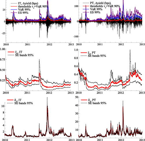
As was clear from Table 2, the coefficients $c^{\xi }$ and $c^{\delta }$ measure the impact of bond purchases on the tail behavior of yield changes. As these parameters are difficult to interpret by themselves, we show in Web Appendix L how they can be translated into an impact on VaR via their link to τ_t, δ_t, and ξ_t. For Italy, we obtain a total VaR impact of 0.0 (tail threshold) +0.8 (tail scale) – 5.9 (tail shape) = –5.1 bps for a €1 bn Eurosystem intervention. For Portugal, we obtain a larger impact of –0.1 (tail threshold) – 172.5 (tail scale) – 176.4 (tail shape) = –349.0 bps. These point estimates are of course subject to substantial estimation uncertainty; see Table 2. The 95% confidence intervals for VaR impact can be bootstrapped along with the parameters. They equal [–17.6, 11.6] for IT and [–664.0, –38.8] for PT. The stronger impact for Portugal than for Italy is likely due to a €1 bn intervention constituting a larger share of the overall market.

5 Conclusion

We introduced a semiparametric modeling framework to study time variation in tail parameters for long univariate time series. To this end we modeled the time variation in the shape and scale parameters of the Generalized Pareto Distribution, which approximates the tail of most heavy-tailed densities used in econometrics and the actuarial sciences. We discussed the handling of nontail time series observations, inference on deterministic and time-varying parameters, and how to relate tail variation to observed covariates if such variables are available. We also established conditions for stationarity and ergodicity of the model and conditions for consistency and asymptotic normality of the maximum likelihood estimator. The model therefore complements and extends recent work based on different methodologies, such as the nonparametric approach to tail index variation of de Haan and Zhou (2021), the time-varying quantile (and ES) approaches of Patton, Ziegel, and Chen (2019) and Catania and Luati (in press), and the parametric approach of Massacci (2017). We applied the model to study variation in the left tail of U.S. equity log-returns, and in the right tail of changes in euro area sovereign bond yields at a high frequency. In the latter case we also studied the impact of Eurosystem bond purchases, concluding that these had a beneficial impact on tail parameters, leaning against the risk of extremely adverse market outcomes.

Evidently, our model for time-varying tail parameters is focussed on capturing marginal features. In many applications it may also be of interest to study the time-varying nature of joint extremes; see for example, Castro-Camilo, de Carvalho, and Wadsworth (2018), Escobar-Bach et al. (2018), and Mhalla, de Carvalho, and Chavez-Demoulin (2019). In terms of our first illustration, for example, one could wonder whether extremely negative log-returns for the S&P 500 and IBM stock were more dependent at certain points in time. We leave such research for future work (see also Lucas, Schwaab, and Zhang, 2014; Oh and Patton, 2018; Hautsch and Herrera, 2020).

Supplementary Materials

Supplementary materials contain proofs and technical details, additional simulation and empirical results, and computer code (language: Ox) for the implementation of the method. The latter is also obtainable via www.gasmodel.com.

Acknowledgments

The views expressed in this article are those of the authors and do not necessarily reflect the views or policies of the BIS, the European Central Bank or Sveriges Riksbank.

Disclosure Statement

The authors report there are no competing interests to declare.

Notes

1 The web appendix considers additional applications to exchange rates and commodity prices.

2 Alternatively, one could opt to not update $f_t$ at all until a new $x_t>0$ arrives. Empirically, both approaches seem to work equally well.

3 See for instance Boswijk et al. (2021).

4 Web Appendix I provides two additional illustrations to other asset classes: exchange rates (GBP/USD) and commodities (Brent crude oil).

References

- Blasques, F., Koopman, S. J., and Lucas, A. (2015), “Information Theoretic Optimality of Observation Driven Time Series Models for Continuous Responses,” Biometrika, 102, 325–343. DOI: 10.1093/biomet/asu076.
- Blasques, F., van Brummelen, J., Koopman, S. J., and Lucas, A. (2022), “Maximum Likelihood Estimation for Generalized Autoregressive Score Models,” Journal of Econometrics, 227, 325–346. DOI: 10.1016/j.jeconom.2021.06.003.
- Boswijk, H. P., Cavaliere, G., Georgiev, I., and Rahbek, A. (2021), “Bootstrapping Non-stationary Stochastic Volatility,” Journal of Econometrics, 224, 161–180. DOI: 10.1016/j.jeconom.2021.01.005.
- Bougerol, P. (1993), “Kalman Filtering with Random Coefficients and Contractions,” SIAM Journal on Control and Optimization, 31, 942–959. DOI: 10.1137/0331041.
- Castro-Camilo, D., de Carvalho, M., and Wadsworth, J. (2018), “Time-Varying Extreme Value Dependence with Application to Leading European Stock Markets,” Annals of Applied Statistics, 12, 283–309.
- Catania, L., and Luati, A. (in press), “Semiparametric Modeling of Multiple Quantiles,” Journal of Econometrics.
- Chavez-Demoulin, V., Embrechts, P., and Sardy, S. (2014), “Extreme-Quantile Tracking for Financial Time Series,” Journal of Econometrics, 181, 44–52. DOI: 10.1016/j.jeconom.2014.02.007.
- Coles, S. (2001), An Introduction to Statistical Modeling of Extreme Values, London: Springer Press.
- Cox, D. R. (1981), “Statistical Analysis of Time Series: Some Recent Developments,” Scandinavian Journal of Statistics, 8, 93–115.
- Creal, D., Koopman, S. J., and Lucas, A. (2013), “Generalized Autoregressive Score Models with Applications,” Journal of Applied Econometrics, 28, 777–795. DOI: 10.1002/jae.1279.
- Creal, D., Schwaab, B., Koopman, S. J., and Lucas, A. (2014), “An Observation Driven Mixed Measurement Dynamic Factor Model with Application to Credit Risk,” The Review of Economics and Statistics, 96, 898915. DOI: 10.1162/REST_a_00393.
- Davidson, A. C., and Smith, R. L. (1990), “Models for Exceedances over High Thresholds,” Journal of the Royal Statistical Association, Series B, 52, 393–442. DOI: 10.1111/j.2517-6161.1990.tb01796.x.
- de Haan, L., and Zhou, C. (2021), “Trends in Extreme Value Indices,” Journal of the Americal Statistical Association, 116, 1265–1279. DOI: 10.1080/01621459.2019.1705307.
- Einmahl, J., de Haan, L., and Zhou, C. (2016), “Statistics of Heteroscedastic Extremes,” Journal of the Royal Statistical Society, Series B, 78, 31–51. DOI: 10.1111/rssb.12099.
- Embrechts, P., Klüppelberg, C., and Mikosch, T. (1997), Modelling Extremal Events for Insurance and Finance, Berlin: Springer Verlag.
- Engle, R. F., and Manganelli, S. (2004), “CAViaR: Conditional Autoregressive Value at Risk by Regression Quantiles,” Journal of Business & Economic Statistics, 22, 367–381. DOI: 10.1198/073500104000000370.
- Escobar-Bach, M., Goegebeur, Y., and Guillou, A. (2018), “Local Robust Estimation of the Pickands Dependence Function,” Annals of Statistics, 46, 2806–2843.
- Eser, F., and Schwaab, B. (2016), “Evaluating the Impact of Unconventional Monetary Policy Measures: Empirical Evidence from the ECB’s Securities Markets Programme,” Journal of Financial Economics, 119, 147–167. DOI: 10.1016/j.jfineco.2015.06.003.
- Galbraith, J. W., and Zernov, S. (2004), “Circuit Breakers and the Tail Index of Equity Returns,” Journal of Financial Econometrics, 2, 109–129. DOI: 10.1093/jjfinec/nbh005.
- Ghysels, E., Idier, J., Manganelli, S., and Vergote, O. (2017), “A High Frequency Assessment of the ECB Securities Markets Programme,” Journal of European Economic Association, 15, 218–243. DOI: 10.1093/jeea/jvw003.
- Hafner, C. M., and Wang, L. (in press), “A Dynamic Conditional Score Model for the Log Correlation Matrix,” Journal of Econometrics.
- Harvey, A. C. (2013), Dynamic Models for Volatility and Heavy Tails with Applications to Financial and Economic Time Series, Cambridge: Cambridge University Press.
- Hautsch, N., and Herrera, R. (2020), “Multivariate Dynamic Intensity Peaks-Over-Threshold Models,” Journal of Applied Econometrics, 35, 248–272. DOI: 10.1002/jae.2741.
- Hetland, S., Pedersen, R. S., and Rahbek, A. (in press), “Dynamic Conditional Eigenvalue GARCH,” Journal of Econometrics.
- Hill, B. (1975), “A Simple General Approach to Inference About the Tail of a Distribution,” The Annals of Statistics, 3, 1163–1174. DOI: 10.1214/aos/1176343247.
- Hoga, Y. (2017), “Testing for Changes in (Extreme) VaR,” Econometrics Journal, 20, 23–51. DOI: 10.1111/ectj.12080.
- Huisman, R., Koedijk, K., Kool, C., and Palm, F. (2001), “Tail-Index Estimates in Small Samples,” Journal of Business & Economic Statistics, 19, 208–216. DOI: 10.1198/073500101316970421.
- Jensen, S. T., and Rahbek, A. (2004), “Asymptotic Inference for Nonstationary GARCH,” Econometric Theory, 20, 1203–1226. DOI: 10.1017/S0266466604206065.
- Johnson, N. L., Kotz, S., and Balakrishnan, N. (1994), Continuous Univariate Distributions (Vol. 1, 2nd ed.), New York: Wiley.
- Koenker, R. (2005), Quantile Regression, Cambridge: Cambridge University Press.
- Lin, C.-H., and Kao, T.-C. (2018), “Multiple Structural Changes in the Tail Behavior: Evidence from Stock Market Futures Returns,” Nonlinear Analysis: Real World Applications, 9, 1702–1713. DOI: 10.1016/j.nonrwa.2007.05.011.
- Lucas, A., Schwaab, B., and Zhang, X. (2014), “Conditional Euro Area Sovereign Default Risk,” Journal of Business and Economics Statistics, 32, 271–284. DOI: 10.1080/07350015.2013.873540.
- Lucas, A., and Zhang, X. (2016), “Score Driven Exponentially Weighted Moving Average and Value-at-Risk Forecasting,” International Journal of Forecasting, 32, 293–302. DOI: 10.1016/j.ijforecast.2015.09.003.
- Massacci, D. (2017), “Tail Risk Dynamics in Stock Returns: Links to the Macroeconomy and Global Markets Connectedness,” Management Science, 63, 112–132. DOI: 10.1287/mnsc.2016.2488.
- McNeil, A., and Frey, R. (2000), “Estimation of Tail-Related Risk Measures for Heteroscedastic Financial Time Series: An Extreme Value Approach,” Journal of Empirical Finance, 7, 271–300. DOI: 10.1016/S0927-5398(00)00012-8.
- McNeil, A. J., Frey, R., and Embrechts, P. (2010), Quantitative Risk Management: Concepts, Techniques, and Tools, Princeton, NJ: Princeton University press.
- Mhalla, L., de Carvalho, M., and Chavez-Demoulin, V. (2019), “Regression-Type Models for Extremal Dependence,” Scandinavian Journal of Statistics, 46, 1141–1167. DOI: 10.1111/sjos.12388.
- Oh, D. H., and Patton, A. J. (2018), “Time-Varying Systemic Risk: Evidence from a Dynamic Copula Model of CDS Spreads,” Journal of Business & Economic Statistics, 36, 181–195. DOI: 10.1080/07350015.2016.1177535.
- Patton, A. (2006), “Modelling Asymmetric Exchange Rate Dependence,” International Economic Review, 47, 527–556. DOI: 10.1111/j.1468-2354.2006.00387.x.
- Patton, A. J., Ziegel, J. F., and Chen, R. (2019), “Dynamic Semiparametric Models for Expected Shortfall (and Value-at-Risk),” Journal of Econometrics, 211, 388–413. DOI: 10.1016/j.jeconom.2018.10.008.
- Quintos, C., Fan, Z., and Phillips, P. C. (2001), “Structural Change Tests in Tail Behaviour and the Asian Crisis,” The Review of Economic Studies, 68, 633–663. DOI: 10.1111/1467-937X.00184.
- Rocco, M. (2014), “Extreme Value Theory in Finance: A Survey,” Journal of Economic Surveys, 28, 82–108. DOI: 10.1111/j.1467-6419.2012.00744.x.
- Straumann, D., and Mikosch, T. (2006), “Quasi-Maximum-Likelihood Estimation in Conditionally Heteroscedastic Time Series: A Stochastic Recurrence Equations Approach,” The Annals of Statistics, 34, 2449–2495. DOI: 10.1214/009053606000000803.
- Wang, H., and Tsai, C.-L. (2009), “Tail Index Regression,” Journal of the American Statistical Association, 104, 1233–1240. DOI: 10.1198/jasa.2009.tm08458.
- Werner, T., and Upper, C. (2004), “Time Variation in the Tail Behavior of Bund Future Returns,” Journal of Futures Markets, 24, 387–398. DOI: 10.1002/fut.10120.