Bootstrap Inference in Cointegrating Regressions: Traditional and Self-Normalized Test Statistics

Abstract

Traditional tests of hypotheses on the cointegrating vector are well known to suffer from severe size distortions in finite samples, especially when the data are characterized by large levels of endogeneity or error serial correlation. To address this issue, we combine a vector autoregressive (VAR) sieve bootstrap to construct critical values with a self-normalization approach that avoids direct estimation of long-run variance parameters when computing test statistics. To asymptotically justify this method, we prove bootstrap consistency for the self-normalized test statistics under mild conditions. In addition, the underlying bootstrap invariance principle allows us to prove bootstrap consistency also for traditional test statistics based on popular modified OLS estimators. Simulation results show that using bootstrap critical values instead of asymptotic critical values reduces size distortions associated with traditional test statistics considerably, but combining the VAR sieve bootstrap with self-normalization can lead to even less size distorted tests at the cost of only small power losses. We illustrate the usefulness of the VAR sieve bootstrap in empirical applications by analyzing the validity of the Fisher effect in 19 OECD countries.

KEYWORDS:

• Bootstrap consistency
• Cointegration
• Self-normalization
• Sieve bootstrap
• Size distortions
• Tuning parameters

1 Introduction

Cointegration methods have been and are widely used to analyze long-run relationships between stochastically trending variables in many areas such as macroeconomics, environmental economics, and finance, see, for example, Benati et al. (2021), Wagner (2015), and Rad, Low, and Faff (2016) for recent examples. In addition to these classical fields of application, cointegration methods have recently proven to be useful to describe phenomena in physics (Dahlhaus, Kiss, and Neddermeyer 2018) and climate change (Phillips, Leirvik, and Storelvmo 2020).

It is standard practice in empirical applications to test linear restrictions on the cointegrating vector by means of traditional Wald-type test statistics based on a suitable consistent estimator of the cointegrating vector and on a nonparametric kernel estimator of a long-run variance parameter for standardization. In the presence of endogeneity, the limiting distribution of the OLS estimator is contaminated by second order bias terms making the estimator unsuitable for standard asymptotic inference. The literature provides several endogeneity corrected estimators with a zero-mean Gaussian mixture limiting distribution allowing for asymptotically valid inference based on Chi-squared critical values. The most popular estimators are the dynamic OLS (D-OLS) estimator (Phillips and Loretan 1991; Saikkonen 1991; Stock and Watson 1993), the fully modified OLS (FM-OLS) estimator (Phillips and Hansen 1990), and the integrated modified OLS (IM-OLS) estimator (Vogelsang and Wagner 2014). Tests based upon these estimators are implemented in several software packages and are thus easy to apply in applications. However, they are all well known to be severely size distorted in finite samples, especially when the data are characterized by large levels of endogeneity or error serial correlation. Similar problems are also observed for tests based on alternative estimators proposed in, for example, Phillips (2014) and Hwang and Sun (2018).

To address these size distortions, this article combines a vector autoregressive (VAR) sieve bootstrap to construct critical values with a self-normalization approach that avoids direct estimation of the long-run variance parameter when computing test statistics. In particular, we discuss three self-normalized Wald-type test statistics based on the tuning parameter free IM-OLS estimator, which do not rely on a consistent tuning parameter dependent long-run variance estimator but still possess a pivotal limiting distribution under the null hypothesis. The concept of self-normalization has been proven to be useful in the analysis of stationary time series (see, e.g., Kiefer, Vogelsang, and Bunzel 2000; Shao 2010a, 2015) but has not received much attention in the cointegrating regression literature as an alternative to traditional test statistics. As we will see in Section 3, self-normalization is closely related to, but does not need to be a special case of, the fixed-b approach of Vogelsang and Wagner (2014).

In contrast, the nowadays classical VAR sieve bootstrap (Kreiss 1992; Paparoditis 1996; Bühlmann 1997) has already been applied to cointegrating regressions in various setups. Psaradakis (2001), inspired by the seminal work of Li and Maddala (1997), shows the superior performance when VAR sieve bootstrap critical values replace Chi-squared critical values for the traditional Wald-type test based on the FM-OLS estimator (without asymptotically justifying the approach). Park (2002) proves an invariance principle for the bootstrap process under the assumption that the errors form a linear process with iid innovations. The invariance principle allows Chang, Park, and Song (2006) to prove consistency of the VAR sieve bootstrap for the traditional Wald-type test statistic based on the D-OLS estimator. Although the bootstrap leads to considerable performance advantages over the tests based on asymptotic critical values, it is rarely used in empirical applications.

Alternative bootstrap approaches studied in the cointegrating regression literature are the stationary bootstrap (SB) of Politis and Romano (1994) and the residual-based block bootstrap (RBB) of Paparoditis and Politis (2003), which have been proven to be consistent for the limiting distribution of the OLS estimator of the cointegrating vector in Shin and Hwang (2013) and Jentsch, Politis, and Paparoditis (2015), respectively. Moreover, the dependent wild bootstrap (DWB) of Shao (2010b) has been proven to be useful when testing for unit roots (Rho and Shao 2019), but has not been asymptotically justified in cointegrating regressions yet. In contrast to selecting the order of the VAR sieve for the VAR sieve bootstrap, however, choosing a suitable geometric distribution for the SB, a suitable block size for the RBB, or a suitable combination of kernel and bandwidth for the DWB seem to be rather challenging tasks in empirical applications.

To prove consistency of the VAR sieve bootstrap for the self-normalized test statistics, we derive a bootstrap invariance principle under mild conditions. In particular, in contrast to Park (2002) and Chang, Park, and Song (2006), we allow for uncorrelated but not necessarily independent white noise innovations. The bootstrap invariance principle might thus be of independent interest. In addition, it allows us to prove bootstrap consistency also for the traditional Wald-type test statistics based on the D-OLS, FM-OLS, and IM-OLS estimators. With respect to the traditional Wald-type test statistic based on the D-OLS estimator, this article thus extends the results in Chang, Park, and Song (2006). Finally, we emphasize that one of the self-normalized test statistics proposed in this article has a pivotal limiting null distribution only in case the number of linearly independent restrictions on the cointegrating vector is equal to the dimension of the cointegrating vector. Thus, for this particular test statistic, the VAR sieve bootstrap is key to allow for asymptotically valid inference also for a smaller number of linearly independent restrictions on the cointegrating vector.

The theoretical analysis is complemented by a detailed simulation study analyzing local asymptotic power of the tests and assessing test performance in finite samples. The results reveal tremendous performance advantages of traditional tests based on bootstrap critical values over those based on Chi-squared critical values. In addition, we find that the self-normalized tests based on asymptotic critical values are considerably less size distorted than the traditional tests based on asymptotic critical values for small to medium levels of endogeneity and error serial correlation at the cost of only small power losses under the alternative. For large levels of endogeneity and error serial correlation, however, self-normalization alone is less advantageous. In these cases, the VAR sieve bootstrap improves the performance of the self-normalized tests considerably, with two of the self-normalized tests often outperforming the traditional tests based on bootstrap critical values.

Finally, we demonstrate the usefulness of the VAR sieve bootstrap in applications by analyzing the validity of the Fisher effect in 19 OECD countries in the three decades prior to the Covid-19 crisis. The Fisher effect states that inflation and the short-term nominal interest rate are in a one-for-one relationship. It is backed by many theoretical models but often rejected in empirical studies, possibly because of the poor performance of estimators and tests in the presence of highly persistent errors typically observed in Fisher equations (Caporale and Pittis 2004; Westerlund 2008). Indeed, we find that the traditional and self-normalized tests based on asymptotic critical values tend to reject the Fisher effect for several countries, whereas the tests based on bootstrap critical values indicate the validity of the Fisher effect for almost all countries under consideration.

The article proceeds as follows: Section 2 introduces the model and its underlying assumptions. Section 3 reviews the IM-OLS approach and proposes three self-normalized test statistics based upon it. Section 4 presents the VAR sieve bootstrap procedure for the self-normalized test statistics and popular traditional test statistics and proves its asymptotic validity in each case. Section 5 contains the simulation study and Section 6 is devoted to the empirical illustration. Section 7 summarizes and concludes. All proofs as well as additional supplementary materials are relegated to the Online Appendix.

Notation: $\lfloor x\rfloor$ denotes the integer part of $x\in \mathbb{R},|A{|}_F={(\text{tr}(A\prime A))}^{1/2}$ denotes the Frobenius norm of a real matrix A, and $\text{diag}(·)$ denotes a (block) diagonal matrix with diagonal elements specified throughout. With $\stackrel{w}{\to }$ and $\stackrel{p}{\to }$ we denote weak convergence and convergence in probability, respectively, as $T\to \infty$, with $\mathbb{P}$ denoting the underlying probability measure. Convergence in the bootstrap probability space is denoted by $\stackrel{w^{*}}{\to }$ and $\stackrel{p^{*}}{\to }$, with ${\mathbb{P}}^{*}$ denoting the corresponding probability measure (conditional on the data) and ${\mathbb{E}}^{*}(·)$ denoting the expectation with respect to ${\mathbb{P}}^{*}$. Throughout, random variables in the bootstrap probability space are indicated by the superscript “$*$”.

2 The Model and Assumptions

We consider the cointegrating regression model (1) $$y_t=x_t^{\prime }\beta +u_t,$$(1) (2) $$x_t=x_{t-1}+v_t,$$(2) for observations $t=1,\dots ,T$, where y_t is a scalar time series and x_t is an $m\times 1$ vector of time series. For notational brevity, we set $x_0=0$ and exclude deterministic components from (1). Nevertheless, incorporating deterministic components (fulfilling the condition in eq. (14)(14) $${\tau }_{\text{IM}}({\widehat{\eta }}^{\perp })\stackrel{w}{\to }\frac{{\chi }_s^2}{{\int }_0^1{\left(W_{u·v}(r)-h(r)\prime Q\right)}^{2}dr}=:{\mathcal{G}}_{\text{SN}}^{\perp },$$(14) in Vogelsang and Wagner 2014) is straightforward and the accompanying software code allows to handle the more general case. To derive asymptotic theory, we have to impose assumptions on the process ${\left\{w_t\right\}}_{t\in \mathbb{Z}}:={\{[u_t,v_t^{\prime }]\prime \}}_{t\in \mathbb{Z}}$.

Assumption 1

Let ${\left\{w_t\right\}}_{t\in \mathbb{Z}}$ be an ${\mathbb{R}}^{1+m}$-valued, strictly stationary, and purely nondeterministic stochastic process of full rank with $\mathbb{E}(w_t)=0$ and $\mathbb{E}(|w_t{|}_F^a)<\infty$ for some a > 2. The autocovariance matrix function $\Gamma (·)$ of ${\left\{w_t\right\}}_{t\in \mathbb{Z}}$ fulfills ${\sum }_{h=-\infty }^{\infty }{(1+|h|)}^k|\Gamma (h){|}_F<\infty$ for some $k\ge 3/2$. For the spectral density matrix $f(·)$ of ${\left\{w_t\right\}}_{t\in \mathbb{Z}}$ there exists a constant c > 0 such that $\min \sigma (f(\lambda ))\ge c$ for all frequencies $\lambda \in (-\pi ,\pi ]$, where $\sigma (f(\lambda ))$ denotes the spectrum of $f(·)$ at frequency λ.

Assumption 1 is similar to Assumption (A) in Meyer and Kreiss (2015). The parameter k controls the convergence rate of the VAR sieve approximation, compare eq. (E.3) in Online Appendix E and Remark 3.3 in Meyer and Kreiss (2015). The short memory condition in Assumption 1 implies that f is continuously differentiable and bounded from below and from above, uniformly for all frequencies $\lambda \in (-\pi ,\pi ]$. As shown in Meyer and Kreiss (2015), a process fulfilling Assumption 1 always possesses the one-sided representations (3) $$\Phi (L)w_t={\epsilon }_t\hspace{1em}\text{and}\hspace{1em}{w}_t=\Psi (L){\epsilon }_t,$$(3) where ${\left\{{\epsilon }_t\right\}}_{t\in \mathbb{Z}}$ is a strictly stationary uncorrelated but not necessarily independent white noise process with positive definite covariance matrix Σ and L denotes the backward shift operator. For $\Phi (z):=I_{m+1}-{\sum }_{j=1}^{\infty }{\Phi }_j{z}^j$ and $\Psi (z):=I_{m+1}+{\sum }_{j=1}^{\infty }{\Psi }_j{z}^j$ it holds that $\text{det}(\Phi (z))\ne 0$ and $\text{det}(\Psi (z))\ne 0$ for all $\left|z\right|\le 1$ and ${\sum }_{j=1}^{\infty }{(1+j)}^k|{\Phi }_j{|}_F<\infty$ and ${\sum }_{j=1}^{\infty }{(1+j)}^k|{\Psi }_j{|}_F<\infty$ for the k from Assumption 1.

Assumption 2

The process ${\left\{w_t\right\}}_{t\in \mathbb{Z}}$ has absolutely summable cumulants up to order four. More precisely, it holds for all $j=2,\dots ,4$ and $a=[a_1,\dots ,a_j]\prime \in {\{1,\dots ,m+1\}}^j$, that ${\sum }_{h_2,\dots ,h_j=-\infty }^{\infty }|{\text{cum}}_a(0,h_2,\dots ,h_j)|<\infty$, where ${\text{cum}}_a(0,h_2,\dots ,h_j)$ denotes the jth joint cumulant of $w_{a_1,0},$ $w_{a_2,h_2},\dots ,w_{a_j,h_j}$ and $w_{i,t}$ denotes the ith element of w_t (see, e.g., Brillinger 1981).

Let Ω denote the long-run covariance matrix of ${\left\{w_t\right\}}_{t\in \mathbb{Z}}$, that is, $$\begin{array}{c}\Omega =\left[\begin{array}{cc}{\Omega }_{uu}& {\Omega }_{uv}\\ {\Omega }_{vu}& {\Omega }_{vv}\end{array}\right]=2\pi f(0)=\sum _{h=-\infty }^{\infty }\mathbb{E}(w_0{w}_h^{\prime })\\ =\Psi (1)\Sigma \Psi (1)\prime .\end{array}$$

From $\Sigma >0$ and $\text{det}(\Psi (1))\ne 0$ it follows that $\Omega >0$, which, in particular, excludes cointegration among the elements of x_t. For later usage, we also define the one-sided long-run covariance matrix $\Delta :={\sum }_{h=0}^{\infty }\mathbb{E}(w_0{w}_h^{\prime })$ and partition it analogously to Ω. Finally, we assume an invariance principle to hold for ${\left\{w_t\right\}}_{t\in \mathbb{Z}}$.

Assumption 3

Let ${\left\{w_t\right\}}_{t\in \mathbb{Z}}$ fulfill (4) $$\begin{array}{c}{B}_T(r):=T^{-1/2}\sum _{t=1}^{\lfloor rT\rfloor }{w}_t\stackrel{w}{\to }B(r)=\left[\begin{array}{c}{B}_u(r)\\ B_v(r)\end{array}\right]\\ ={\Omega }^{1/2}W(r),\hspace{1em}0\le r\le 1,\end{array}$$(4) where $W(r)=[W_{u·v}(r),W_v(r)\prime ]\prime$ is an $(1+m)$-dimensional vector of independent standard Brownian motions.

In the following, it is convenient to work with ${\Omega }^{1/2}$ of the form $${\Omega }^{1/2}=\left[\begin{array}{cc}{\Omega }_{u·v}^{1/2}& {\Omega }_{uv}({\Omega }_{vv}^{-1/2})\prime \\ 0& {\Omega }_{vv}^{1/2}\end{array}\right],$$such that ${\Omega }^{1/2}({\Omega }^{1/2})\prime =\Omega$, where ${\Omega }_{u·v}:={\Omega }_{uu}-{\Omega }_{uv}{\Omega }_{vv}^{-1}{\Omega }_{vu}$ is the variance of the scalar Brownian motion $B_{u·v}(r):=B_u(r)-B_v(r)\prime {\Omega }_{vv}^{-1}{\Omega }_{vu}$.

In contrast to the assumptions in Park (2002) and Chang, Park, and Song (2006), Assumption 1 does explicitly not ask for invertibility or causality of the process ${\left\{w_t\right\}}_{t\in \mathbb{Z}}$ with respect to an independent white noise process. Instead, in this article, the process ${\left\{{\epsilon }_t\right\}}_{t\in \mathbb{Z}}$ is an uncorrelated but not necessarily independent white noise process. When working with macroeconomic and financial time series, an important deviation from independence is conditional heteroscedasticity (see, e.g., Engle 1982; Gonçalves and Kilian 2004). In particular, when analyzing the Fisher effect in Section 6, it may be natural to allow for conditional heteroscedasticity, as parts of the literature provide empirical evidence that the level of inflation affects its volatility (see, e.g., Baillie, Chung, and Tieslau 1996). Our set of assumptions allows for unknown forms of conditional heteroscedasticity (see, e.g., Brüggemann, Jentsch, and Trenkler 2016) in ${\left\{w_t\right\}}_{t\in \mathbb{Z}}$ and covers, for example, linear processes with generalized autoregressive conditional heteroscedastic (GARCH) innovations (Bollerslev 1986), studied in detail in Wu and Min (2005) and also covered by the assumptions in, for example, Kuersteiner (2001) and Gonçalves and Kilian (2004, 2007). We also employ GARCH processes to introduce conditional heteroscedasticity into the data generating processes considered in the Monte Carlo simulations in Section 5.2.

3 Self-Normalized Test Statistics

It is standard practice in applications to test $s\le m$ linearly independent restrictions on $\beta \in {\mathbb{R}}^m$ in (1) of the form ${\mathrm{H}}_0: R_1\beta =r_0$ versus ${\mathrm{H}}_1: R_1\beta \ne r_0$ by means of traditional Wald-type test statistics, where $R_1\in {\mathbb{R}}^{s\times m}$ has full row rank s and $r_0\in {\mathbb{R}}^s$. Using generic notation, traditional Wald-type test statistics are defined as (5) $$\tau ({\widehat{\Omega }}_{u·v}):=\left(R_1\widehat{\beta }-r_0\right)\prime {\left[R_1{\widehat{\Omega }}_{u·v}\widehat{V}{R}_1^{\prime }\right]}^{-1}\left(R_1\widehat{\beta }-r_0\right),$$(5) where $\widehat{\beta }$ is an estimator of β whose limiting distribution is a zero-mean Gaussian mixture (e. g., the D-OLS, FM-OLS, or IM-OLS estimator), $\widehat{V}$ is the unscaled sample covariance matrix of $\widehat{\beta }$, and ${\widehat{\Omega }}_{u·v}:={\widehat{\Omega }}_{uu}-{\widehat{\Omega }}_{uv}{\widehat{\Omega }}_{vv}^{-1}{\widehat{\Omega }}_{vu}$ is a consistent estimator of ${\Omega }_{u·v}$. The (block) elements of Ω are typically estimated based on the OLS residuals ${\widehat{u}}_{\text{OLS},t}$ in (1) and the first differences of x_t using a nonparametric kernel estimator of the form (6) $$\begin{array}{c}\widehat{\Omega }=\left[\begin{array}{cc}{\widehat{\Omega }}_{uu}& {\widehat{\Omega }}_{uv}\\ {\widehat{\Omega }}_{vu}& {\widehat{\Omega }}_{vv}\end{array}\right]\\ :=T^{-1}\sum _{i=1}^T\sum _{j=1}^T\mathcal{K}\left(\frac{|i-j|}{b_T}\right)\left[\begin{array}{c}{\widehat{u}}_{\text{OLS},i}\\ v_i\end{array}\right]\left[\begin{array}{c}{\widehat{u}}_{\text{OLS},j}\\ v_j\end{array}\right]\prime ,\end{array}$$(6) where $\mathcal{K}(·)$ denotes a kernel weighting function and b_T a bandwidth parameter fulfilling some technical conditions (see e.g., Jansson 2002).

These traditional test statistics are asymptotically Chi-squared distributed with s degrees of freedom (denoted as ${\chi }_s^2$ in the following). However, it is well known in the literature that the tests suffer from severe size distortions in finite samples, especially when the data are characterized by large levels of endogeneity or error serial correlation. Clearly, these size distortions are explained by the poor approximation quality of the Chi-squared distribution to the finite sample distributions of the traditional test statistics in these cases.

One reason for this poor approximation quality are finite sample effects of tuning parameter choices required for estimating ${\Omega }_{u·v}$ and—unless the tuning parameter free IM-OLS approach of Vogelsang and Wagner (2014) is used—also β on the finite sample distribution of traditional test statistics. Therefore, Vogelsang and Wagner (2014) propose a fixed-b approach based on the IM-OLS estimator, which allows to tabulate critical values corresponding to the kernel and bandwidth choices made when estimating ${\Omega }_{u·v}$. However, simulation results in Vogelsang and Wagner (2014) reveal that the performance of the test is still sensitive to the choice of $b=b_T/T$ $\in (0,1]$.

A promising alternative approach is the concept of self-normalization, which has not received much attention in the cointegrating regression literature as an alternative to traditional test statistics. The main idea of self-normalization is to replace a tuning parameter dependent estimator of a long-run variance parameter in the construction of a test statistic with a quantity that is asymptotically proportional to this particular long-run variance parameter and can be directly computed from the data without requiring tuning parameter choices (Shao 2010a).

Because its construction is completely tuning parameter free, the IM-OLS estimator of Vogelsang and Wagner (2014) serves as a natural starting point for developing self-normalized Wald-type test statistics in cointegrating regressions. For completeness, let us briefly review the IM-OLS approach. The IM-OLS estimator ${\widehat{\beta }}_{\text{IM}}$ of β in (1) is defined as the OLS estimator of β in the augmented partial sums regression (7) $$S_t^y=S_t^{x\prime }\beta +x_t^{\prime }\gamma +S_t^u=Z_t^{\prime }\theta +S_t^u,$$(7) where $S_t^y:={\sum }_{s=1}^t{y}_s,S_t^x:={\sum }_{s=1}^t{x}_s,S_t^u:={\sum }_{s=1}^t{u}_s,Z_t:=[S_t^{x\prime },x_t^{\prime }]\prime$, and $\theta :=[\beta \prime ,\gamma \prime ]\prime$. Adding x_t to the partial sums regression serves as an endogeneity correction, which is similar in spirit to the leads and lags augmentation in D-OLS estimation but avoids tuning parameter choices. Denoting the OLS estimator of θ in (7) with ${\widehat{\theta }}_{\text{IM}}:=[{\widehat{\beta }}_{\text{IM}}^{\prime },{\widehat{\gamma }}_{\text{IM}}^{\prime }]\prime$, (Vogelsang and Wagner 2014, Theorem 2) show that it holds under Assumption 3 that the limiting distribution of ${\widehat{\theta }}_{\text{IM}}$ is given by (8) $$\left[\begin{array}{c}T\left({\widehat{\beta }}_{\text{IM}}-\beta \right)\\ {\widehat{\gamma }}_{\text{IM}}-{\Omega }_{vv}^{-1}{\Omega }_{vu}\end{array}\right]\stackrel{w}{\to }{\Omega }_{u·v}^{1/2}{\left(\Pi \prime \right)}^{-1}\mathcal{Z},$$(8) where $\Pi :=\text{diag}({\Omega }_{vv}^{1/2},{\Omega }_{vv}^{1/2})$, $\mathcal{Z}:={({\int }_0^{1}g(r)g(r)\prime dr)}^{-1}{\int }_0^1$ $\left[G(1)-G(r)\right]d{W}_{u·v}(r),g(r):=[{\int }_0^r{W}_v(s)\prime ds,W_v(r)\prime ]\prime$, and $G(r):={\int }_0^{r}g(s)ds$. As both x_t and $S_t^u$ are integrated processes, the correlation between $B_v(r)$ and $B_u(r)$ is soaked up in the long-run population regression vector ${\Omega }_{vv}^{-1}{\Omega }_{vu}$. Therefore, as Vogelsang and Wagner (2014) point out, the correct centering parameter for ${\widehat{\gamma }}_{\text{IM}}$ in the presence of endogeneity is ${\Omega }_{vv}^{-1}{\Omega }_{vu}$ rather than the population value γ = 0. Conditional upon $W_v(r)$, the limiting distribution in (8) is Gaussian with zero-mean and covariance matrix ${\Omega }_{u·v}{V}_{\text{IM}}$, where $V_{\text{IM}}={(\Pi \prime )}^{-1}{\tilde{V}}_{\text{IM}}{\Pi }^{-1}$ and $$\begin{array}{c}{\tilde{V}}_{\text{IM}}:={\left({\int }_0^{1}g(r)g(r)\prime dr\right)}^{-1}({\int }_0^1\left[G(1)-G(r)\right]\\ \hspace{1em}\times \left[G(1)-G(r)\right]\prime dr){\left({\int }_0^{1}g(r)g(r)\prime dr\right)}^{-1}.\end{array}$$

The traditional Wald-type test statistic based on the IM-OLS estimator, in the following denoted by ${\tau }_{\text{IM}}({\widehat{\Omega }}_{u·v})$, is thus given by $\tau ({\widehat{\Omega }}_{u·v})$ as defined in (5), with $\widehat{\beta }={\widehat{\beta }}_{\text{IM}}^{\prime }$ and $\widehat{V}$ equal to the upper left (m × m)-dimensional block element of the ($2m\times 2m$)-dimensional matrix (9) $${\widehat{V}}_{\text{IM}}:={\left(\sum _{t=1}^T{Z}_t{Z}_t^{\prime }\right)}^{-1}\left(\sum _{t=1}^T{c}_t{c}_t^{\prime }\right){\left(\sum _{t=1}^T{Z}_t{Z}_t^{\prime }\right)}^{-1},$$(9) where $c_1:=S_T^Z$ and $c_t:=S_T^Z-S_{t-1}^Z$, with $S_t^Z:={\sum }_{j=1}^t{Z}_j$, for $t=2,\dots ,T$. For later usage, Online Appendix B reviews the construction of the traditional Wald-type test statistics based on the D-OLS and FM-OLS estimators, in the following denoted by ${\tau }_{\mathrm{D}}({\widehat{\Omega }}_{u·v})$ and ${\tau }_{\text{FM}}({\widehat{\Omega }}_{u·v})$, respectively.

We now proceed with the construction of a self-normalized test statistic based on the IM-OLS estimator. To simplify the expression of asymptotic results, let us rewrite the null hypothesis in terms of the correct centering parameter for ${\widehat{\theta }}_{\text{IM}}$, given by $[\beta \prime ,({\Omega }_{vv}^{-1}{\Omega }_{vu})\prime ]\prime$. To this end, define $R_2:=[R_1,0_{s\times m}]\in {\mathbb{R}}^{s\times 2m}$ such that the null hypothesis reads as $R_1\beta =R_2[\beta \prime ,({\Omega }_{vv}^{-1}{\Omega }_{vu})\prime ]\prime =r_0$. Clearly, the auxiliary coefficient vector γ is not restricted under the null hypothesis and, in particular, ${\Omega }_{vv}^{-1}{\Omega }_{vu}$ does not need to be estimated. Moreover, define (10) $${\tau }_{\text{IM}}(\kappa ):=\left(R_2{\widehat{\theta }}_{\text{IM}}-r_0\right)\prime {\left[R_2\kappa {\widehat{V}}_{\text{IM}}{R}_2^{\prime }\right]}^{-1}\left(R_2{\widehat{\theta }}_{\text{IM}}-r_0\right),$$(10) which coincides with the traditional Wald-type test statistic based on the IM-OLS estimator in case $\kappa ={\widehat{\Omega }}_{u·v}$. Inspired by Kiefer, Vogelsang, and Bunzel (2000), a straightforward choice for the self-normalizer is given by $\widehat{\eta }:=T^{-2}{\sum }_{t=2}^T{({\sum }_{s=2}^t\Delta {\widehat{S}}_s^u)}^2$, where $\Delta {\widehat{S}}_t^u:={\widehat{S}}_t^u-{\widehat{S}}_{t-1}^u$, $t=2,\dots ,T$, are the first differences of the OLS residuals ${\widehat{S}}_t^u:=S_t^y-Z_t^{\prime }{\widehat{\theta }}_{\text{IM}}$ in the augmented partial sums regression (7). The proof of Proposition 1 reveals that the self-normalizer converges weakly to ${\Omega }_{u·v}{\int }_0^1{(W_{u·v}(r)-g(r)\prime \mathcal{Z})}^{2}dr$, that is, its limiting distribution is scale dependent on ${\Omega }_{u·v}$. Choosing $\kappa =\widehat{\eta }$ in (10) thus removes the nuisance parameter ${\Omega }_{u·v}$ asymptotically, without estimating it directly. The resulting test statistic is closely related to, but not a special case of, the $\tilde{W}$ statistic considered in Vogelsang and Wagner (2014), compare the discussion in Remark 2.

Proposition 1.

Let the data be generated by (1) and (2) and let ${\left\{w_t\right\}}_{t\in \mathbb{Z}}$ satisfy Assumption 3. Then, under the null hypothesis, it holds that (11) $$\begin{array}{c}{\tau }_{\text{IM}}(\widehat{\eta })\stackrel{w}{\to }\frac{\left(R_2{\left(\Pi \prime \right)}^{-1}\mathcal{Z}\right)\prime {\left(R_2{V}_{\text{IM}}{R}_2^{\prime }\right)}^{-1}\left(R_2{\left(\Pi \prime \right)}^{-1}\mathcal{Z}\right)}{{\int }_0^1{\left(W_{u·v}(r)-g(r)\prime \mathcal{Z}\right)}^{2}dr}\\ =:{\mathcal{G}}_{\text{SN}}.\end{array}$$(11)

The limiting null distribution in Proposition 1 is a ratio of two random variables. It is straightforward to verify that the marginal distribution of the numerator is ${\chi }_s^2$, while the marginal distribution of the denominator is nonstandard but free of any nuisance parameters. However, it follows from (Vogelsang and Wagner 2014, Lemma 2) that numerator and denominator are correlated with the correlation depending on nuisance parameters through Π. Hence, tabulating asymptotically valid critical values for ${\tau }_{\text{IM}}(\widehat{\eta })$ is not possible in general.

Remark 1.

In the special case where the number of linearly independent restrictions on β equals the dimension of β (i. e., in case s = m), it follows from the definition of R₂, invertibility of R₁, and simple algebra that $$\begin{array}{c}\left(R_2{\left(\Pi \prime \right)}^{-1}\mathcal{Z}\right)\prime {\left(R_2{V}_{\text{IM}}{R}_2^{\prime }\right)}^{-1}\left(R_2{\left(\Pi \prime \right)}^{-1}\mathcal{Z}\right)\\ =\mathcal{Z}(1)\prime {\tilde{V}}_{\text{IM}}{(1,1)}^{-1}\mathcal{Z}(1),\end{array}$$where ${\tilde{V}}_{\text{IM}}(1,1)$ denotes the upper left (m × m)-dimensional block element of the ($2m\times 2m$)-dimensional matrix ${\tilde{V}}_{\text{IM}}$ and $\mathcal{Z}(1)$ denotes the vector of the first m elements of $\mathcal{Z}$. Thus, R₂ and Π cancel out algebraically and the correlation between numerator and denominator of the limiting distribution in (11) becomes nuisance parameter free. Table A.1 in Online Appendix A provides asymptotically valid critical values for ${\tau }_{\text{IM}}(\widehat{\eta })$ in case s = m for $m=1,\dots ,4$.

Table 1 Empirical sizes of the tests for ${\mathrm{H}}_0: {\beta }_1=1, {\beta }_2=1$ at 5% level based on asymptotic critical values.

						Traditional tests
			Self-normalized tests			Bartlett kernel			QS kernel			LR tests
$\varphi$	${\rho }_1,{\rho }_2$	${\tau }_{\text{OLS}}({\widehat{\sigma }}_u^2)$	${\tau }_{\text{IM}}({\tilde{\eta }}^{\perp })$	${\tau }_{\text{IM}}({\widehat{\eta }}^{\perp })$	${\tau }_{\text{IM}}(\widehat{\eta })$	${\tau }_{\mathrm{D}}({\widehat{\Omega }}_{u·v})$	${\tau }_{\text{FM}}({\widehat{\Omega }}_{u·v})$	${\tau }_{\text{IM}}({\widehat{\Omega }}_{u·v})$	${\tau }_{\mathrm{D}}({\widehat{\Omega }}_{u·v})$	${\tau }_{\text{FM}}({\widehat{\Omega }}_{u·v})$	${\tau }_{\text{IM}}({\widehat{\Omega }}_{u·v})$	LR(AIC)	LR(BIC)
Panel A: T = 75
0	0	0.06	0.04	0.03	0.03	0.13	0.15	0.11	0.17	0.20	0.14	0.13	0.10
	0.3	0.25	0.08	0.05	0.05	0.15	0.21	0.14	0.15	0.23	0.14	0.14	0.15
	0.6	0.69	0.15	0.13	0.08	0.24	0.40	0.19	0.23	0.43	0.18	0.16	0.18
	0.9	0.97	0.66	0.75	0.36	0.42	0.83	0.69	0.54	0.88	0.77	0.27	0.25
0.3	0	0.16	0.06	0.04	0.04	0.15	0.18	0.13	0.17	0.21	0.15	0.14	0.11
	0.3	0.34	0.09	0.07	0.06	0.16	0.23	0.15	0.16	0.25	0.15	0.15	0.16
	0.6	0.69	0.16	0.15	0.09	0.25	0.41	0.22	0.27	0.44	0.23	0.19	0.18
	0.9	0.96	0.65	0.72	0.35	0.46	0.81	0.69	0.63	0.89	0.80	0.32	0.30
0.9	0	0.25	0.07	0.05	0.05	0.16	0.19	0.15	0.17	0.23	0.16	0.18	0.15
	0.3	0.39	0.10	0.08	0.07	0.20	0.26	0.18	0.22	0.30	0.19	0.20	0.17
	0.6	0.67	0.17	0.16	0.10	0.28	0.41	0.26	0.33	0.49	0.31	0.23	0.20
	0.9	0.94	0.62	0.69	0.33	0.52	0.79	0.70	0.73	0.90	0.83	0.39	0.37
Panel B: T = 100
0	0	0.06	0.04	0.03	0.04	0.11	0.13	0.10	0.14	0.17	0.12	0.10	0.08
	0.3	0.27	0.07	0.05	0.05	0.13	0.18	0.13	0.12	0.20	0.13	0.11	0.12
	0.6	0.69	0.12	0.11	0.07	0.22	0.35	0.16	0.21	0.35	0.16	0.13	0.13
	0.9	0.98	0.54	0.64	0.29	0.44	0.77	0.59	0.53	0.82	0.65	0.20	0.17
0.3	0	0.16	0.06	0.04	0.05	0.12	0.16	0.12	0.13	0.18	0.13	0.11	0.10
	0.3	0.35	0.09	0.07	0.06	0.14	0.20	0.14	0.14	0.21	0.14	0.12	0.12
	0.6	0.69	0.14	0.13	0.08	0.24	0.35	0.19	0.24	0.38	0.19	0.15	0.12
	0.9	0.96	0.52	0.62	0.29	0.48	0.76	0.59	0.60	0.84	0.69	0.25	0.22
0.9	0	0.25	0.07	0.05	0.05	0.14	0.18	0.13	0.14	0.19	0.14	0.14	0.14
	0.3	0.41	0.09	0.08	0.06	0.17	0.23	0.16	0.18	0.25	0.17	0.15	0.14
	0.6	0.67	0.14	0.14	0.08	0.26	0.36	0.22	0.28	0.42	0.25	0.18	0.15
	0.9	0.94	0.50	0.59	0.27	0.53	0.74	0.60	0.70	0.86	0.74	0.31	0.27
Panel C: T = 250
0	0	0.06	0.04	0.03	0.04	0.08	0.09	0.07	0.09	0.10	0.08	0.07	0.06
	0.3	0.26	0.06	0.05	0.05	0.10	0.12	0.09	0.09	0.11	0.08	0.08	0.05
	0.6	0.70	0.07	0.06	0.06	0.12	0.21	0.10	0.11	0.19	0.10	0.09	0.05
	0.9	0.98	0.19	0.26	0.12	0.23	0.58	0.26	0.26	0.60	0.29	0.11	0.09
0.3	0	0.16	0.05	0.04	0.05	0.09	0.10	0.08	0.09	0.10	0.08	0.08	0.07
	0.3	0.35	0.06	0.05	0.06	0.11	0.13	0.10	0.10	0.12	0.09	0.09	0.06
	0.6	0.69	0.08	0.07	0.06	0.14	0.21	0.11	0.13	0.21	0.11	0.09	0.06
	0.9	0.98	0.20	0.27	0.13	0.29	0.56	0.29	0.33	0.60	0.34	0.12	0.12
0.9	0	0.25	0.06	0.05	0.05	0.10	0.12	0.09	0.09	0.11	0.09	0.09	0.10
	0.3	0.40	0.07	0.05	0.06	0.12	0.15	0.11	0.11	0.14	0.10	0.10	0.10
	0.6	0.67	0.08	0.08	0.07	0.15	0.22	0.13	0.15	0.23	0.13	0.10	0.12
	0.9	0.96	0.21	0.28	0.14	0.35	0.54	0.32	0.43	0.62	0.41	0.14	0.16

Usage of ${\tau }_{\text{IM}}(\widehat{\eta })$ in applications is restricted to the case s = m. We offer two solutions to overcome this limitation. The first solution adjusts the residuals ${\widehat{S}}_t^u$ such that numerator and denominator of the limiting distribution of the self-normalized test statistic become independent of each other, which results in a pivotal limiting null distribution. This adjustment coincides with the adjustment proposed in Vogelsang and Wagner (2014) to allow for fixed-b asymptotics. The second solution, which leaves the test statistic unchanged, is the VAR sieve bootstrap for constructing critical values proposed in Section 4.

For the adjustment of the IM-OLS residuals, first define ${\tilde{Z}}_t:=t{\sum }_{s=1}^T{Z}_s-{\sum }_{j=1}^{t-1}{\sum }_{s=1}^j{Z}_s$, $t=1,\dots ,T$, and let ${\tilde{Z}}_t^{\perp }$ denote the residuals from the regression of ${\tilde{Z}}_t$ on Z_t. The adjusted residuals ${\widehat{S}}_t^{u\perp }$ are then obtained by regressing ${\widehat{S}}_t^u$ on ${\tilde{Z}}_t^{\perp }$ (Vogelsang and Wagner 2014, p. 746). Based on the adjusted residuals, we define the alternative self-normalizer as ${\widehat{\eta }}^{\perp }:=T^{-2}{\sum }_{t=2}^T{({\sum }_{s=2}^t\Delta {\widehat{S}}_s^{u\perp })}^2$. This self-normalizer is closely related to, but not a special case of, the kernel estimator of ${\Omega }_{u·v}$ proposed in Vogelsang and Wagner (2014, ${\tilde{\sigma }}_{u\cdot v}^{2*}$ in their notation), which allows for fixed-b inference and is defined as (in our notation) (12) $${\tilde{\Omega }}_{u·v}^{\perp }:=T^{-1}\sum _{i=1}^T\sum _{j=1}^T\mathcal{K}\left(\frac{|i-j|}{b_T}\right)\Delta {\widehat{S}}_i^{u\perp }\Delta {\widehat{S}}_j^{u\perp }.$$(12)

In case $\mathcal{K}(·)$ is the Bartlett kernel and b_T = T, similar algebraic arguments as used in (Cai and Shintani 2006, Proof of Lemma 1) show that ${\tilde{\Omega }}_{u·v}^{\perp }$ is equal to (13) $${\tilde{\eta }}^{\perp }:={\widehat{\eta }}^{\perp }+T^{-2}\sum _{t=2}^T{\left(\sum _{s=2}^t\Delta {\widehat{S}}_s^{u\perp }-\sum _{s=2}^T\Delta {\widehat{S}}_s^{u\perp }\right)}^2,$$(13) which also serves as a suitable self-normalizer. In fact, the self-normalized test statistic ${\tau }_{\text{IM}}({\tilde{\eta }}^{\perp })$ coincides with the fixed-b Wald-type test statistic of Vogelsang and Wagner (2014, ${\tilde{W}}^{*}$ in their notation) based on the Bartlett kernel and bandwidth equal to sample size.

Remark 2.

Similar algebraic arguments as used above reveal that $\widehat{\eta }$ is closely related to, but not a special case of, the kernel estimator of ${\Omega }_{u·v}$ based on $\Delta {\widehat{S}}_t^u$ rather than $\Delta {\widehat{S}}_t^{u\perp }$ (denoted as ${\tilde{\sigma }}_{u·v}^2$ in the notation of Vogelsang and Wagner 2014, and leading to their $\tilde{W}$ statistic) because ${\sum }_{s=2}^T\Delta {\widehat{S}}_t^u\ne 0$ in general. Further, note that neither ${\tilde{\sigma }}_{u·v}^2$ nor ${\tilde{\sigma }}_{u·v}^{2*}$ (in the notation of Vogelsang and Wagner 2014) are consistent estimators of ${\Omega }_{u·v}$ under standard kernel and bandwidth assumptions. In this respect, self-normalization in cointegrating regressions is different from self-normalization in regressions with stationary time series, where prominent self-normalizers are related to consistent (under standard kernel and bandwidth assumptions) kernel estimators of long-run variance parameters (see, e.g., Kiefer and Vogelsang 2002; Shao 2015). Finally, note that OLS residuals in (1) are not suitable for self-normalization because limiting distributions of functions of OLS residuals will typically be contaminated by second order bias terms.

The following proposition derives the limiting null distributions of the self-normalized test statistic ${\tau }_{\text{IM}}({\widehat{\eta }}^{\perp })$. For completeness, it also presents the limiting null distribution of ${\tau }_{\text{IM}}({\tilde{\eta }}^{\perp })$, which coincides with the limiting null distribution of the ${\tilde{W}}^{*}$ test statistic of (Vogelsang and Wagner 2014, Theorem 3) based on the Bartlett kernel and bandwidth equal to sample size.

Proposition 2.

Let the data be generated by (1) and (2) and let ${\left\{w_t\right\}}_{t\in \mathbb{Z}}$ satisfy Assumption 3. Then, under the null hypothesis, it holds that (14) $${\tau }_{\text{IM}}({\widehat{\eta }}^{\perp })\stackrel{w}{\to }\frac{{\chi }_s^2}{{\int }_0^1{\left(W_{u·v}(r)-h(r)\prime Q\right)}^{2}dr}=:{\mathcal{G}}_{\text{SN}}^{\perp },$$(14) (15) $${\tau }_{\text{IM}}({\tilde{\eta }}^{\perp })\stackrel{w}{\to }\frac{{\chi }_s^2}{\begin{array}{c}({\int }_0^1{\left(W_{u·v}(r)-h(r)\prime Q\right)}^{2}dr\hfill \\ +{\int }_0^1{\left[{\overline{W}}_{u·v}(r)-\overline{h}(r)\prime Q\right]}^{2}dr)\hfill \end{array}}=:{\tilde{\mathcal{G}}}_{\text{SN}}^{\perp },$$(15) where $Q:={({\int }_0^{1}h(r)h(r)\prime dr)}^{-1}{\int }_0^1\left[H(1)-H(r)\right]d{W}_{u·v}(r)$, $H(r):={\int }_0^{r}h(s)ds,h(r):=\left[g(r)\prime ,{\int }_0^r\left[G(1)-G(s)\right]\prime ds\right]\prime ,{\overline{W}}_{u·v}(s):=W_{u·v}(s)-W_{u·v}(1)$, and $\overline{h}(s):=h(s)-h(1)$. In (14) as well as in (15), it holds that the ${\chi }_s^2$-distributed random variable in the numerator is independent of the denominator.

The limiting null distributions of ${\tau }_{\text{IM}}({\widehat{\eta }}^{\perp })$ and ${\tau }_{\text{IM}}({\tilde{\eta }}^{\perp })$ are nonstandard but free of any nuisance parameters and only depend on the number of restrictions under the null hypothesis and the number of integrated regressors. Hence, simulating asymptotic critical values is straightforward. Tables A.2 and A.3 in Online Appendix A provide asymptotic critical values for $s\le m$ and $m=1,\dots ,4$.

Table 2 Empirical sizes of the tests for ${\mathrm{H}}_0: {\beta }_1=1, {\beta }_2=1$ at 5% level based on bootstrap critical values.

							Traditional tests
				Self-normalized tests			Bartlett kernel			QS kernel			LR tests
$\varphi$	${\rho }_1,{\rho }_2$	${\tau }_{\text{OLS}}^{*}({\widehat{\sigma }}_u^2)$	${\tau }_{\text{IM}}^{*}(1)$	${\tau }_{\text{IM}}^{*}({\tilde{\eta }}^{\perp })$	${\tau }_{\text{IM}}^{*}({\widehat{\eta }}^{\perp })$	${\tau }_{\text{IM}}^{*}(\widehat{\eta })$	${\tau }_{\mathrm{D}}^{*}({\widehat{\Omega }}_{u·v})$	${\tau }_{\text{FM}}^{*}({\widehat{\Omega }}_{u·v})$	${\tau }_{\text{IM}}^{*}({\widehat{\Omega }}_{u·v})$	${\tau }_{\mathrm{D}}^{*}({\widehat{\Omega }}_{u·v})$	${\tau }_{\text{FM}}^{*}({\widehat{\Omega }}_{u·v})$	${\tau }_{\text{IM}}^{*}({\widehat{\Omega }}_{u·v})$	${\text{LR}}^{*}\mathrm{(}\text{AIC}\mathrm{)}$	${\text{LR}}^{*}\mathrm{(}\text{BIC}\mathrm{)}$
Panel A: T = 75
0	0	0.07	0.10	0.07	0.07	0.07	0.06	0.06	0.07	0.05	0.05	0.07	0.06	0.07
	0.3	0.09	0.12	0.08	0.07	0.08	0.06	0.06	0.08	0.06	0.05	0.08	0.07	0.11
	0.6	0.12	0.16	0.09	0.09	0.08	0.09	0.08	0.09	0.09	0.07	0.09	0.07	0.13
	0.9	0.33	0.53	0.24	0.28	0.19	0.14	0.22	0.25	0.18	0.24	0.28	0.08	0.09
0.3	0	0.06	0.10	0.07	0.06	0.07	0.06	0.06	0.07	0.05	0.05	0.06	0.07	0.07
	0.3	0.08	0.13	0.07	0.07	0.08	0.06	0.06	0.08	0.06	0.05	0.08	0.06	0.10
	0.6	0.11	0.18	0.09	0.09	0.09	0.09	0.07	0.10	0.08	0.07	0.09	0.07	0.12
	0.9	0.31	0.53	0.24	0.27	0.19	0.16	0.22	0.26	0.21	0.24	0.29	0.09	0.11
0.9	0	0.09	0.16	0.09	0.10	0.09	0.07	0.08	0.10	0.05	0.06	0.09	0.09	0.09
	0.3	0.10	0.19	0.10	0.11	0.10	0.08	0.08	0.11	0.07	0.06	0.09	0.08	0.09
	0.6	0.14	0.24	0.12	0.13	0.11	0.10	0.08	0.13	0.09	0.07	0.12	0.08	0.11
	0.9	0.31	0.55	0.26	0.29	0.21	0.18	0.23	0.27	0.24	0.24	0.30	0.09	0.11
Panel B: T = 100
0	0	0.07	0.08	0.07	0.07	0.07	0.05	0.06	0.07	0.04	0.05	0.06	0.06	0.06
	0.3	0.08	0.10	0.07	0.07	0.07	0.06	0.06	0.08	0.06	0.05	0.07	0.06	0.09
	0.6	0.11	0.13	0.08	0.08	0.07	0.09	0.06	0.09	0.08	0.06	0.09	0.06	0.09
	0.9	0.29	0.44	0.17	0.22	0.15	0.15	0.18	0.19	0.17	0.18	0.21	0.07	0.06
0.3	0	0.07	0.09	0.07	0.06	0.07	0.05	0.06	0.07	0.04	0.05	0.06	0.06	0.06
	0.3	0.07	0.10	0.07	0.07	0.07	0.06	0.06	0.08	0.06	0.05	0.07	0.07	0.08
	0.6	0.10	0.15	0.08	0.09	0.08	0.09	0.07	0.10	0.09	0.06	0.09	0.08	0.07
	0.9	0.28	0.44	0.18	0.22	0.16	0.17	0.18	0.20	0.20	0.20	0.22	0.09	0.08
0.9	0	0.09	0.13	0.09	0.09	0.08	0.07	0.07	0.09	0.05	0.06	0.08	0.08	0.10
	0.3	0.10	0.16	0.10	0.10	0.09	0.08	0.08	0.10	0.07	0.06	0.09	0.08	0.09
	0.6	0.13	0.21	0.10	0.11	0.10	0.10	0.09	0.11	0.10	0.07	0.10	0.07	0.07
	0.9	0.28	0.46	0.19	0.23	0.17	0.19	0.19	0.22	0.23	0.19	0.24	0.09	0.09
Panel C: T = 250
0	0	0.06	0.06	0.05	0.06	0.06	0.05	0.06	0.06	0.05	0.05	0.06	0.05	0.05
	0.3	0.07	0.07	0.06	0.06	0.06	0.06	0.06	0.06	0.05	0.05	0.06	0.06	0.04
	0.6	0.08	0.09	0.06	0.06	0.06	0.06	0.06	0.07	0.06	0.05	0.06	0.06	0.03
	0.9	0.13	0.19	0.08	0.10	0.08	0.09	0.09	0.09	0.10	0.10	0.10	0.06	0.06
0.3	0	0.07	0.07	0.06	0.06	0.06	0.05	0.06	0.06	0.05	0.05	0.06	0.05	0.06
	0.3	0.07	0.07	0.06	0.06	0.06	0.06	0.06	0.06	0.05	0.05	0.06	0.07	0.04
	0.6	0.08	0.09	0.06	0.06	0.06	0.07	0.06	0.07	0.06	0.06	0.06	0.07	0.04
	0.9	0.14	0.20	0.08	0.10	0.08	0.10	0.10	0.10	0.11	0.10	0.11	0.07	0.08
0.9	0	0.08	0.08	0.06	0.07	0.06	0.05	0.07	0.07	0.05	0.06	0.07	0.06	0.09
	0.3	0.08	0.10	0.07	0.07	0.07	0.06	0.07	0.07	0.05	0.06	0.07	0.06	0.08
	0.6	0.10	0.12	0.07	0.08	0.07	0.07	0.07	0.08	0.07	0.06	0.07	0.06	0.09
	0.9	0.16	0.24	0.09	0.12	0.10	0.12	0.11	0.11	0.13	0.09	0.12	0.06	0.10

NOTE: Superscript “$*$” signifies the use of bootstrap critical values. The VAR sieve bootstrap is based on AIC.

Remark 3.

Jin, Phillips, and Sun (2006) propose FM-OLS based test statistics with a kernel estimator of ${\Omega }_{u·v}$ based on the FM-OLS residuals and bandwidth equal to sample size. This approach can be labeled “partial” self-normalization, as the corresponding limiting null distribution accounts for kernel and bandwidth choices to estimate ${\Omega }_{u·v}$ but not for tuning parameter choices related to the construction of the FM-OLS estimator. Choosing the IM-OLS estimator instead overcomes this limitation and thus leads to “full” self-normalization (compare also the discussion in Vogelsang and Wagner 2014 on “partial” fixed-b versus “full” fixed-b theory).

4 Bootstrap Inference

This section proposes a VAR sieve bootstrap procedure to construct empirical critical values for the self-normalized and traditional Wald-type test statistics. Under the null hypothesis, the bootstrap distributions are expected to serve as better approximations to the finite sample distributions of these test statistics than the corresponding limiting distributions, especially when the data are characterized by large levels of endogeneity or error serial correlation.

The representation in (3) suggests to approximate ${\left\{w_t\right\}}_{t\in \mathbb{Z}}={\{[u_t,v_t^{\prime }]\prime \}}_{t\in \mathbb{Z}}$ by a sequence of VAR processes with increasing order $q\to \infty$ as $T\to \infty$. However, as the regression errors u_t are unknown, fitting a finite order VAR to w_t is infeasible. Nevertheless, we show that it suffices to fit a finite order VAR to ${\widehat{w}}_t:=[{\widehat{u}}_t,v_t^{\prime }]\prime$, $t=1,\dots ,T$, where ${\widehat{u}}_t:=y_t-x_t^{\prime }\widehat{\beta }$ denote the residuals in (1) based on any estimator of β with $T(\widehat{\beta }-\beta )=O_{\mathbb{P}}(1)$. In particular, the VAR sieve bootstrap does not require the limiting distribution of $\widehat{\beta }$ to be a zero-mean Gaussian mixture distribution (see Remark 7). In the following, let ${\widehat{\Phi }}_1(q),\dots ,{\widehat{\Phi }}_q(q)$ denote the solution of the sample Yule-Walker equations in the regression of ${\widehat{w}}_t$ on ${\widehat{w}}_{t-1},\dots ,{\widehat{w}}_{t-q}$, $t=q+1,\dots ,T$, and denote the corresponding residuals by ${\widehat{\epsilon }}_t(q):={\widehat{w}}_t-{\sum }_{j=1}^q{\widehat{\Phi }}_j(q){\widehat{w}}_{t-j}$. The Yule-Walker estimator is a natural choice, as any finite order VAR estimated by the Yule-Walker estimator is causal and invertible in finite samples, which will be particularly important in the proof of Theorem 1. The bootstrap scheme to construct critical values consists of four steps and is defined as follows.

• Step 1: Obtain the bootstrap sample ${({\epsilon }_t^{*})}_{t=1}^T$ by randomly drawing T times with replacement from the centered residuals ${({\widehat{\epsilon }}_t(q)-{\overline{\widehat{\epsilon }}}_T(q))}_{t=q+1}^T$, where ${\overline{\widehat{\epsilon }}}_T(q):={(T-q)}^{-1}{\sum }_{t=q+1}^T{\widehat{\epsilon }}_t(q)$, and construct ${(w_t^{*})}_{t=1}^T$ recursively as $w_t^{*}={\widehat{\Phi }}_1(q)w_{t-1}^{*}+\cdots +{\widehat{\Phi }}_q(q)w_{t-q}^{*}+{\epsilon }_t^{*}$, given initial values $w_{1-q}^{*},\dots ,w_0^{*}$. Partition $w_t^{*}=[u_t^{*},v_t^{*\prime }]\prime$ analogously to w_t and define $x_t^{*}:={\sum }_{s=1}^t{v}_s^{*}$.

• Step 2: Generate data under the null hypothesis ${\mathrm{H}}_0: R_1\beta =r_0$ by defining $y_t^{*}:=x_t^{*\prime }{\widehat{\beta }}^r+u_t^{*}$, where ${\widehat{\beta }}^r$ denotes the restricted version of $\widehat{\beta }$ fulfilling $R_1{\widehat{\beta }}^r=r_0$.

• Step 3: Compute $\widehat{\beta }$ in $y_t^{*}=x_t^{*\prime }\beta +u_t^{*}$ and construct the corresponding test statistic for ${\mathrm{H}}_0: R_1\beta =r_0$ based on bootstrap observations.

• Step 4: Let α denote the desired nominal size of the test. Repeat the previous steps B times, such that $(B+1)(1-\alpha )$ is an integer. Reject the null hypothesis if the test statistic based on the original observations is greater than the $(B+1)$ $(1-\alpha )$th largest realization of the test statistics based on bootstrap observations.

For later usage, let ${\tau }_{\mathrm{D}}^{*}({\widehat{\Omega }}_{u·v}^{*}),{\tau }_{\text{FM}}^{*}({\widehat{\Omega }}_{u·v}^{*})$, and ${\tau }_{\text{IM}}^{*}({\widehat{\Omega }}_{u·v}^{*})$ denote the traditional Wald-type test statistics corresponding to the D-OLS, FM-OLS, and IM-OLS estimators based on bootstrap observations constructed in Step 3. In particular, note that ${\widehat{\Omega }}_{u·v}^{*}$ denotes the estimator of ${\Omega }_{u·v}$ based on bootstrap observations. Plugging in the long-run variance estimator based on the original observations, ${\widehat{\Omega }}_{u·v}$, is also possible, but unreported simulation results reveal that this is slightly disadvantageous for the performance of the bootstrap tests in finite samples. Analogously, let ${\tau }_{\text{IM}}^{*}({\widehat{\eta }}^{*})$, ${\tau }_{\text{IM}}^{*}({\widehat{\eta }}^{\perp *})$, and ${\tau }_{\text{IM}}^{*}({\tilde{\eta }}^{\perp *})$ denote the self-normalized Wald-type test statistics based on bootstrap observations.

Remark 4.

To eliminate the dependence of the results on the initial values of $w_s^{*},1-q\le s\le 0$ in applications, we suggest to generate a sufficiently large number of $w_t^{*}$’s and keep the last T of them only.

Remark 5.

The restricted IM-OLS estimator of β is given by $$\begin{array}{c}{\widehat{\beta }}_{\text{IM}}^r:=\left[\begin{array}{c}{I}_m\\ 0_{m\times m}\end{array}\right]\prime ({\widehat{\theta }}_{\text{IM}}-{\left(\sum _{t=1}^T{Z}_t{Z}_t^{\prime }\right)}^{-1}\times \\ \mathrm{\hspace{1em}}\mathrm{\hspace{1em}}\times R_2^{\prime }{\left[R_2{\left(\sum _{t=1}^T{Z}_t{Z}_t^{\prime }\right)}^{-1}{R}_2^{\prime }\right]}^{-1}\left(R_2{\widehat{\theta }}_{\text{IM}}-r_0\right)).\end{array}$$

The restricted OLS, D-OLS, and FM-OLS estimators are obtained analogously.

Remark 6.

Note that using the restricted estimator employed in Step 2 also in the construction of ${\widehat{w}}_t$ has adverse effects under the alternative (see, e.g., van Giersbergen and Kiviet 2002; Paparoditis and Politis 2005).

To derive asymptotic theory, we have to posit the following technical assumption on the order of the VAR sieve (see Assumption 4 $\prime$ and Remark 7 in Palm et al. 2010).

Assumption 4

Let $q\to \infty$ such that $q=o({(T/\hspace{0.17em}\ln \hspace{0.17em}(T))}^{1/3})$ as $T\to \infty$.

We are now in the position to prove the following bootstrap invariance principle, which is the key ingredient to prove bootstrap consistency for the limiting null distributions of the self-normalized and traditional Wald-type test statistics.

Theorem 1.

Let the data be generated by (1) and (2), ${\left\{w_t\right\}}_{t\in \mathbb{Z}}$ satisfy Assumptions 1–3, and q fulfill Assumption 4. Then it holds that $$T^{-1/2}\sum _{t=1}^{\lfloor rT\rfloor }{w}_t^{*}\stackrel{w^{*}}{\to }\Psi (1){\Sigma }^{1/2}W(r),\hspace{1em}0\le r\le 1,\hspace{1em}\text{in }\mathbb{P},$$where $\Psi (1){\Sigma }^{1/2}W(r)$ is a Brownian motion with covariance matrix Ω.

Theorem 1 extends the bootstrap invariance principle of (Park 2002, Theorem 3.3) in the sense that ${\left\{{\epsilon }_t\right\}}_{t\in \mathbb{Z}}$ has to be an uncorrelated but not necessarily independent white noise process. Nevertheless, generating the bootstrap quantities ${({\epsilon }_t^{*})}_{t=1}^T$ by drawing independently with replacement from the centered residuals ${({\widehat{\epsilon }}_t(q)-{\overline{\widehat{\epsilon }}}_T(q))}_{t=q+1}^T$ still allows to capture the entire second order dependence structure of ${\left\{w_t\right\}}_{t\in \mathbb{Z}}$, which is in our context both necessary and sufficient for the bootstrap to be consistent. This stems from the fact that the dependence structures in the limiting null distributions of the self-normalized and traditional Wald-type test statistics depend only on the second moments of ${\left\{w_t\right\}}_{t\in \mathbb{Z}}$ and, with respect to second moments, independence and uncorrelatedness are indistinguishable.

The following theorem shows that the VAR sieve bootstrap is consistent for the limiting null distributions of the self-normalized Wald-type test statistics proposed in Section 3 and for the limiting null distributions of the traditional Wald-type test statistics based on the D-OLS, FM-OLS, and IM-OLS estimators.

Theorem 2.

Let the data be generated by (1) and (2), ${\left\{w_t\right\}}_{t\in \mathbb{Z}}$ satisfy Assumptions 1–3, and q fulfill Assumption 4. Then, under both the null hypothesis and the alternative, it holds that ${\tau }_{\text{IM}}^{*}({\widehat{\eta }}^{*})\stackrel{w^{*}}{\to }{\mathcal{G}}_{\text{SN}},{\tau }_{\text{IM}}^{*}({\widehat{\eta }}^{\perp *})\stackrel{w^{*}}{\to }{\mathcal{G}}_{\text{SN}}^{\perp }$, ${\tau }_{\text{IM}}^{*}({\tilde{\eta }}^{\perp *})\stackrel{w^{*}}{\to }{\tilde{\mathcal{G}}}_{\text{SN}}^{\perp }$, ${\tau }_{\mathrm{D}}^{*}({\widehat{\Omega }}_{u·v}^{*})\stackrel{w^{*}}{\to }{\chi }_s^2$, ${\tau }_{\text{FM}}^{*}({\widehat{\Omega }}_{u·v}^{*})\stackrel{w^{*}}{\to }{\chi }_s^2$, and ${\tau }_{\text{IM}}^{*}({\widehat{\Omega }}_{u·v}^{*})\stackrel{w^{*}}{\to }{\chi }_s^2$ in $\mathbb{P}$.

Theorem 2 asymptotically justifies the use of VAR sieve bootstrap critical values to conduct inference in cointegrating regresssions based on the self-normalized and traditional Wald-type test statistics. In particular, the bootstrap allows to use the self-normalized test statistic ${\tau }_{\text{IM}}(\widehat{\eta })$ for all $s\le m$, as it accounts for the nuisance parameter dependent correlation structure between numerator and denominator of its limiting null distribution (see the discussion after Proposition 1). With respect to the traditional Wald-type test statistic based on the D-OLS estimator, Theorem 2 extends the results in Chang, Park, and Song (2006) in the sense that the process ${\left\{{\epsilon }_t\right\}}_{t\in \mathbb{Z}}$ is allowed to be an uncorrelated but not necessarily independent white noise process.

Remark 7.

The VAR sieve bootstrap also allows to employ the “textbook” OLS test statistic ${\tau }_{\text{OLS}}({\widehat{\sigma }}_u^2):=(R_1{\widehat{\beta }}_{\text{OLS}}-r_0)\prime$ ${\left[R_1{\widehat{\sigma }}_u^2{({\sum }_{t=1}^T{x}_t{x}_t^{\prime })}^{-1}{R}_1^{\prime }\right]}^{-1}(R_1{\widehat{\beta }}_{\text{OLS}}-r_0)$, where ${\widehat{\beta }}_{\text{OLS}}$ is the OLS estimator of β in (1) and ${\widehat{\sigma }}_u^2:=T^{-1}{\sum }_{t=1}^T{\widehat{u}}_{\text{OLS},t}^2$, which leads to asymptotically valid inference based on Chi-squared critical values only in the absence of endogeneity and error serial correlation. However, this approach is less competitive in finite samples (see the discussion in Section 5.2).

5 Simulation Results

This section analyzes the performance of the traditional and self-normalized Wald-type tests. Section 5.1 focuses on local asymptotic power, while Section 5.2 analyzes the performance of the tests in finite samples both under the null hypothesis and under the alternative.

5.1 Local Asymptotic Power

Compared to traditional approaches, the concept of self-normalization is typically associated with minor power losses (see, e.g., Shao 2015). To quantify the power losses of the self-normalized test statistics proposed in this article, we compare their local asymptotic power curves with the local asymptotic power curves of the traditional test statistics. To ease exposition of the main arguments, we restrict our attention to the single regressor case (m = 1) and consider the null hypothesis ${\mathrm{H}}_0: \beta ={\beta }_0$. Under local alternatives ${\mathrm{H}}_1: \beta ={\beta }_0+c T^{-1},c\in \mathbb{R}$, the limiting distribution of the traditional IM-OLS based Wald-type test statistic is given by (16) $${\tau }_{\text{IM}}({\widehat{\Omega }}_{u·v})\stackrel{w}{\to }{\tilde{V}}_{\text{IM}}{(1,1)}^{-1}{\left(c {\Omega }_{u·v}^{-1/2}{\Omega }_{vv}^{1/2}+\mathcal{Z}(1)\right)}^2,$$(16) with ${\tilde{V}}_{\text{IM}}(1,1)$ and $\mathcal{Z}(1)$ as defined in Remark 1. The limiting distributions of the traditional D-OLS and FM-OLS based Wald-type test statistics under local alternatives coincide with each other and follow analogously. The limiting distribution of the self-normalized test statistic ${\tau }_{\text{IM}}({\widehat{\eta }}^{\perp })$ under local alternatives is given by (17) $$\begin{array}{c}{\tau }_{\text{IM}}({\widehat{\eta }}^{\perp })\stackrel{w}{\to }{\left({\int }_0^1{\left(W_{u·v}(r)-h(r)\prime Q\right)}^{2}dr{\tilde{V}}_{\text{IM}}(1,1)\right)}^{-1}\\ \mathrm{\hspace{1em}}\mathrm{\hspace{1em}}\hspace{1em}\times {\left(c {\Omega }_{u·v}^{-1/2}{\Omega }_{vv}^{1/2}+\mathcal{Z}(1)\right)}^2,\end{array}$$(17) with analogous results for ${\tau }_{\text{IM}}(\widehat{\eta })$ and ${\tau }_{\text{IM}}({\tilde{\eta }}^{\perp })$. For c = 0, the limiting distributions coincide with those derived under the null hypothesis in Section 3 and local asymptotic power of the tests at the nominal α level is equal to α. For $c\ne 0$, local asymptotic power of the tests depends on $c {\Omega }_{u·v}^{-1/2}{\Omega }_{vv}^{1/2}$. In particular, it follows from the definition of ${\Omega }_{u·v}$ that local asymptotic power of the tests decreases as the variability in the regression errors increases. To assess the effect of the location parameter c, we plot the simulated power curves as a function of c in Figure 1 for ${\Omega }_{u·v}^{-1/2}{\Omega }_{vv}^{1/2}=1$.

Fig. 1 Asymptotic power of the traditional and self-normalized Wald-type tests for ${\mathrm{H}}_0: \beta ={\beta }_0$ at the nominal 5% level under local alternatives $\beta ={\beta }_0+c T^{-1}$. Note: The power curves for ${\tau }_{\mathrm{D}}({\widehat{\Omega }}_{u·v})$ and ${\tau }_{\text{FM}}({\widehat{\Omega }}_{u·v})$ coincide.

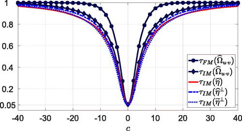
For all tests, power increases symmetrically as c moves away from zero. The traditional D-OLS and FM-OLS based tests have identical local asymptotic power, which is somewhat larger than local asymptotic power of the traditional IM-OLS based test. This is not surprising because the IM-OLS estimator seems to be asymptotically less efficient than the D-OLS and FM-OLS estimators (see Vogelsang and Wagner 2014, Proposition 2). In general, local asymptotic power of the self-normalized tests is similar to but slightly below local asymptotic power of the traditional IM-OLS based test. This is consistent with the findings in the stationary time series literature, where self-normalization is well known to lead to minor power losses (see e.g., Kiefer, Vogelsang, and Bunzel 2000; Shao 2015). Among the self-normalized tests, ${\tau }_{\text{IM}}({\widehat{\eta }}^{\perp })$ performs best, while ${\tau }_{\text{IM}}\left(\widehat{\eta }\right)$ has some performance advantages over ${\tau }_{\text{IM}}({\tilde{\eta }}^{\perp })$ for small to medium deviations from the null hypothesis, but ${\tau }_{\text{IM}}({\tilde{\eta }}^{\perp })$ catches up as c becomes larger.

5.2 Finite Sample Performance

We generate data according to (1) and (2) with m = 2 regressors, that is, $y_t=x_{1t}{\beta }_1+x_{2t}{\beta }_2+u_t,x_{it}=x_{i,t-1}+v_{it}$, i = 1, 2, for $t=1,\dots ,T$, where ${\beta }_1={\beta }_2=1$ and $x_{i0}=0$. The regression errors u_t and the first differences of the stochastic regressors v_it are generated as $$\begin{array}{c}{u}_t={\rho }_1{u}_{t-1}+e_t+\varphi e_{t-1}+{\rho }_2({\nu }_{1t}+{\nu }_{2t}),\hspace{1em}{u}_{-100}=0,\\ v_{it}={\nu }_{it}+0.5{\nu }_{i,t-1},\hspace{1em}{\nu }_{i,-100}=0,\hspace{1em}i=1,2,\end{array}$$for $t=-99,\dots ,0,1,\dots ,T$, where $t=-99,\dots ,0$ serves as a burn-in period to ensure stationarity. The parameters ρ₁ and ρ₂ control the level of error serial correlation and the extent of endogeneity, respectively. For $\varphi \ne 0$ the error process contains a first order moving average component. To construct e_t, ${\nu }_{1t}$, and ${\nu }_{2t}$ we first generate three independent univariate stationary GARCH(1,1) processes ${\xi }_{jt}={\sigma }_{jt}{\epsilon }_{jt}$, j = 1, 2, 3, where ${\sigma }_{jt}^2=a_0+a_1{\xi }_{j,t-1}^2+b_1{\sigma }_{j,t-1}^2$, with ${\xi }_{j,-100}^2=1,{\sigma }_{j,-100}^2=1$, $[{\epsilon }_{1t},{\epsilon }_{2t},{\epsilon }_{3t}]\prime \sim \mathcal{N}(0,I_3)$ iid across t, $a_1,b_1\ge 0$, $a_1+b_1<1$, and $a_0:=1-a_1-b_1$, such that $\mathbb{E}({\xi }_{jt})=0$ and $\mathbb{E}({\xi }_{jt}^2)=\mathbb{E}({\sigma }_{jt}^2)=1$. We then set $[e_t,{\nu }_{1t},{\nu }_{2t}]\prime =L[{\xi }_{1t},{\xi }_{2t},{\xi }_{3t}]\prime$, where L is the lower triangular matrix of the Cholesky decomposition of the matrix with all main diagonal elements equal to one and all off-diagonal elements equal to ρ₃. To impose some weak (cross-sectional) correlation between the three GARCH processes wet set ${\rho }_3=0.2$. Moreover, in line with (Brüggemann, Jentsch, and Trenkler 2016, p. 77), we set $a_1=0.05$ and $b_1=0.94$. The order $1\le q\le \lfloor T^{1/3}\rfloor =:q_{\max }$ of the VAR sieve is chosen as the one that minimizes either the AIC or the BIC computed on the evaluation period $t=q_{\max }+1,\dots ,T$ (Kilian and Lütkepohl 2017, p. 56). We present results for $T\in \{75,100,250\},{\rho }_1={\rho }_2\in \{0,0.3,0.6,0.9\}$ and $\varphi \in \{0,0.3,0.9\}$. In all cases, the number of Monte Carlo and bootstrap replications is 3000 and 499, respectively.

Let us start with analyzing the empirical null rejection probabilities of the traditional and self-normalized Wald-type tests based on asymptotic critical values under the null hypothesis ${\mathrm{H}}_0: {\beta }_1=1, {\beta }_2=1$. The results are benchmarked against the textbook OLS test ${\tau }_{\text{OLS}}({\widehat{\sigma }}_u^2)$, which leads to asymptotically valid inference only in case ${\rho }_1={\rho }_2=\varphi =0$, and against Johansen’s (1995) parametric likelihood ratio (LR) test based on the reduced rank quasi maximum likelihood (QML) estimator in a vector error correction model (VECM) for $X_t:=[y_t,x_{1t},x_{2t}]\prime$ (see Online Appendix C.1 for more details). The order of the VECM is selected by either AIC or BIC. To select the numbers of leads and lags for the construction of the D-OLS estimator, we follow Choi and Kurozumi (2012) and use BIC (which appears to be the most successful criterion in reducing its RMSE) and the upper bounds used in their simulation study (results based on AIC are qualitatively similar). With respect to long-run covariance matrix estimation, we present results for the Bartlett kernel and the quadratic spectral (QS) kernel together with the corresponding data-dependent bandwidth selection rules of Andrews (1991).

Table 1 shows the well known size distortions of the traditional tests whenever ${\rho }_1,{\rho }_2$ is large or T is small. These size distortions can be almost as severe as those of the textbook OLS test. In contrast, the self-normalized tests are considerably less size-distorted than the traditional tests for ${\rho }_1,{\rho }_2<0.9$ and even outperform the LR tests in this case. Because the performance of the IM-OLS estimator is comparable with the performance of the D-OLS and FM-OLS estimators in terms of bias and RMSE (see Table C.4 in Online Appendix C.2), IM-OLS estimation combined with self-normalization serves as a serious alternative to traditional inference in cointegrating regressions. For ${\rho }_1,{\rho }_2=0.9$, however, self-normalization becomes less advantageous, reflecting the poor performance of endogeneity corrections in finite samples when the level of endogeneity and error serial correlation is large. Among the self-normalized tests, the test based on $\widehat{\eta }$ performs best. In particular, adjusting the IM-OLS residuals to remove the correlation between numerator and denominator in the limiting null distribution of ${\tau }_{\text{IM}}(\widehat{\eta })$ has adverse effects on the performance of the test, especially for ${\rho }_1,{\rho }_2=0.9$.

Let us now turn to the performance of the tests based on bootstrap critical values. Table 2 shows that replacing asymptotic critical values with VAR sieve bootstrap critical values (based on AIC) improves the performance of the traditional tests considerably throughout and also reduces the size distortions of the self-normalized tests, especially in case ${\rho }_1,{\rho }_2=0.9$. The bootstrap is thus able to account for finite sample effects of both endogeneity corrections and tuning parameter choices. Results based on BIC are similar, compare Table C.5 in Online Appendix C.2. Performance differences between traditional and self-normalized tests are negligible for small to medium values of ${\rho }_1,{\rho }_2$. For ${\rho }_1,{\rho }_2=0.9$, however, the test based on the D-OLS estimator in combination with the Bartlett kernel often performs best among the traditional tests, while the tests based on $\widehat{\eta }$ and ${\tilde{\eta }}^{\perp }$ perform best among the self-normalized tests and often also perform slightly better than the D-OLS test for sample sizes larger than T = 75 irrespective of the kernel choice. In case T = 75, the D-OLS test based on the Bartlett kernel performs slightly better than the self-normalized test based on $\widehat{\eta }$, which in turn performs slightly better than the D-OLS test based on the QS kernel. Compared to the LR test based on bootstrap critical values (as proposed in Cavaliere, Nielsen, and Rahbek 2015), the traditional and self-normalized tests perform very well as long as ${\rho }_1,{\rho }_2<0.9$, but lead to larger size distortions when ${\rho }_1,{\rho }_2=0.9$ and $T\in \{75,100\}$. However, the reduced rank QML estimator is well known to occasionally produce estimates that are far away from the true parameter values (see, e.g., Brüggemann and Lütkepohl 2005). Thus, it is not surprising that the reduced rank QML estimator has a very large bias and an extremely large RMSE in case ${\rho }_1,{\rho }_2=0.9$ and $T\in \{75,100\}$ compared to the (modified) OLS estimators, see Table C.4 in Online Appendix C.2. This susceptibility to producing outliers can lead to misleading test decisions based on the LR test in applications.

Table 2 also contains the empirical null rejection probabilities of the test statistic ${\tau }_{\text{IM}}(1)$, whose limiting null distribution is given by ${\Omega }_{u·v}{\chi }_2^2$, in conjunction with VAR sieve bootstrap critical values. The test generally performs worse than the traditional and self-normalized tests. This indicates that removing the long-run variance parameter ${\Omega }_{u·v}$ asymptotically—either by direct estimation or by self-normalization—is beneficial in finite samples. Similarly, the traditional and self-normalized tests also outperform the textbook OLS test, with the differences being most pronounced for ${\rho }_1,{\rho }_2=0.9$. Thus, it is advantageous to first account for endogeneity and error serial correlation in the construction of the test statistic before using the VAR sieve bootstrap to construct critical values. We observe similar results also for other choices of the GARCH parameters a₁, b₁, and ρ₃. In particular, the tests based on bootstrap critical values are considerably less size distorted than those based on asymptotic critical values even in case e_t, $v_{1t}$, and $v_{2t}$ are iid standard normally distributed and independent of each other ($a_1=b_1={\rho }_3=0$), compare Tables C.6 and C.7 in Online Appendix C.2.

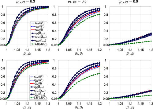
To analyze the properties of the tests under deviations from the null hypothesis, we generate data for ${\beta }_1={\beta }_2\in \left[1,1.2\right]$ using 21 values on a grid with mesh size 0.01. To account for the large performance differences under the null hypothesis, we follow (Cavaliere, Nielsen, and Rahbek 2015, p. 826) and present results based on asymptotic and bootstrap critical values corresponding to the nominal size $\tilde{\alpha }$ that yields empirical null rejection probabilities equal to 5% under the null hypothesis. All size-corrected power curves thus start at 0.05 for ${\beta }_1={\beta }_2=1$. Figure 2 displays illustrative size-corrected power curves of the self-normalized test statistics, the traditional test statistics based on the Bartlett kernel and the LR test statistic based on AIC in combination with asymptotic critical values (top row) and bootstrap critical values (bottom row) for ${\rho }_1,{\rho }_2\in \{0.3,0.6,0.9\}$ in case T = 100 and $\varphi =0.3$. For ${\rho }_1,{\rho }_2=0.3$ the results are in line with the local asymptotic power results analyzed in Section 5.1. The traditional tests based on the FM-OLS and D-OLS estimators are slightly more powerful than the traditional test based on the IM-OLS estimator, which in turn is slightly more powerful than the self-normalized tests. Moreover, the self-normalized tests are as powerful as the LR test. The power loss when replacing asymptotic critical values with bootstrap critical values is negligible for all tests. Increasing ${\rho }_1,{\rho }_2$ reduces power of the tests without altering the relative performance differences with one exception. For ${\rho }_1,{\rho }_2\in \{0.6,0.9\}$ the LR test is considerably less powerful than the traditional and self-normalized tests, irrespective of whether it is based on asymptotic or bootstrap critical values. The difference is even more pronounced for T = 75 but becomes smaller as the sample size increases. The small size distortions of the LR test based on bootstrap critical values under the null hypothesis are thus accompanied by relatively low power under the alternative. With respect to the moving average component in the regression errors, we find that power of the tests is generally largest for $\varphi =0$ and becomes smaller as $\varphi$ increases. The effect is most pronounced for the LR test, especially for $T\in \{75,100\}$. Increasing the sample size is clearly beneficial for all tests, especially in case ${\rho }_1,{\rho }_2=0.9$, compare Figure C.1 in Online Appendix C.2, which shows the results for T = 250. Finally, note that size-corrected power of the self-normalized tests is not necessarily lower than size-corrected power of the traditional tests, see, for example, Figure C.2 in Online Appendix C.2 for ${\rho }_1,{\rho }_2=0.9$, which shows the size-corrected power curves of the traditional tests based on the QS kernel (and of the LR test based on BIC).

Fig. 2 Size-corrected power of the tests for ${\mathrm{H}}_0: {\beta }_1=1, {\beta }_2=1$ at 5% level based on asymptotic critical values (top row) and bootstrap critical values (bottom row) for T = 100 and $\varphi =0.3$. Note: Long-run variance parameters are estimated using the Bartlett kernel and the VAR sieve bootstrap is based on AIC.

6 Empirical Illustration: The Fisher Effect

Many empirical studies suggest that inflation π_t and the short-term nominal interest rate i_t do not cointegrate with the slope of inflation being equal to one. This finding is at odds with the Fisher effect, which is backed by many theoretical models (see, e.g. Westerlund 2008, for a brief description of underlying economic theory). The errors u_t in the Fisher equation $i_t=\alpha +\beta {\pi }_t+u_t,t=1,\dots ,T$, are likely to be highly persistent even in case cointegration between π_t and i_t prevails. Consequently, the Fisher effect might be rejected even if it exists because traditional tests are prone to severe size distortions in this case (see, e.g., Caporale and Pittis 2004; Westerlund 2008). Since self-normalization is less advantageous when the errors are highly persistent, we expect similar results also for the self-normalized tests.

This section illustrates the usefulness of the VAR sieve bootstrap when analyzing the validity of the Fisher effect. We consider the relationship between inflation and the short-term nominal interest rate for 19 OECD countries between 1990Q1 and 2019Q4 (T = 120) using quarterly data (measured at annual rates in percentages) obtained from the OECD databases Economic Outlook and Main Economic Indicators (see Table 3 for details). As a simple persistence measure of the regression errors in the Fisher equation, we regress the OLS residuals on their first lag. The empirical first order autocorrelations lie between 0.88 and 0.95, which indeed indicates highly persistent errors.

Table 3 Realizations of test statistics for ${\mathrm{H}}_0: \beta =1$.

				Traditional tests
	Self-normalized tests			Bartlett kernel			QS kernel
Country	${\tau }_{\text{IM}}({\tilde{\eta }}^{\perp })$	${\tau }_{\text{IM}}({\widehat{\eta }}^{\perp })$	${\tau }_{\text{IM}}(\widehat{\eta })$	${\tau }_{\mathrm{D}}({\widehat{\Omega }}_{u·v})$	${\tau }_{\text{FM}}({\widehat{\Omega }}_{u·v})$	${\tau }_{\text{IM}}({\widehat{\Omega }}_{u·v})$	${\tau }_{\mathrm{D}}({\widehat{\Omega }}_{u·v})$	${\tau }_{\text{FM}}({\widehat{\Omega }}_{u·v})$	${\tau }_{\text{IM}}({\widehat{\Omega }}_{u·v})$
Australia	75.03	553.76	5.22	0.04	1.00	4.66	0.04	0.81	4.10
Austria	$\mathbf{1387}.\mathbf{1}{\mathbf{5}}^{‡}$	2779.14	52.04	0.98	2.76	4.20	0.78	2.30	3.31
Belgium	945.79	3215.69	31.43	0.34	1.22	4.34	0.26	1.26	3.32
Canada	$\mathbf{780}.\mathbf{8}{\mathbf{7}}^{‡}$	1506.10	49.42	0.03	1.21	6.86	0.03	0.84	6.55
Germany	$\mathbf{1543}.\mathbf{3}{\mathbf{1}}^{†}$	$\mathbf{3428}.\mathbf{5}{\mathbf{9}}^{†}$	87.20	3.03	6.77	7.02	2.50	5.56	5.78
Denmark	57.10	188.85	1.68	0.68	4.47	1.38	0.59	4.21	1.20
Spain	221.66	271.51	135.61	4.64	18.63	$\mathbf{16}.\mathbf{5}{\mathbf{1}}^{‡}$	4.31	16.65	$\mathbf{15}.\mathbf{3}{\mathbf{3}}^{‡}$
Finland	396.46	796.37	73.81	0.35	4.08	8.61	0.30	3.40	7.30
France	214.28	1532.73	97.37	2.13	6.30	9.87	1.77	4.97	8.23
United Kingdom	429.67	1324.88	18.83	0.31	1.41	2.03	0.29	1.73	1.90
Ireland	23.67	88.01	2.00	0.04	0.07	0.75	0.03	0.13	0.60
Iceland	15.17	17.59	1.90	1.47	1.63	2.47	1.21	1.33	2.04
Italy	$\mathbf{481}.\mathbf{5}{\mathbf{6}}^{†}$	$\mathbf{736}.\mathbf{2}{\mathbf{9}}^{‡}$	$\mathbf{254}.\mathbf{4}{\mathbf{3}}^{†}$	$\mathbf{14}.\mathbf{6}{\mathbf{4}}^{†}$	$\mathbf{36}.\mathbf{6}{\mathbf{7}}^{†}$	$\mathbf{33}.\mathbf{0}{\mathbf{4}}^{\star }$	$\mathbf{14}.\mathbf{8}{\mathbf{4}}^{†}$	$\mathbf{37}.\mathbf{0}{\mathbf{3}}^{‡}$	$\mathbf{33}.\mathbf{5}{\mathbf{0}}^{\star }$
Netherlands	193.87	671.68	57.02	1.29	0.90	3.75	1.16	0.45	3.37
Norway	370.22	813.18	44.70	0.02	0.48	4.42	0.02	0.25	4.31
New Zealand	159.91	432.83	2.00	0.13	0.67	1.62	0.10	0.57	1.27
Sweden	368.28	1542.48	24.60	0.24	0.93	5.94	0.25	0.64	6.29
United States	206.56	405.61	53.45	1.12	1.10	4.62	0.95	0.92	3.92
South Africa	16.43	30.25	3.35	0.54	0.38	0.60	0.50	0.24	0.56

NOTE: Bold numbers indicate significance at the nominal 10% level based on asymptotic critical values, whereas superscripts $\star ,†$, and $‡$ indicate significance at the nominal 1%, 5%, and 10% level, respectively, based on VAR sieve bootstrap critical values using AIC. The inflation rates and short-term interest rates are available on https://data.oecd.org/price/inflation-cpi.htm and https://data.oecd.org/interest/short-term-interest-rates.htm, respectively (Accessed: March 24, 2022).

To shed some light on the integratedness of the variables, we employ the augmented Dickey-Fuller (ADF) test based on generalized least squares (GLS) demeaning (Elliott, Rothenberg, and Stock 1996) and the KPSS test (Kwiatkowski et al. 1992). All tests are carried out at the nominal 10% level and the bandwidth for long-run variance estimation is always selected with the data-dependent rule of Andrews (1991). Results for the short-term interest rates are unambiguous. The ADF-GLS test (based on AIC with a maximum of five lags) does not reject the null hypothesis of a unit root for any country, whereas the KPSS test (based on the Bartlett kernel) rejects the null hypothesis of stationarity for all countries except Iceland, see Table D.8 in Online Appendix D. The table also presents evidence for a unit root in inflation, but the results are less persuasive. The ADF-GLS test rejects the null hypothesis of a unit root for five countries and the KPSS test decides in favor of stationarity for eleven countries. However, only for Austria, Belgium, and Ireland do both tests decide in favor of stationarity. The results are in line with some parts of the literature questioning an exact unit root in inflation (see, e.g., Jensen 2009). Nevertheless, it is common practice in applications to treat both the interest rate and the inflation rate as integrated processes of order one (see, e.g., Caporale and Pittis 2004, p. 35). To test for cointegration, we employ the group-mean and pooled panel no-cointegration tests developed in Westerlund (2008). The tests are more powerful than single equation no-cointegration tests, especially in the presence of highly persistent errors. Using again the Bartlett kernel for long-run variance estimation, both tests reject the null hypothesis of no-cointegration at the nominal 10% level. The results are robust to different choices for the maximal number of common factors. Moreover, we obtain similar results when the test statistics are constructed under the restriction that β = 1, which already provides some evidence for the validity of the Fisher effect in the individual countries.

We now test the null hypothesis β = 1 for all countries separately using the same test statistics as already analyzed in Section 5.2. Table 3 summarizes the results. For all but three countries, at least one of the nine tests rejects the validity of the Fisher effect when test decisions are based on asymptotic critical values. Moreover, for six countries at least five tests decide against the Fisher effect. Using VAR sieve bootstrap critical values based on AIC (with 499 replications) instead yields different results, with those based on BIC—reported in Table D.9 in Online Appendix D—being similar. For 14 countries none of the tests rejects the validity of the Fisher effect and for additional four countries at most two tests reject the Fisher effect. Hence, after accounting for highly persistent errors, the empirical results support the Fisher effect in OECD countries, which is consistent with many theoretical models. Finally, note that for Italy all bootstrap tests reject the null hypothesis, which serves as strong evidence against the validity of the Fisher effect in this particular country.

7 Summary and Conclusions

To address the severe size distortions of hypotheses tests in cointegrating regressions, this article combines a VAR sieve bootstrap to construct critical values with a self-normalization approach based on the IM-OLS estimator that avoids direct estimation of long-run variance parameters when computing test statistics. To prove bootstrap consistency, we derive a bootstrap invariance principle under mild conditions covering, for example, conditional heteroscedasticity. In addition, the bootstrap invariance principle also allows to prove bootstrap consistency for traditional test statistics based on the D-OLS, FM-OLS, and IM-OLS estimators. Simulation results show that the VAR sieve bootstrap reduces size distortions of hypotheses tests in cointegrating regressions considerably, with two self-normalized test statistics often outperforming the traditional test statistics at the cost of only small power losses. Among the traditional test statistics, the one based on the D-OLS estimator in combination with the Bartlett kernel performs best and turns out to be the closest competitor to the self-normalized test statistics. For the QS kernel, however, the D-OLS based test statistic becomes less competitive. Finally, the empirical illustration demonstrates that replacing asymptotic critical values with VAR sieve bootstrap critical values when analyzing the validity of the Fisher effect in OECD countries leads to alternative conclusions, which are more in line with economic theory.

Possible extensions of the proposed methods to, for example, panels of cointegrating regressions are currently under investigation. Finally, note that a crucial assumption of the article is that the regressors possess an exact unit root, while parts of the literature already allow for nearly integrated regressors (see e.g., Phillips and Magdalinos 2009; Müller and Watson 2013; Hwang and Valdes 2023). However, extending the VAR sieve bootstrap to this setting is not straightforward at all, as constructing bootstrap regressors requires some knowledge of the true local to unity parameters, which are not consistently estimable. Whether the approaches in Phillips, Moon, and Xiao (2001), Phillips (2022), or Hwang and Valdes (2023) help to overcome this limitation will be examined in future research.

Supplementary Materials

The supplementary material contains proofs and additional empirical and simulation results.

Acknowledgments

We are grateful to the editor Atsushi Inoue, an associate editor, and four referees for several insightful and constructive comments that have led to significant changes and improvements of the article. We further thank Katharina Hees, Fabian Knorre, and participants at the Econometrics Colloquium at the University of Konstanz, the IAAE 2021 Annual Conference, the 2021 Asian and North American Summer Meetings of the Econometric Society, and the ${\text{XII}}_t$ Workshop in Time Series Econometrics in Zaragoza for helpful comments. Parts of this research were conducted while Karsten Reichold held a position at the University of Klagenfurt.

Disclosure Statement

The authors have no competing interests to declare.

Data Availability Statement

MATLAB code for empirical applications is available on www.github.com/kreichold/CointSelfNorm

References

- Andrews, D. W. K. (1991), “Heteroskedasticity and Autocorrelation Consistent Covariance Matrix Estimation,” Econometrica, 59, 817–858. DOI: 10.2307/2938229.
- Baillie, R. T., Chung, C. F., and Tieslau, M. A. (1996), “Analysing Inflation by the Fractionally Integrated Arfima–Garch Model,” Journal of Applied Econometrics, 11, 23–40. DOI: 10.1002/(SICI)1099-1255(199601)11:1<23::AID-JAE374>3.0.CO;2-M.
- Benati, L., Lucas Jr., R. E., Nicolini, J. P., and Weber, W. (2021), “International Evidence on Long-Run Money Demand,” Journal of Monetary Economics, 117, 43–63. DOI: 10.1016/j.jmoneco.2020.07.003.
- Bollerslev, T. (1986), “Generalized Autoregressive Conditional Heteroskedasticity,” Journal of Econometrics, 31, 307–327. DOI: 10.1016/0304-4076(86)90063-1.
- Brillinger, D. R. (1981), Time Series: Data Analysis and Theory. San Francisco: Holden-Day, Inc.
- Brüggemann, R., Jentsch, C., and Trenkler, C. (2016), “Inference in VARs with Conditional Heteroskedasticity of Unknown Form,” Journal of Econometrics, 191, 69–85. DOI: 10.1016/j.jeconom.2015.10.004.
- Brüggemann, R., and Lütkepohl, H. (2005), “Practical Problems with Reduced-rank ML Estimators for Cointegration Parameters and a Simple Alternative,” Oxford Bulletin of Economics and Statistics, 67, 673–690. DOI: 10.1111/j.1468-0084.2005.00136.x.
- Bühlmann, P. (1997), “Sieve Bootstrap for Time Series,” Bernoulli, 3, 123–148. DOI: 10.2307/3318584.
- Cai, Y., and Shintani, M. (2006), “On the Alternative Long-Run Variance Ratio Test for a Unit Root,” Econometric Theory, 22, 347–372. DOI: 10.1017/S026646660606018X.
- Caporale, G. M., and Pittis, N. (2004), “Estimator Choice and Fisher’s Paradox: A Monte Carlo Study,” Econometric Reviews, 23, 25–52. DOI: 10.1081/ETC-120028835.
- Cavaliere, G., Nielsen, H. B., and Rahbek, A. (2015), “Bootstrap Testing of Hypotheses on Co-Integration Relations in Vector Autoregressive Models,” Econometrica, 83, 813–831. DOI: 10.3982/ECTA11952.
- Chang, Y., Park, J. Y., and Song, K. (2006), “Bootstrapping Cointegrating Regressions,” Journal of Econometrics, 133, 703–739. DOI: 10.1016/j.jeconom.2005.06.011.
- Choi, I., and Kurozumi, E. (2012), “Model Selection Criteria for the Leads-and-Lags Cointegrating Regression,” Journal of Econometrics, 169, 224–238. DOI: 10.1016/j.jeconom.2012.01.021.
- Dahlhaus, R., Kiss, I. Z., and Neddermeyer, J. C. (2018), “On the Relationship Between the Theory of Cointegration and the Theory of Phase Synchronization,” Statistical Science, 33, 334–357. DOI: 10.1214/18-STS659.
- Elliot, G., Rothenberg, T. J., and Stock, J. H. (1996), “Efficient Tests for an Autoregressive Unit Root,” Econometrica, 64, 813–836. DOI: 10.2307/2171846.
- Engle, R. F. (1982), “Autoregressive Conditional Heteroscedasticity with Estimates of the Variance of United Kingdom Inflation,” Econometrica, 50, 987–1007. DOI: 10.2307/1912773.
- Gonçalves, S., and Kilian, L. (2004), “Bootstrapping Autoregressions with Conditional Heteroskedasticity of Unknown Form,” Journal of Econometrics, 123, 89–120. DOI: 10.1016/j.jeconom.2003.10.030.
- Gonçalves, S., and Kilian, L. (2007), “Asymptotic and Bootstrap Inference for AR(∞) Processes with Conditional Heteroskedasticity,” Econometric Reviews, 26, 609–641.
- Hwang, J., and Sun, Y. (2018), “Simple, Robust, and Accurate F and t Tests in Cointegrated Systems,” Econometric Theory, 34, 949–984. DOI: 10.1017/S026646661700038X.
- Hwang, J., and Valdes, G. (2023), “Low Frequency Cointegrating Regression with Local to Unity Regressors and Unknown Form of Serial Dependence,” Journal of Business & Economic Statistics, Forthcoming. DOI: 10.1080/07350015.2023.2166513.
- Jansson, M. (2002), “Consistent Covariance Matrix Estimation for Linear Processes,” Econometric Theory, 18, 1449–1459. DOI: 10.1017/S0266466602186087.
- Jensen, M. J. (2009), “The Long-Run Fisher Effect: Can It Be Tested?” Journal of Money, Credit and Banking, 41, 221–231. DOI: 10.1111/j.1538-4616.2008.00194.x.
- Jentsch, C., Politis, D. N., and Paparoditis, E. (2015), “Block Bootstrap Theory for Multivariate Integrated and Cointegrated Time Series,” Journal of Time Series Analysis, 36, 416–441. DOI: 10.1111/jtsa.12088.
- Jin, S., Phillips, P. C. B., and Sun, Y. (2006), “A New Approach to Robust Inference in Cointegration,” Economics Letters, 91, 300–306. DOI: 10.1016/j.econlet.2005.12.019.
- Johansen, S. (1995), Likelihood-Based Inference in Cointegrated Vector Auto-Regressive Models, Oxford: Oxford University Press.
- Kiefer, N. M., and Vogelsang, T. J. (2002), “Heteroskedasticity-Autocorrelation Robust Standard Errors Using the Bartlett Kernel Without Truncation,” Econometrica, 70, 2093–2095. DOI: 10.1111/1468-0262.00366.
- Kiefer, N. M., Vogelsang, T. J., and Bunzel, H. (2000), “Simple Robust Testing of Regression Hypotheses,” Econometrica, 68, 695–714. DOI: 10.1111/1468-0262.00128.
- Kilian, L., and Lütkepohl, H. (2017), Structural Vector Autoregressive Analysis, Cambridge: Cambridge University Press.
- Kreiss, J.-P. (1992), “Bootstrap Procedures for AR(∞) Processes,” in Bootstrapping and Related Techniques, Lecture Notes in Economics and Mathematical Systems (Vol. 376), eds. K. H. Jöckel, G. Rothe, and W. Sender, pp. 107–113, Heidelberg: Springer.
- Kuersteiner, G. M. (2001), “Optimal Instrumental Variables Estimation for ARMA Models,” Journal of Econometrics, 104, 359–405. DOI: 10.1016/S0304-4076(01)00088-4.
- Kwiatkowski, D., Phillips, P. C. B., Schmidt, P., and Shin, Y. (1992), “Testing the Null Hypothesis of Stationarity Against the Alternative of a Unit Root,” Journal of Econometrics, 54, 159–178. DOI: 10.1016/0304-4076(92)90104-Y.
- Li, H., and Maddala, G. S. (1997), “Bootstrapping Cointegrating Regressions,” Journal of Econometrics, 80, 297–318. DOI: 10.1016/S0304-4076(97)00043-2.
- Meyer, M., and Kreiss, J.-P. (2015), “On the Vector Autoregressive Sieve Bootstrap,” Journal of Time Series Analysis, 36, 377–397. DOI: 10.1111/jtsa.12090.
- Müller, U. K., and Watson, M. W. (2013), “Low-Frequency Robust Cointegration Testing,” Journal of Econometrics, 174, 66–81. DOI: 10.1016/j.jeconom.2012.09.006.
- Palm, F. C., Smeekes, S., and Urbain, J.-P. (2010), “A Sieve Bootstrap Test for Cointegration in a Conditional Error Correction Model,” Econometric Theory, 26, 647–681. DOI: 10.1017/S0266466609990053.
- Paparoditis, E. (1996), “Bootstrapping Autoregressive and Moving Average Parameter Estimates of Infinite Order Vector Autoregressive Processes,” Journal of Multivariate Analysis, 57, 277–296. DOI: 10.1006/jmva.1996.0034.
- Paparoditis, E., and Politis, D. N. (2003), “Residual-Based Block Bootstrap for Unit Root Testing,” Econometrica, 71, 813–855. DOI: 10.1111/1468-0262.00427.
- Paparoditis, E., and Politis, D. N. (2005), “Bootstrap Hypothesis Testing in Regression Models,” Statistics & Probability Letters, 74, 356–365.
- Park, J. Y. (2002), “An Invariance Principle for Sieve Bootstrap in Time Series,” Econometric Theory, 18, 469–490. DOI: 10.1017/S0266466602182090.
- Phillips, P. C. B. (2014), “Optimal Estimation of Cointegrated Systems With Irrelevant Instruments,” Journal of Econometrics, 178, 210–224. DOI: 10.1016/j.jeconom.2013.08.022.
- Phillips, P. C. B. (2022), “Estimation and Inference with Near Unit Roots,” Econometric Theory, Forthcoming.
- Phillips, P. C. B., and Hansen, B. E. (1990), “Statistical Inference in Instrumental Variables Regression with I(1) Processes,” Review of Economic Studies, 57, 99–125. DOI: 10.2307/2297545.
- Phillips, P. C. B., Leirvik, T., and Storelvmo, T. (2020), “Econometric Estimates of Earth’s Transient Climate Sensitivity,” Journal of Econometrics, 214, 6–32. DOI: 10.1016/j.jeconom.2019.05.002.
- Phillips, P. C. B., and Loretan, M. (1991), “Estimating Long Run Economic Equilibria,” Review of Economic Studies, 58, 407–436. DOI: 10.2307/2298004.
- Phillips, P. C. B., and Magdalinos, T. (2009), “Econometric Inference in the Vicinity of Unity,” Singapore Management University, CoFie Working Paper, 7.
- Phillips, P. C. B., Moon, H. R., and Xiao, Z. (2001), “How to Estimate Autoregressive Roots near Unity,” Econometric Theory, 17, 29–69. DOI: 10.1017/S0266466601171021.
- Politis, D. N., and Romano, J. P. (1994), “The Stationary Bootstrap,” Journal of the American Statistical Association, 89, 1303–1313. DOI: 10.1080/01621459.1994.10476870.
- Psaradakis, Z. (2001), “On Bootstrap Inference in Cointegrating Regressions,” Economics Letters, 72, 1–10. DOI: 10.1016/S0165-1765(01)00410-4.
- Rad, H., Low, R. K. Y., and Faff, R. (2016), “The Profitability of Pairs Trading Strategies: Distance, Cointegration and Copula Methods,” Quantitative Finance, 16, 1541–1558. DOI: 10.1080/14697688.2016.1164337.
- Rho, Y., and Shao, X. (2019), “Bootstrap-Assisted Unit Root Testing With Piecewise Locally Stationary Errors,” Econometric Theory, 35, 142–166. DOI: 10.1017/S0266466618000038.
- Saikkonen, P. (1991), “Asymptotically Efficient Estimation of Cointegrating Regressions,” Econometric Theory, 7, 1–21. DOI: 10.1017/S0266466600004217.
- Shao, X. (2010a), “A Self-Normalization Approach to Confidence Interval Construction in Time Series,” Journal of the Royal Statistical Society, Series B, 72, 343–366. DOI: 10.1111/j.1467-9868.2009.00737.x.
- Shao, X. (2010b), “The Dependent Wild Bootstrap,” Journal of the American Statistical Association, 105, 218–235.
- Shao, X. (2015), “Self-Normalization for Time Series: A Review of Recent Developments,” Journal of the American Statistical Association, 110, 1797–1817.
- Shin, D. W., and Hwang, E. (2013), “Stationary Bootstrapping for Cointegrating Regressions,” Statistics and Probability Letters, 83, 474–480. DOI: 10.1016/j.spl.2012.10.007.
- Stock, J. H., and Watson, M. W. (1993), “A Simple Estimator of Cointegrating Vectors in Higher Order Integrated Systems,” Econometrica, 61, 783–820. DOI: 10.2307/2951763.
- van Giersbergen, N. P. A., and Kiviet, J. F. (2002), “How to Implement the Bootstrap in Static or Stable Dynamic Regression Models: Test Statistic Versus Confidence Region Approach,” Journal of Econometrics, 108, 133–156. DOI: 10.1016/S0304-4076(01)00132-4.
- Vogelsang, T. J., and Wagner, M. (2014), “Integrated Modified OLS Estimation and Fixed-b Inference for Cointegrating Regressions,” Journal of Econometrics, 178, 741–760. DOI: 10.1016/j.jeconom.2013.10.015.
- Wagner, M. (2015), “The Environmental Kuznets Curve, Cointegration and Nonlinearity,” Journal of Applied Econometrics, 30, 948–967. DOI: 10.1002/jae.2421.
- Westerlund, J. (2008), “Panel Cointegration Tests of the Fisher Effect,” Journal of Applied Econometrics, 23, 193–233. DOI: 10.1002/jae.967.
- Wu, W. B., and Min, W. (2005), “On Linear Processes with Dependent Innovations,” Stochastic Processes and their Applications, 115, 939–958. DOI: 10.1016/j.spa.2005.01.001.