Modeling and Forecasting Macroeconomic Downside Risk

Abstract

We model permanent and transitory changes of the predictive density of U.S. GDP growth. A substantial increase in downside risk to U.S. economic growth emerges over the last 30 years, associated with the long-run growth slowdown started in the early 2000s. Conditional skewness moves procyclically, implying negatively skewed predictive densities ahead and during recessions, often anticipated by deteriorating financial conditions. Conversely, positively skewed distributions characterize expansions. The modeling framework ensures robustness to tail events, allows for both dense or sparse predictor designs, and delivers competitive out-of-sample (point, density and tail) forecasts, improving upon standard benchmarks.

Keywords:

• Business cycle
• Downside risk
• Financial conditions
• Score driven
• Skewness

1 Introduction

The Global Financial Crisis and the subsequent recession left policymakers with several new challenges to face. In a world of persistently sluggish growth, subject to infrequent but deep recessions, the idea of central bankers as “risk managers” gained renewed popularity (see, e.g., Cecchetti 2008). In this environment, policy makers pursuing a “plan for the worst, hope for the best” approach rely on downside risk measures to assess the distribution of risk around modal forecasts. Yet, gauging the degree of asymmetry of business cycle fluctuations remains a challenging task, and even more so it is to reliably assess the time variation of downside risk. In addition, sound economic policy should consider the evolution of secular macroeconomic trends in pursuing the long-run goals of price stability and sustainable economic growth. In this article, we introduce a generalized, comprehensive framework fit to provide policy guidance on the developments of downside risks, tracking permanent and transitory changes in the conditional distribution of GDP growth.

We provide novel evidence in support of time-varying conditional asymmetry of GDP growth’s distribution. Despite unconditional asymmetry remains unsupported by the data, conditional skewness, and thus downside risk to economic growth, exhibits significant time variation. Motivated by this evidence, we introduce a novel, flexible methodology that allows us to track and predict time-varying skewed Student-t (Skew-t) conditional densities, where the time variation of the location, scale, and asymmetry parameters is driven by the score of the predictive likelihood function (Creal, Koopman, and Lucas 2013; Harvey 2013), as well as by a set of observed predictors. The latter allow us to explore to what extent downside risk to economic growth reflects imbalances arising in financial markets (Adrian, Boyarchenko, and Giannone 2019). When assessed based on its out-of-sample performance, our model delivers well calibrated predictive densities, improving upon competitive benchmarks in terms of point, density and tail forecasts, as well as leading to timely predictions of the odds of forthcoming recessions.

We provide novel evidence on the permanent and transitory evolution of macroeconomic downside risk. Over the last 30 years, skewness has decreased steadily, implying a higher exposure to downside risk, which partially accounts for the slowdown in long-run growth observed since the early 2000s. Similarly, we document that the fall in macroeconomic volatility since the mid-1980s, the so called Great Moderation, reflects a significant reduction of upside volatility, with downside volatility remaining stable over the same period. Over the short-term, conditional skewness varies procyclically, so that at the onset of downturns, business cycle exhibits significant negative skewness, while expansions are characterized by positively skewed distributions. Therefore, the well-documented counter-cyclicality of GDP growth’s volatility largely reflects increasing downside volatility during recessions. The extreme realizations of the pandemic quarters are captured through movements in volatility and skewness, allowing the model to remain remarkably stable and suggesting that such outcomes were, to some extent, tail events.

We show that the inclusion of the four subcomponents of the National Financial Conditions Index (NFCI, Brave and Butters 2012), capturing risk, credit, leverage and nonfinancial leverage developments, improves the out-of-sample forecasting accuracy of our model, in particular during recessions. Financial deepening during expansions is associated with positive GDP growth’s skewness, whereas tightening of financial conditions, especially the build-up of household debt, consistently predicts downside risk episodes. Although aggregate measures succeed in summarizing a large amount of data, concerns that information relevant for assessing risk can remain undetected persist. To this end, we investigate whether different patterns of sparsity can arise in predicting different features of the conditional distribution of GDP growth. We follow the “shrink-then-sparsify” approach of Hahn and Carvalho (2015), where sparsity is achieved by means of the Signal Adaptive Variable Selector (SAVS) of Ray and Bhattacharya (2018).¹ The build-up of financial institutions’ and households’ leverage, as well as credit conditions, receive the least shrinkage over the full sample. We also show that indicators of the balance sheet of the intermediary sector (Adrian and Shin 2008), as well as growing imbalances in the housing market (see, e.g., Gertler and Gilchrist 2018) were important to timely assess increasing downside risks ahead and during the financial crisis. Processing the signal from a large panel of financial predictors leads to improvements in short-term predictions, especially during 2020.

Our results highlight the importance of accounting for asymmetric business cycle fluctuations. These can emerge through nonlinearities in the transmission of Gaussian shocks (see Fernández-Villaverde and Guerrón-Quintana 2020), or reflect conditionally skewed shocks hitting the economy (as in Bekaert and Engstrom 2017; Salgado, Guvenen, and Bloom 2019). Our results emphasize (i) the necessity to distinguish between “good” and “bad” uncertainty, which can potentially impact economic activity in opposite directions (Segal, Shaliastovich, and Yaron 2015), (ii) the need to account for the nonlinear relationship between financial conditions and credit availability, and the distribution of GDP growth for policy monitoring and stabilization policy design (Adrian et al. 2020), and (iii) that the fall in trend-skewness of economic growth, and the associated increase of downside risk over the last three decades, emerge as salient features of the data that need to be accounted for by theoretical macroeconomic models (see, e.g., Jensen et al. 2020).

1.1 Related Literature

This article builds on the growing literature exploring the asymmetry characterizing business cycle fluctuations, and the relationship between real economic activity and financial conditions. Giglio, Kelly, and Pruitt (2016) and Adrian, Boyarchenko, and Giannone (2019) uncover a significant negative correlation between financial conditions and the lower quantiles of the conditional distribution of future economic growth, by means of quantile regressions. We introduce a novel approach based on the modeling of the parameters of a Skew-t distribution. Our approach is based on a rich, yet parsimonious structure, and directly provides conditional densities. Our model captures persistence in the skewness of the distribution of GDP growth, consistently with the term structure of growth-at-risk displaying stronger asymmetry for the short- than for the medium-run (Adrian et al. 2022), and with the Survey of Professional Forecasters’ short-term density predictions (Ganics, Rossi, and Sekhposyan 2020). Differently to other contributions (see, e.g., Adrian, Boyarchenko, and Giannone 2019; Plagborg-Møller et al. 2020), we model permanent and transitory changes of the distribution of GDP growth. This is essential to recover well-known stylized facts, such as the Great Moderation (McConnell and Perez-Quiros 2000; Stock and Watson 2002) and the fall in long-run growth (Antolin-Diaz, Drechsel, and Petrella 2017; Eo and Morley 2022), and to uncover negative, decreasing business cycle skewness over the last 30 years.

A number of recent contributions have called into question the presence of asymmetry in business cycle fluctuations (see, e.g., Carriero, Clark, and Marcellino Forthcoming). Our approach allows for, but does not impose, skewness in the conditional distribution. Yet, we document significant variation in the asymmetry of GDP growth. Allowing for time-varying asymmetry leads to substantial gains in out-of-sample forecasts and downside risk predictions over standard volatility models, whose competitiveness has recently been highlighted by Clark and Ravazzolo (2015) and Brownlees and Souza (2021).

Existing models for conditional skewness rely on ad hoc laws of motion for the time-varying parameters, and the asymmetry is updated as a function of higher-order powers of the residuals (Hansen 1994; Harvey and Siddique 1999). We, instead, rely on the score-driven framework put forward by Creal, Koopman, and Lucas (2013) and Harvey (2013), which readily accommodates parameters’ time variation under different distributional assumptions (Koopman, Lucas, and Scharth 2016). Hence, parameters update according to (highly) nonlinear functions of past prediction errors, depending, among other, on the shape of the conditional distribution. Thus, not only the updating mechanism adapts to the local properties of the data, but it is also robust to the presence of extreme realizations, contrary to updates based on higher-order powers of the residuals. Within the score-driven setting, to the best of our knowledge, we are the first to rely on Bayesian estimation methods. This allows us to jointly tackle parameters’ proliferation and overfitting, as well as incorporate estimation uncertainty when assessing the predictions of the model.

1.2 Structure

The remainder of the article is organized as follows. Section 2 provides evidence of time-varying business cycle asymmetry. Section 3 presents the model, the estimation approach and the forecasting procedure. In Section 4 we discuss the features of the conditional distribution of GDP growth, and their relation to financial predictors. Section 5 reports the out-of-sample forecast and downside risk prediction evaluation. In Section 6 we investigate the predictive ability of the large set of financial indicators. Section 7 concludes.

2 Motivating Evidence

Assessing the degree of skewness of GDP growth is notoriously challenging. Over the 1973–2020 (1973–2019) sample, unconditional skewness is–2.58 (–0.42), but one cannot reject the null of symmetry using the Bai and Ng (2005) test. However, the absence of skewness in the unconditional distribution, does not imply conditional distributions being symmetric as well (Carriero, Clark, and Marcellino Forthcoming). The low precision of skewness estimates can potentially reflect the dynamic nature of the asymmetry of economic fluctuations.²

Harvey (2013, sec. 2.5) highlights that the Lagrange Multiplier principle can be employed to construct appropriate test statistics for the time variation of parameters (see Appendix A). Starting from the assumption that GDP growth follows an AR(2) process with Skew-t innovations, with a shape parameter pinning down the degree of asymmetry, we test for the time variation of this parameter considering both the case of constant volatility and the more realistic case of time-varying volatility. Table 1 reports the statistics for the Portmanteau (Q), Ljung-Box ($Q^{*}$), and Nyblom (N) tests. The null hypothesis of a constant shape parameter is strongly rejected against the alternative of time variation; the rejection of the Nyblom test suggests that the parameter is likely to be highly persistent.

Table 1 Score-based tests for time variation.

	Time-varying			Time-varying
	Location			Location & scale
	Q	$Q^{*}$	N	Q	$Q^{*}$	N
Scale^2	7.187***	7.296***	0.979***
Shape	8.497***	8.626***	0.603**	22.608***	22.951***	1.053***

NOTE: Q is the portmanteau test, $Q^{*}$ is the Ljung-Box extension (both with automatic lag selection) and N corresponds to the Nyblom test. Q and $Q^{*}$ are distributed as a ${\chi }_1^2$, while N is distributed as a Cramer von-Mises distribution with 1 degree of freedom. $*p<10\%,**p<5\%,***p<1\%$.

Starting from this novel evidence, we introduce a modeling framework that allows us to track the time-varying asymmetry in the conditional distribution of GDP growth.

3 A Time-Varying Skew-t Model for GDP Growth

Let y_t denote the annualized quarter-on-quarter GDP growth at time t. We assume its conditional distribution can be characterized by a Skew-t (Arellano-Valle, Gómez, and Quintana 2005; Gómez, Torres, and Bolfarine 2007), with time-varying location μ_t , scale σ_t , and shape ${\varrho }_t$ parameters: (1) $$y_t={\mu }_t+{\epsilon }_t,\mathrm{\hspace{1em}}\mathrm{\hspace{1em}}{\epsilon }_t\sim Sk{t}_{\nu }(0,{\sigma }_t,{\varrho }_t),\hspace{1em}t=1,\dots ,T,$$(1) with constant degrees of freedom $\nu >3,{\sigma }_t>0$, and ${\varrho }_t\in (-1,1)$. The shape parameter fully characterizes the asymmetry of the distribution, with $\frac{1+{\varrho }_t}{1-{\varrho }_t}$ defining the ratio of the probability mass on the right, over the probability mass on the left of the mode, μ_t . Therefore, negative (positive) values of ${\varrho }_t$ imply negatively (positively) skewed distributions. The conditional log-likelihood function of the observation is (2) $$\begin{array}{c}{\mathcal{l}}_t=\hspace{0.17em}\log \hspace{0.17em}p(y_t|\theta ,{\mathcal{Y}}^{t-1})=\hspace{0.17em}\log \hspace{0.17em}\mathcal{C}(\eta )-\frac{1}{2}\log \hspace{0.17em}{\sigma }_t^2\\ \hspace{1em}-\frac{1+\eta }{2\eta }\{\begin{array}{c}\hspace{0.17em}\log \hspace{0.17em}\left[1+\frac{\eta {\epsilon }_t^2}{{(1+{\varrho }_t)}^2{\sigma }_t^2}\right],\hspace{1em}{\epsilon }_t\ge 0\hfill \\ \hspace{0.17em}\log \hspace{0.17em}\left[1+\frac{\eta {\epsilon }_t^2}{{(1-{\varrho }_t)}^2{\sigma }_t^2}\right],\hspace{1em}{\epsilon }_t<0\hfill \end{array},\end{array}$$(2) with $\eta =\frac{1}{\nu },\mathcal{C}(\eta )=\frac{\sqrt{\eta }\Gamma \left(\frac{1+\eta }{2\eta }\right)}{\sqrt{\pi }\Gamma \left(\frac{1}{2\eta }\right)}$, and $\Gamma (·)$ is the Gamma function. The vector $\theta \in \Theta$ is the vector of static parameters of the model, and ${\mathcal{Y}}^{t-1}$ is the information set up to time $t-1$. For ${\varrho }_t=0$ we have the symmetric Student-t distribution, for $\eta \to 0$ we retrieve the epsilon-Skew-Gaussian distribution of Mudholkar and Hutson (2000), whereas the distribution collapses to a Gaussian density when both conditions hold. Thus, we allow for, but do not impose, skewness in the conditional distribution of GDP growth. We model the time variation of the parameters within the score driven framework of Creal, Koopman, and Lucas (2013) and Harvey (2013). In order to ensure the scale σ_t to be positive and the shape ${\varrho }_t\in (-1,1)$, we model ${\gamma }_t=\hspace{0.17em}\log \hspace{0.17em}({\sigma }_t)$ and ${\delta }_t=\text{arctanh}({\varrho }_t)$.³ Therefore, the vector of time-varying parameters is $f_t=[{\mu }_t,{\gamma }_t,{\delta }_t]\prime$ and takes values in the domain ${\mathcal{F}}_{\theta }$. The updating mechanism follows:⁴ (3) $$f_{t+1}=A{s}_t+B{f}_t+C{X}_t,\hspace{1em}t=1,\dots ,T,$$(3) where A collects the parameters governing the learning rates from the scaled score, s_t , which we define as an appropriate transformation of the prediction error, B contains autoregressive parameters, and C collects loadings on a potential set of covariates X_t . Specifically, $s_t={\stackrel{.}{\mathcal{S}}}_t^{-1}{\dot{\nabla }}_t$ is the scaled score, with ${\dot{\nabla }}_t=\frac{\partial {\mathcal{l}}_t}{\partial f_t}=J_t^{\prime }{\nabla }_t$, where ${\nabla }_t=\left[\frac{\partial {\mathcal{l}}_t}{\partial {\mu }_t},\frac{\partial {\mathcal{l}}_t}{\partial {\sigma }_t^2},\frac{\partial {\mathcal{l}}_t}{\partial {\varrho }_t}\right]\prime$ is the gradient of the log-likelihood function with respect to the location, squared scale and shape parameter, and J_t is the Jacobian matrix associated to the nonlinear transformation of the time-varying parameters. ${\stackrel{.}{\mathcal{S}}}_t$ is a scaling matrix, set as a smoothed version of the diagonal of the Information matrix: ${\stackrel{.}{\mathcal{S}}}_t=(1-\chi ){\stackrel{.}{\mathcal{S}}}_{t-1}+\chi {(J_t^{\prime }\text{diag}({\mathcal{I}}_{\mathit{t}})J_t)}^{\frac{1}{2}}$, where ${\mathcal{I}}_{\mathit{t}}=\mathbb{E}[{\nabla }_t{\nabla }_t^{\prime }]$, and $0<\chi <1$ is estimated jointly with θ. Hence, each element of the score vector has (approximately) unit variance, and is proportional to the respective gradient.⁵ Smoothing ${\stackrel{.}{\mathcal{S}}}_t$ makes it less sensitive to a single observation, avoids instabilities when $|{\varrho }_t|\to 1$, and renders the filtering process more robust (see, e.g., Creal, Koopman, and Lucas 2013).

The resulting model belongs to the class of observation-driven models, for which the trajectories of the time-varying parameters are perfectly predictable one-step-ahead given past information, and the log-likelihood function is available in closed form (Cox 1981). The following Proposition provides the closed form expressions for the gradient and the associated Information matrix.

Proposition 1.

Given the specification in (1) and the likelihood in (2), the elements of the gradient ${\nabla }_t$, with respect to the location, squared scale and shape parameters, are (4) $$\begin{array}{c}{\nabla }_{\mu ,t}=\frac{1}{{\sigma }_t}{w}_t{\zeta }_t,\hspace{1em}{\nabla }_{{\sigma }^2,t}=\frac{1}{2{\sigma }_t^2}(w_t{\zeta }_t^2-1),\\ \hspace{1em}{\nabla }_{\varrho ,t}=\frac{\mathit{sgn}({\epsilon }_t)}{(1+\mathit{sgn}({\epsilon }_t){\varrho }_t)}{w}_t{\zeta }_t^2,\end{array}$$(4) where $w_t=\frac{(1+\eta )}{{(1+\mathit{sgn}({\epsilon }_t){\varrho }_t)}^2+\eta {\zeta }_t^2}$ and ${\zeta }_t=\frac{{\epsilon }_t}{{\sigma }_t}$ denotes the standardized prediction error, and $\mathit{sgn}(·)$ is the sign function. The associated Information matrix reads: (5) $${\mathcal{I}}_{\mathit{t}}=\mathbb{E}[{\nabla }_t\nabla {\prime }_t]=\left[\begin{array}{ccc}\frac{\left(1+\eta \right)}{{\sigma }_t^2(1-{\varrho }_t^2)\left(1+3\eta \right)}& 0& \frac{4\mathcal{C}(1+\eta )}{{\sigma }_t(1-{\varrho }_t^2)(1+3\eta )}\\ 0& \frac{1}{2(1+3\eta ){\sigma }_t^4}& 0\\ \frac{4\mathcal{C}(1+\eta )}{{\sigma }_t(1-{\varrho }_t^2)(1+3\eta )}& 0& \frac{3(1+\eta )}{(1-{\varrho }_t^2)(1+3\eta )}\end{array}\right]\mathrm{}.$$(5)

Defining $f_t={[{\mu }_t,{\gamma }_t,{\delta }_t]}^{\prime }$, where ${\gamma }_t=\hspace{0.17em}\log \hspace{0.17em}({\sigma }_t)$ and ${\delta }_t=\text{arctanh}({\varrho }_t)$, the Jacobian matrix, $J_t=\frac{\partial [{\mu }_t,{\sigma }_t^2,{\varrho }_t]}{\partial [{\mu }_t,{\gamma }_t,{\delta }_t]\prime }$, is diagonal with elements $\left[1,2{\sigma }_t^2,1-{\varrho }_t^2\right]$.

Proof.

See Appendix B. □

Proposition 1 highlights the central role of re-weighting the standardized prediction error for the updating of the time-varying parameters. Weights, w_t , penalize extreme innovations depending on the thickness of the tails, as well as the estimated volatility and asymmetry as of time t. The top left panel of Figure 1 displays the weights associated with the prediction error, for alternative model parameterizations. In a Gaussian setting (black line) weights are constant and equal to unity, implying no discounting. When the asymmetry parameter is zero (red line), the weights display the classic outlier-discounting typical of the Student-t distributions. When the distribution is positively (negatively) skewed, that is, for ${\varrho }_t>0$ (${\varrho }_t<0$), negative (positive) prediction errors, being less likely in expectation, command a larger update of the parameters. This asymmetric treatment of ζ_t is more pronounced as skewness grows larger (i.e., $|{\varrho }_t|\to 1$).

Fig. 1 Prediction error and parameters’ updating.

NOTE: The figures plot the weighting scheme implied by w_t , and the scaled scores, for different values of the standardized prediction error ${\zeta }_t=\frac{{\epsilon }_t}{{\sigma }_t}$. We consider the Gaussian case (black), the symmetric t₅ (red), and positively (blue) and negatively (green) Skt₅.

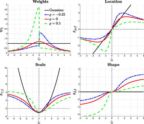
To illustrate how the standardized prediction errors translate into updates for the time-varying parameters, Figure 1 plots the scaled scores for χ = 1 (i.e., no smoothing), (6) $$\begin{array}{c}{s}_{\mu ,t}=\sqrt{\frac{\left(1+3\eta \right)(1+{\varrho }_t^2)}{\left(1+\eta \right)}}{w}_t{\zeta }_t,s_{\gamma ,t}=\sqrt{\frac{(1+3\eta )}{2}}(w_t{\zeta }_t^2-1),\\ \hspace{1em}{s}_{\delta ,t}=\mathit{sgn}({\epsilon }_t)\sqrt{\frac{(1+3\eta )(1-\mathit{sgn}({\epsilon }_t){\varrho }_t)}{3(1+\eta )(1+\mathit{sgn}({\epsilon }_t){\varrho }_t)}}{w}_t{\zeta }_t^2\end{array}$$(6) against the standardized innovations. The location updates in the direction of the prediction error. When the distribution is Gaussian, the update is linear in the prediction error as in traditional state-space models. Heavy tails introduce an outlier discounting implying the typical S-shaped influence function (see, e.g., Harvey and Luati 2014; Delle Monache and Petrella 2017), which in our case adapts to the asymmetry of the conditional distribution. The shape updates in the same direction of the prediction error, such that for negative innovations the distribution becomes more left skewed. On the contrary, updates of the scale only depend on the magnitude of the prediction errors: σ_t increases for $w_t{\zeta }_t^2>1$, and decreases otherwise. Whereas the scores for the location and shape parameters are positively correlated ($\text{corr}(s_{\mu ,t},s_{\delta ,t})=\frac{4\mathcal{C}}{\sqrt{3}}$), updates of σ_t are (unconditionally) uncorrelated with revisions of the other parameter (see the Information matrix in (5)). Yet, at the onset of recessions, when prediction errors are large and negative, updates of the scale and shape parameters negatively comove, such that dispersion increases and negative skewness deepens.

The updating mechanism associated with the scores in (6) depends on the parameters conditional at time t. For a given prediction error, the magnitude of the updates is smaller when large errors are expected, that is when the scale is large. The asymmetry of the distribution plays a key role in mapping the prediction error into parameters’ updates. When the distribution is left skewed, a positive (negative) prediction error leads to stronger (weaker) updates, while the opposite is true for positive skew. This property allows the model to timely detect shifts in the skewness of GDP growth around business cycle turning points. For instance, whenever a large, negative innovation arrives at the peak of the cycle, the model promptly updates ${\varrho }_t$, often resulting in a change of sing of the conditional skewness. In addition, the updating mechanism is robust to the presence of outliers, as parameters’ updates are inelastic to extreme standardized innovations. Hence, the model remains well-behaved despite abnormal prediction errors, as observed in 2020.

Existing models allowing for asymmetric t innovations with time-varying conditional skewness feature updating mechanisms based on simple higher-order powers of the prediction errors (see, e.g., Hansen 1994; Harvey and Siddique 1999). These updating present two main drawbacks. First, the mapping between innovations and time-varying parameters does not depend on the local properties of conditional distributions. For instance, these specifications do not account for the higher probability of negative prediction errors when the conditional distribution is negatively skewed. Second, higher-order powers of the innovations make the time-varying parameters inherently sensitive to large prediction errors, and can thus become unstable in the presence of outliers. Both of those issues are taken care of by our score-driven updates.

Blasques, Koopman, and Lucas (2015) show that, in line with the logic of the Gauss-Newton method for optimization, score-driven updates in a setting with a single time-varying parameter reduce the local Kullback-Leibler divergence between the true and the model-implied conditional density, provided the learning rate is positive and sufficiently small. We opt for a diagonal scaling matrix for the score, such that the updates in our model mimic a Quasi-Newton multivariate optimization methods.⁶ Then, for small and positive learning rates, updates are expected to locally improve the log-likelihood, in that, after an update, the fit would improve if the next observation was much like the current.⁷ In Appendix E we show that this set up, in a simulation setting, achieves lower KL divergence values and presents better updating properties compared to the alternative specifications of Hansen (1994) and Harvey and Siddique (1999).

3.1 Permanent and Transitory Components

When modeling the conditional distribution of GDP growth, it is important to allow for permanent and transitory movements of the moments. Several papers have documented significant changes in the long-run mean of GDP growth (see, e.g., Antolin-Diaz, Drechsel, and Petrella 2017; Doz, Ferrara, and Pionnier 2020; Eo and Morley 2022), as well as shifts in the volatility (McConnell and Perez-Quiros 2000; Stock and Watson 2002), and the skewness of the distribution (Jensen et al. 2020) since the late 1980s. At the same time, Jurado, Ludvigson, and Ng (2015) show that GDP growth volatility is countercyclical, while Giglio, Kelly, and Pruitt (2016) and Adrian, Boyarchenko, and Giannone (2019) argue that business cycle skewness falls sharply during recessions.

To account for these features, we postulate a two-component specification for the time-varying parameters, in the spirit of Engle and Lee (1999). We posit a random walk updating for the permanent components, where these are able to track both smooth variations and sudden breaks of the parameters. Moreover, we allow a set of predictors, X_t , to have a transitory impact on the parameters of the distribution. Introducing a permanent and transitory decomposition of the time-varying parameters implies a linear transformation of the original parameters, hence, leaving the scaled score unchanged.

The location is linear in the permanent and transitory components: ${\mu }_t={\overline{\mu }}_t+{\tilde{\mu }}_t$, with (7) $$\begin{array}{c}{\overline{\mu }}_{t+1}={\overline{\mu }}_t+{\varsigma }_{\mu }{s}_{\mu ,t},\hspace{1em}\text{and }\\ \hspace{1em}{\tilde{\mu }}_{t+1}={\varphi }_{\mu ,1}{\tilde{\mu }}_t+{\varphi }_{\mu ,2}{\tilde{\mu }}_{t-1}+{\beta }_{\mu }^{\prime }{X}_t+{\kappa }_{\mu }{s}_{\mu ,t},\end{array}$$(7) where the AR(2) specification for ${\tilde{\mu }}_{t+1}$ is able to recover the characteristic hump shaped impulse response of the data (Chauvet and Potter 2013). Following Engle and Rangel (2008), we assume a multiplicative specification for σ_t ; hence, $\hspace{0.17em}\log \hspace{0.17em}({\sigma }_t)={\gamma }_t={\overline{\gamma }}_t+{\tilde{\gamma }}_t$, and (8) $${\overline{\gamma }}_{t+1}={\overline{\gamma }}_t+{\varsigma }_{\gamma }{s}_{\gamma ,t},\hspace{1em}\text{and }\hspace{1em}{\tilde{\gamma }}_{t+1}={\varphi }_{\gamma }{\tilde{\gamma }}_t+{\beta }_{\gamma }^{\prime }{X}_t+{\kappa }_{\gamma }{s}_{\gamma ,t}.$$(8)

Similarly, we set ${\delta }_t={\overline{\delta }}_t+{\tilde{\delta }}_t$ for the transformed shape parameter, ${\delta }_t=\text{arctanh}({\varrho }_t)$, with (9) $${\overline{\delta }}_{t+1}={\overline{\delta }}_t+{\varsigma }_{\delta }{s}_{\delta ,t},\hspace{1em}\text{and }\hspace{1em}{\tilde{\delta }}_{t+1}={\varphi }_{\delta }{\tilde{\delta }}_t+{\beta }_{\delta }^{\prime }{X}_t+{\kappa }_{\delta }{s}_{\delta ,t}.$$(9)

Therefore, the resulting vector of time-varying parameters becomes $f_t=({\overline{\mu }}_t,{\tilde{\mu }}_t,{\overline{\gamma }}_t,{\tilde{\gamma }}_t,{\overline{\delta }}_t,{\tilde{\delta }}_t)\prime$, with the law of motion being a restricted specification of (3) (see Appendix B).

Plagborg-Møller et al. (2020) consider a time-varying Skew-t specification for GDP growth and specify the time-varying parameters (location, log-scale and shape) as linear functions of a set of predictors. In this case—which remains nested within our setting—the sole source of parameters’ variation stems from the dynamics of the predictors. This modeling choice generates substantial variability in the underlying parameters, and thus uncertainty around the estimates. In contrast, our specification allows for both secular and transitory shifts in the parameters, where the autoregressive structure of the transitory components makes them functions of discounted values of all past predictors and past scores (i.e., nonlinear functions of past data). As a result, the time-varying parameters we estimate are smoother and less affected by the noise in the data.⁸

3.2 Estimation

A feature of observation-driven models is the straightforward computation of the likelihood function (Creal, Koopman, and Lucas 2013; Harvey 2013). However, the optimization and computation of confidence intervals remain challenging, in particular when these models feature rich parameterizations. Bayesian estimators, which rely on Markov chain Monte Carlo (MCMC) methods, represent a tractable and theoretically attractive alternative to the extremum-based estimation and inference (see, e.g., Vrontos, Dellaportas, and Politis 2000). In fact, under appropriate regularity conditions, asymptotic results guarantee that simulations from a Markov chain provide, after some burn-in period and sufficient iterations, samples from the posterior distribution of interest (for details, see Smith and Roberts 1993; Besag et al. 1995).⁹ In addition, relying on MCMC provides a simple approach to compute any posterior summary of interest as a function of the parameters, for example credible intervals for the time-varying moments of the distribution. Lastly, within a Bayesian setting we can easily incorporate parameter uncertainty when producing forecasts, which turns out to be critical for enhancing the reliability of density forecasts, in particular for downside risk predictions.

Taking a Bayesian perspective also allows us to impose realistic priors on the static parameters, $\pi (\theta )$. We choose priors that in small samples alleviate the problem of parameter proliferation and overfitting, while for large samples the estimation is eventually dominated by the information in the data. Our choices encode the view that transitory components are smooth and stationary, while permanent components capture slow-moving trends. We assume inverse gamma priors for the score loadings, as we expect these parameters to be positive. Moreover, we expect the learning rate in the transitory components (κ) to be larger than those of the permanent components (Ϛ), such that on impact the former react more to innovations with respect to the latter. This is reflected into a tighter scale for the prior distribution of Ϛ.¹⁰ We set Minnesota-type priors for the AR coefficients ($\varphi$) of the transitory components, centered around high persistence values. For the location’s AR parameters, we also introduce a prior on the sum of coefficients. For the loadings on the explanatory variables (β) we assume Normal priors centered around zero, with tight scales to avoid overfitting, in the fashion of L₂ regularization. We assume an inverse gamma prior for η. Lastly, we also estimate the initial values of the permanent components assuming independent Gaussian priors centered around historical average values for the three parameters, and with reasonably small variance.

Blasques et al. (2022) underline the importance of filter invertibility for the consistency of the maximum likelihood estimation, and provide the following sufficient condition for invertibility: $\mathbb{E}\hspace{0.17em}\log \hspace{0.17em}\left\{su{p}_{f\in {\mathcal{F}}_{\theta }}\left|B+A\frac{\partial s(f,y_t,\theta )}{\partial f{\prime }_t}\right|\right\}<0$, (see also Blasques et al. 2018).¹¹ Ensuring the invertibility of nonlinear time series processes with more than one time-varying parameter is usually a major challenge, and so is finding the compact set for which the condition is met for our specification. Nonetheless, we can effectively restrict the estimated parameters to verify the empirical version of the invertibility condition, $\frac{1}{T}{\sum }_{t=1}^T\hspace{0.17em}\log \hspace{0.17em}\left|B+A\frac{\partial s(f,y_t,\theta )}{\partial f{\prime }_t}\right|<0$, by means of a rejection step in our sampler.¹²

Draws from the posteriors are generated using an Adaptive Random-Walk Metropolis-Hastings algorithm (Haario, Saksman, and Tamminen 1999), with the chain initialized at the Maximum likelihood estimates. For each draw θ^j , we compute the time-varying parameters ${\left\{f_t\right|{\theta }^j\}}_{t=0}^T$, and the log-likelihood $\mathcal{l}(y|{\theta }^j)={\sum }_{t=1}^T{\mathcal{l}}_t$. We accept the current draw with probability $p=\min \{1,\hspace{0.17em}\exp \hspace{0.17em}(\pi ({\theta }^j|y)-\pi (\theta \prime |y))\}$, where $\pi ({\theta }^j|y)\propto \pi ({\theta }^j)\mathcal{l}(y|{\theta }^j)$ is the posterior distribution of θ^j ; when accepted, we set $\theta \prime ={\theta }^j.$ Credible sets for both static and time-varying parameters are obtained from the empirical distribution functions arising from the resampling. Appendix D provides an extensive description of the sampling algorithm, details on the exact prior specification for the parameters and convergence diagnostics. Moreover, we show that the informative priors that we have chosen remain agnostic with respect to all the stylized facts documented in Section 4 of the article.

3.2.1 Monte Carlo Exercise

Appendix E investigates the small sample properties of the model through a Monte Carlo analysis. The model successfully tracks parameters’ time variation from different data generating processes. When the distribution is symmetric throughout the entire sample, the model estimates a null shape parameter, with limited variability over time. In particular, the model does not confound any correlation between the time variation of the location and the scale (known to generate unconditional skewness) for the presence of conditional asymmetry. We also simulate a one-time break in the shape parameter: the model correctly captures the break in the asymmetry, and the two-component specification properly disentangles long- and short-lived fluctuations, so that the break is tracked by the permanent component whereas the transitory component features low variability.

3.3 Forecasts

For any draw of the parameters, θ, the filter in (3) provides the one-step ahead prediction of the parameters, $f_{T+1}$. Therefore, the associated forecast is $p(y_{T+1})=\int p(y_{T+1}|\theta )p(\theta |{\mathcal{Y}}^T)d\theta$, with $p(y_{T+1}|\theta )\sim Sk{t}_{\nu }(f_{T+1}(\theta ))$ being the predictive density for GDP growth. For longer horizons, we need to address two issues: forecasting the conditioning variables and sampling the scores. Due to the high persistence of the predictors, in Section 5 we keep these fixed to their last observations.¹³ As for the score, we adopt a “bootcasting” algorithm (Koopman, Lucas, and Zamojski 2018). We sample multiple $h-1$ dimensional block from the estimated score vector, thus avoiding any distributional assumption on the latter. For a given draw, the h-step ahead forecast reads $p(y_{T+h})=\int p(y_{T+h}|\theta ,X_{T+h}=X_T)p(\theta |{\mathcal{Y}}^T)d\theta$, with $p(y_{T+h}|\theta ,X_{T+h}=X_T)\sim Sk{t}_{\nu }(f_{T+h}(\theta ))$.

3.4 Data and Alternative Model Specifications

We use U.S. quarterly data over the period 1973Q1 to 2020Q4 on economic activity, the NFCI and its four subindices, tracking developments in the credit, risk, leverage and nonfinancial leverage markets (Brave and Butters 2012). We consider alternative models with either the NFCI or the disaggregated components. While the risk and credit components closely track the dynamics of the NFCI, the leverage indicators, in particular the nonfinancial leverage, are often regarded as an “early warning” signal for economic downturns (see Appendix F). Our framework can accommodate several features of the conditional distribution of economic growth. Specifically, it encompasses a wide spectrum of specifications: from a simpler Gaussian AR(2) with time-varying volatility, to the full-blown two-component specification outlined above. In Appendix G we report the Deviance Information Criterion and the log Marginal Likelihood for different model specifications. According to these measures: (i) non-Gaussian features improves upon a Normal benchmark, (ii) low-frequency variation in the parameters are supported by the data, and (iii) including financial variables improves the model fit. Therefore, we set as our baseline specification a Skew-t model with a permanent and transitory component for the time-varying parameters and with (two lags of) the four subcomponent of the NFCI as exogenous predictors (Skt -4DFI).

4 Time Variation in the Distribution of GDP Growth

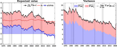
Our framework allows us to study the characteristics of the conditional distributions of GDP growth. Figure 2 reports the time-varying mean and volatility of these distributions, which can be computed as (see, e.g., Gómez, Torres, and Bolfarine 2007) (10) $$\begin{array}{c}\mathbb{E}\left[y_t\right|\theta ,{\mathcal{Y}}^{t-1}]={\mu }_t+g(\eta ){\sigma }_t{\varrho }_t,\\ \hspace{1em}g(\eta )=\frac{4\mathcal{C}(\eta )}{1-\eta },\end{array}$$(10) (11) $$\begin{array}{c}\mathbb{V}\text{ar}(y_t|\theta ,{\mathcal{Y}}^{t-1})={\sigma }_t^2(\frac{1}{1-2\eta }+h(\eta ){\varrho }_t^2),\\ \hspace{1em}h(\eta )=\frac{3}{1-2\eta }-g{(\eta )}^2.\end{array}$$(11)

Fig. 2 Time-varying mean and variance.

NOTE: The plots illustrate the time-varying mean and standard deviation (blue), along with the respective long-run components, in red, and 90% credible intervals. Shaded bands represent NBER recessions.

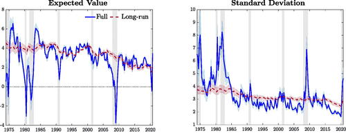
The mean moves along the business cycle, sharply contracting during recessions, while volatility is markedly countercyclical, with peaks occurring during recessions. Focusing on the last year of the sample, volatility sharply increases and the mean rebounds quickly, suggesting that Covid-quarters are, at least partially, characterized as tail events. We also report, in red, the low-frequency components, that is the moments of the distribution that would prevail in the absence of any transitory variation of the parameters. These capture a fall in long-run growth, with the expected value falling from roughly 4% in the 1970s, to roughly 2.3% at the end of the sample. The Great Moderation is reflected in a reduction of GDP growth’s volatility: starting in the mid-1980s, transitory fluctuations in volatility dampen down as the impact of the consecutive recessions of the 1970s and 1980s fades away, and the long-run volatility is revised downward by about 30%.

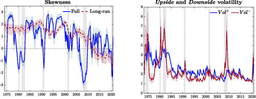
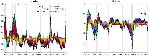
Time-varying skewness is reported in the left panel of Figure 3.¹⁴ This evolves in a procyclical fashion, such that substantially negative skewness characterizes recessions, whereas expansions are marked by positively skewed distributions. Interestingly, skewness tends to decrease in anticipation of recessions, a feature which we show to be related to the information contained in the financial indicators, suggesting that downside risk dominates ahead of, and during downturns. Over the long-run, skewness displays a downward trend starting in the late 1980s, and falling markedly in the post-2000 sample. As a result, business cycle fluctuations feature decreasing, but positive, trend-skewness until the onset of the financial crisis in 2007. In the aftermath of the subsequent recession, this trend turns negative, implying negatively skewed long-run conditional distributions. This signals the build-up of vulnerabilities, resulting in the economy being increasingly exposed to downside risks.

Fig. 3 Time-varying asymmetry.

NOTE: The left panel illustrates the estimated time-varying moment skewness (blue), along with its long-run component (red). The right panel reports the upside and downside volatilities, in blue and red, respectively. Shadings correspond to 90% credible intervals. Shaded bands represent NBER recessions.

4.1 Upside and Downside Volatility

In line with the “good” and “bad” volatility decomposition of Bekaert and Engstrom (2017), we define “upside” ($Vo{l}^{+}=\sqrt{\mathbb{V}\text{ar}(y_t|y_t\ge {\mu }_t)}$) and “downside” ($Vo{l}^{-}=\sqrt{\mathbb{V}\text{ar}(y_t|y_t<{\mu }_t)}$) volatility as a function of ϱ (see Appendix B): (12) $$\begin{array}{c}Vo{l}^{+}=\frac{1+{\varrho }_t}{2}\sqrt{\mathbb{V}\text{ar}(y_t|\theta ,{\mathcal{Y}}^{t-1})},\\ Vo{l}^{-}=\frac{1-{\varrho }_t}{2}\sqrt{\mathbb{V}\text{ar}(y_t|\theta ,{\mathcal{Y}}^{t-1})}.\end{array}$$(12)

These two components are reported in the right panel of Figure 3. Downside volatility spikes during recessions, whereas upside volatility displays only modest (pro-)cyclicality. Therefore, the countercyclicality of aggregate volatility (see, e.g., Jurado, Ludvigson, and Ng 2015) largely reflects transitory developments in downside risks. While the financial crisis appears as an episode of pure downside risk, the recent Covid-recession featured a spike in downside volatility in the first half of 2020, swiftly receding in favor of upside risks in the second half.

4.2 Expected Value and Variance Decomposition

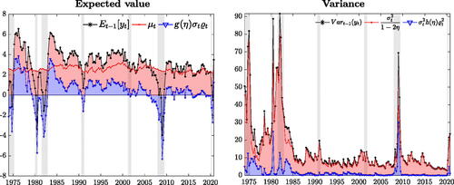
Fluctuations in the conditional skewness of GDP growth plays an important role in determining the dynamics of the first and second moments of the conditional distributions (see (10) and (11)). Thus, the (time-varying) expected value and variance are equal to those of a standard t distribution, plus a component which is a function of the shape parameter. The impact of the asymmetry on the conditional mean is magnified by larger values of σ_t and it disappears when ${\varrho }_t=0$.

Figure 4 isolates the contribution of the asymmetry in the first and second moments. The location (red) is remarkably stable over the sample, such that most of the fluctuations in the expected value reflect shifts of the shape parameter (blue), with recessions (expansions) characterized by negative (positive) skewness. The contribution of the asymmetry for positive expected values becomes more muted during the Great Moderation, whereas the negative drag from the asymmetry remains important during recessions. In contrast, the effect of $\left|{\varrho }_t\right|$ on the second moment is less pervasive, despite deepening skewness during recessions accounts for a nontrivial share of the increase in variance.

Fig. 4 Expected value and variance decomposition.

NOTE: The plot shows the decomposition of the expected value and variance of GDP growth. Location and scale are reported in red, while the contribution of higher order moments is in blue. Central moments (black) are computed as in (10) and (11). Shaded bands represent NBER recessions.

Equations (10)(10) $$\begin{array}{c}\mathbb{E}\left[y_t\right|\theta ,{\mathcal{Y}}^{t-1}]={\mu }_t+g(\eta ){\sigma }_t{\varrho }_t,\\ \hspace{1em}g(\eta )=\frac{4\mathcal{C}(\eta )}{1-\eta },\end{array}$$(10) and (11)(11) $$\begin{array}{c}\mathbb{V}\text{ar}(y_t|\theta ,{\mathcal{Y}}^{t-1})={\sigma }_t^2(\frac{1}{1-2\eta }+h(\eta ){\varrho }_t^2),\\ \hspace{1em}h(\eta )=\frac{3}{1-2\eta }-g{(\eta )}^2.\end{array}$$(11) also highlight that procyclical variations of skewness are reflected into a time-varying correlation between the mean and the volatility. The mean is positively affected by shifts of the shape parameter, $\frac{\partial \mathbb{E}(y_t|\theta ,{\mathcal{Y}}^{t-1})}{\partial {\varrho }_t}>0,\forall {\varrho }_t$. When ${\varrho }_t$ increases, the variance increases (decreases) if the distribution is positively (negatively) skewed, as $\frac{\partial \mathbb{V}\text{ar}(y_t|\theta ,{\mathcal{Y}}^{t-1})}{\partial {\varrho }_t}=2h(\eta ){\sigma }_t^2{\varrho }_t$ and $h(\eta )>0$, in that the distribution becomes more asymmetric. Therefore, procyclical skewness reduces volatility during expansions, and increases it during recessions. These nonlinearities in the interaction between uncertainty and aggregate economic activity are consistent with findings in Segal, Shaliastovich, and Yaron (2015), that “positive uncertainty” is associated with positive (conditional) expected growth, whereas this correlation turns negative during contractions.

4.3 Long-Run Growth Slowdown and the Great Moderation

We use (10) and (11) to assess the properties of long-run growth. Figure 5 shows that the decreasing skewness-trend maps into a decline of long-run growth, as roughly two thirds of this slowdown reflect a reassessment of risk. The downward trend in long-run growth is temporarily reversed in correspondence of the IT productivity boom of the mid-1990s, when growth is revised upward by roughly 0.5%. This upward revision reflects, to a large extent, a shift in upside risk to GDP growth. In the post-2000, the slowdown in long-run growth accelerates, along with a rebalancing of risks toward the downside. After the Great Recession, long-run growth displays a pronounced left tail, thus becoming a negative drag to long-term growth.

Fig. 5 Long-run GDP growth and volatility.

NOTE: The left plot shows the contribution of the long-run location ${\overline{\mu }}_t$ (red), and of higher order moments (blue) to the long-run expected value (black). Similarly, we decompose the total long-run variance (black) into upside (blue) and downside (red) variance. Shaded bands represent NBER recessions.

Similarly, we decompose long-run variance into the contributions of long-run upside (blue) and downside (red) variance in the right panel of Figure 5. Upside variance decreases over the Great Moderation period, and by the end of the sample it has halved with respect to its level in the 1970s. On the contrary, the downside component has remained quite stable throughout the sample. This highlights that the Great Moderation reflects a reduction in upside risk not matched by an equal fall in downside risk (in line with Jensen et al. 2020).

4.4 Conditional versus Unconditional Skewness

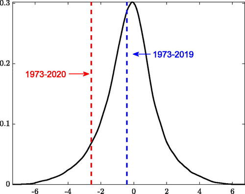
Figure 3 highlights that the skewness of the conditional distribution displays a marked procyclicality: expansions are characterized by right-skewness, whereas contractions are associated with negatively-skewed distributions. What does this mean for the unconditional distribution of GDP growth? We answer this question by drawing inference on the unconditional (a)symmetry of the data. We simulate 10,000 alternative paths of GDP growth from the estimated model, and we compute the associated (unconditional) skewness. The results are summarized in Figure 6. Negative unconditional skewness estimates turn out to be 20% more likely than positive estimates, despite conditional distributions displaying positive skewness for a large part of the sample. During expansions upside volatility is, on average, 15% higher than downside volatility, while the latter is almost double the former during recessions (see Figure 3). Thus, despite expansions being typically characterized by right-skewed conditional distributions, the occurrence of tail events is impaired by lower dispersion. Differently, recessions are characterized by higher downside uncertainty, resulting in large negative observations being more likely. For the 1973–2019 period, sample skewness value of–0.42 lies close to the expected value of the empirical distribution; the sample skewness of–2.58 due to the Pandemic-recession still lies well within the 95% interval. Results are not affected by omitting 2020 from the sample. Testing the unconditional skewness on simulated data fails to find significant evidence of any degree of asymmetry. Therefore, significant variation of the conditional skewness over the sample does not prevent the model from generating unconditionally symmetric distribution of GDP growth, consistent with what we find in the data.

Fig. 6 Unconditional skewness.

NOTE: The figure reports the distribution of the unconditional skewness, obtained from 10,000 paths of GDP growth simulated from the model. The vertical lines indicate the unconditional skewness estimated over two alternative samples.

4.5 The Contribution of Financial Predictors

To gauge the contribution of financial indicators to the variation of the parameters, we exploit the moving average representation of the transitory components ${\tilde{\gamma }}_t$ and ${\tilde{\delta }}_t$, and decompose them into a “score-driven” component (${\kappa }_{\gamma }{\sum }_{j=0}^{t-1}{\varphi }_{\gamma }^j{s}_{\gamma t-j}$ and ${\kappa }_{\delta }{\sum }_{j=0}^{t-1}{\varphi }_{\delta }^j{s}_{\delta t-j}$) and a component reflecting the share of variation driven by the predictors (${\beta }_{\gamma }^{\prime }{\sum }_{j=0}^{t-1}{\varphi }_{\gamma }^j{X}_{t-j}$ and ${\beta }_{\delta }^{\prime }{\sum }_{j=0}^{t-1}{\varphi }_{\delta }^j{X}_{t-j}$), for which we highlight the contribution of each financial index (Figure 7). The dynamics of financial risks is the key driver of the countercyclical movements of the dispersion of the conditional distribution. Leverage is an important determinant of the dynamics of ${\varrho }_t$, and thus of skewness. In particular, nonfinancial leverage drives most of asymmetry’s variation, consistently with the leverage-cycle narrative of Jordà, Schularick, and Taylor (2013). The build-up of household leverage is identified as the main contributor to the increase in downside risk in the first half of the 2000s, and the subsequent deleveraging is associated with a substantial fall in downside risk. Indicators of credit spread and credit risk mainly predict the sharp increase in downside risk at the height of major recessions.

Fig. 7 Predictive financial conditions.

NOTE: The figures plot the decomposition of ${\tilde{\gamma }}_t$ and ${\tilde{\delta }}_t$ (black) into a “Score-driven” (yellow) and “Predictor-driven” components. Shaded bands represent NBER recessions.

5 Out-of-Sample Evaluation

In this Section we investigate the out-of-sample forecasting performance of our baseline model (Skt -4DFI) against a Gaussian autoregressive model with GARCH innovations, which has been proven to be a competitive benchmark for forecasting GDP growth (Clark and Ravazzolo 2015) and GDP growth-at-risk (Brownlees and Souza 2021). We also consider a Skew-t model without predictors, and a version including the NFCI. We re-estimate the models every quarter over the period 1980Q1–2020Q4, and produce one-quarter and one-year horizon forecasts; we report the latter as cumulated output growth over four quarters. Forecasts are obtained from real-time GDP vintages, and evaluated at the latest available release. We compare the performance of the models for the entire out-of-sample period, as well as for the post-2000s, and for the recessive periods in the forecasting sample.¹⁵ We assess point forecast accuracy via the mean square forecast error (MSFE). Density forecast accuracy is evaluated via the predictive log-score (logS) and quantile scores of Gneiting and Ranjan (2011). For the latter we consider (a) the Continuously Ranked Probability Score (CRPS, Gneiting and Raftery 2007), which assigns equal weight to each quantile of the empirical distribution function, and (b) a scoring rule that assigns higher weights to the lower quantiles of the distribution function (wQS), emphasizing the accuracy in predicting outcomes in left tail.¹⁶ Similarly, we evaluate the calibration of the predictive densities explicitly considering the calibration of the left side of the distributions, and we assess the models’ ability to predict tail risks and time recessions. For all measures, we report ratios (differences for the logS) with respect to the Gaussian benchmark, and we report p-values for Diebold and Mariano (1995) test, applying Harvey, Leybourne, and Newbold (1997) small sample correction.

5.1 Point, Density and Downside Risk Forecasts

5.1.1 Asymmetry and the Value of Financial Predictors

Table 2 reports the performance of competing models, for one-quarter and one-year ahead predictions. Simply introducing fat tails and time-varying asymmetry improves forecast accuracy with respect to the benchmark specification under all loss functions. Conditioning for the four financial indices leads to additional gains, in particular in the post-2000 and during recessions, over both horizons. Compared to the benchmark, Skt -4DFI produces roughly 20% (30%) improvement in MSFE, and 5% (12%) and 10% (25%) improvements in the CRPS and wQS, respectively, for the one-quarter (one-year) ahead forecasts.

Table 2 Forecasting performance.

	Skt	Skt	Skt	Skt	Skt	Skt
		NFCI	4DFI		NFCI	4DFI
	One-quarter ahead
	MSFE			logS
Full	$\underset{(0.000)}{\mathbf{0}.\mathbf{842}}$	$\underset{(0.000)}{\mathbf{0}.\mathbf{817}}$	$\underset{(0.000)}{\mathbf{0}.\mathbf{812}}$	$\underset{(0.000)}{\mathbf{0}.\mathbf{122}}$	$\underset{(0.000)}{\mathbf{0}.\mathbf{140}}$	$\underset{(0.084)}{\mathbf{0}.\mathbf{060}}$
Post ’00	$\underset{(0.000)}{\mathbf{0}.\mathbf{809}}$	$\underset{(0.000)}{\mathbf{0}.\mathbf{804}}$	$\underset{(0.000)}{\mathbf{0}.\mathbf{793}}$	$\underset{(0.000)}{\mathbf{0}.\mathbf{181}}$	$\underset{(0.000)}{\mathbf{0}.\mathbf{211}}$	$\underset{(0.001)}{\mathbf{0}.\mathbf{167}}$
Rec.	$\underset{(0.000)}{\mathbf{0}.\mathbf{831}}$	$\underset{(0.000)}{\mathbf{0}.\mathbf{807}}$	$\underset{(0.000)}{\mathbf{0}.\mathbf{795}}$	$\underset{(0.034)}{\mathbf{0}.\mathbf{227}}$	$\underset{(0.056)}{\mathbf{0}.\mathbf{265}}$	$\underset{(0.269)}{0.148}$
	CRPS			wQS
Full	$\underset{(0.047)}{\mathbf{0}.\mathbf{964}}$	$\underset{(0.005)}{\mathbf{0}.\mathbf{941}}$	$\underset{(0.025)}{\mathbf{0}.\mathbf{952}}$	$\underset{(0.064)}{\mathbf{0}.\mathbf{960}}$	$\underset{(0.006)}{\mathbf{0}.\mathbf{926}}$	$\underset{(0.009)}{\mathbf{0}.\mathbf{926}}$
Post ’00	$\underset{(0.000)}{\mathbf{0}.\mathbf{934}}$	$\underset{(0.000)}{\mathbf{0}.\mathbf{912}}$	$\underset{(0.000)}{\mathbf{0}.\mathbf{918}}$	$\underset{(0.000)}{\mathbf{0}.\mathbf{919}}$	$\underset{(0.000)}{\mathbf{0}.\mathbf{894}}$	$\underset{(0.002)}{\mathbf{0}.\mathbf{891}}$
Rec.	$\underset{(0.191)}{0.961}$	$\underset{(0.135)}{0.945}$	$\underset{(0.112)}{0.938}$	$\underset{(0.030)}{\mathbf{0}.\mathbf{925}}$	$\underset{(0.030)}{\mathbf{0}.\mathbf{907}}$	$\underset{(0.019)}{\mathbf{0}.\mathbf{868}}$
	One-year ahead
	MSFE			logS
Full	$\underset{(0.000)}{\mathbf{0}.\mathbf{720}}$	$\underset{(0.002)}{\mathbf{0}.\mathbf{716}}$	$\underset{(0.003)}{\mathbf{0}.\mathbf{694}}$	$\underset{(0.000)}{\mathbf{0}.\mathbf{486}}$	$\underset{(0.000)}{\mathbf{0}.\mathbf{585}}$	$\underset{(0.001)}{\mathbf{0}.\mathbf{518}}$
Post ’00	$\underset{(0.000)}{\mathbf{0}.\mathbf{720}}$	$\underset{(0.000)}{\mathbf{0}.\mathbf{696}}$	$\underset{(0.002)}{\mathbf{0}.\mathbf{718}}$	$\underset{(0.000)}{\mathbf{0}.\mathbf{849}}$	$\underset{(0.000)}{\mathbf{0}.\mathbf{978}}$	$\underset{(0.000)}{\mathbf{0}.\mathbf{970}}$
Rec.	$\underset{(0.063)}{\mathbf{0}.\mathbf{743}}$	$\underset{(0.163)}{0.764}$	$\underset{(0.044)}{\mathbf{0}.\mathbf{656}}$	$\underset{(0.004)}{\mathbf{1}.\mathbf{071}}$	$\underset{(0.007)}{\mathbf{1}.\mathbf{209}}$	$\underset{(0.015)}{\mathbf{1}.\mathbf{238}}$
	CRPS			wQS
Full	$\underset{(0.003)}{\mathbf{0}.\mathbf{912}}$	$\underset{(0.002)}{\mathbf{0}.\mathbf{902}}$	$\underset{(0.003)}{\mathbf{0}.\mathbf{883}}$	$\underset{(0.001)}{\mathbf{0}.\mathbf{778}}$	$\underset{(0.001)}{\mathbf{0}.\mathbf{747}}$	$\underset{(0.005)}{\mathbf{0}.\mathbf{766}}$
Post ’00	$\underset{(0.000)}{\mathbf{0}.\mathbf{843}}$	$\underset{(0.000)}{\mathbf{0}.\mathbf{826}}$	$\underset{(0.000)}{\mathbf{0}.\mathbf{820}}$	$\underset{(0.000)}{\mathbf{0}.\mathbf{725}}$	$\underset{(0.000)}{\mathbf{0}.\mathbf{703}}$	$\underset{(0.000)}{\mathbf{0}.\mathbf{711}}$
Rec.	$\underset{(0.193)}{0.942}$	$\underset{(0.316)}{0.957}$	$\underset{(0.099)}{\mathbf{0}.\mathbf{890}}$	$\underset{(0.008)}{\mathbf{0}.\mathbf{725}}$	$\underset{(0.028)}{\mathbf{0}.\mathbf{737}}$	$\underset{(0.016)}{\mathbf{0}.\mathbf{668}}$

The table reports the average forecast scores relative to the Gaussian model. Positive logS differences, and ratios smaller than 1 for the MSFE, CRPS, and wQS indicate that the column-specific model performs better than the benchmark. The p-values for equal forecast accuracy are in parentheses. Values in bold are significant at the 10% level; gray shaded cells highlight the best score. Out-of-sample periods: Full, 1980Q1–2020Q4; Post’00, 2000Q1–2020Q4; Rec., three quarters before and after NBER recession dates.

5.1.2 Comparison with Adrian, Boyarchenko, and Giannone (2019)

In Table 3 we report the comparison of the baseline specification against the model of Adrian, Boyarchenko, and Giannone (2019).¹⁷ Our baseline specification is associated with better point and density forecasts, and with significant improvements, especially in the post-2000s sample. These gains, especially during recessions, stem from the adaptiveness of the score filter, which allows the shape parameter to promptly adapt to turning points, thus, generating longer left tails during downturns. In fact, compared to the model of Adrian, Boyarchenko, and Giannone (2019), the Skt -4DFI specification appears to be faster and more precise in capturing increases (decreases) in downside (upside) risk ahead of recessions, and it adapts to the subsequent rebounds in GDP growth in a more timely manner.

Table 3 Forecast performance with respect to Adrian, Boyarchenko, and Giannone (2019).

	One-quarter ahead				One-year ahead
	MSFE	logS	CRPS	wQS	MSFE	logS	CRPS	wQS
Full	$\underset{(0.000)}{\mathbf{0}.\mathbf{890}}$	$\underset{(0.000)}{\mathbf{2}.\mathbf{473}}$	$\underset{(0.221)}{0.983}$	$\underset{(0.599)}{1.006}$	$\underset{(0.562)}{1.014}$	$\underset{(0.000)}{\mathbf{0}.\mathbf{571}}$	$\underset{(0.425)}{0.989}$	$\underset{(0.672)}{1.026}$
Post ’00	$\underset{(0.000)}{\mathbf{0}.\mathbf{837}}$	$\underset{(0.000)}{\mathbf{4}.\mathbf{499}}$	$\underset{(0.000)}{\mathbf{0}.\mathbf{920}}$	$\underset{(0.006)}{\mathbf{0}.\mathbf{941}}$	$\underset{(0.098)}{\mathbf{0}.\mathbf{894}}$	$\underset{(0.000)}{\mathbf{0}.\mathbf{436}}$	$\underset{(0.046)}{\mathbf{0}.\mathbf{902}}$	$\underset{(0.224)}{0.944}$
Rec.	$\underset{(0.000)}{\mathbf{0}.\mathbf{877}}$	$\underset{(0.000)}{\mathbf{8}.\mathbf{567}}$	$\underset{(0.111)}{0.962}$	$\underset{(0.197)}{0.966}$	$\underset{(0.649)}{1.073}$	$\underset{(0.015)}{\mathbf{1}.\mathbf{407}}$	$\underset{(0.332)}{0.948}$	$\underset{(0.425)}{0.975}$

The table reports the average forecast scores of the Skt -4DFI model relative to Adrian, Boyarchenko, and Giannone (2019). Positive values of logS differences, and ratios smaller than 1 for the MSFE, CRPS, and wQS indicate that the Skt -4DFI model performs better than Adrian, Boyarchenko, and Giannone (2019). The p-values for equal forecast accuracy are in parentheses. Values in bold are significant at the 10% level. Out-of-sample periods: Full, 1980Q1–2020Q4; Post’00, 2000Q1–2020Q4; Rec., three quarters before and after NBER recession dates.

5.1.3 Density Calibration

Table 4 evaluates the calibration of the density forecasts. Berkowitz (2001) highlights that the Normal transform of the probability integral transforms (PITs) of correctly calibrated predictive densities is standard Normal, and it is independent at the one-step ahead. The upper part of Table 4 reports the estimates of the mean and variance of the normal transforms of the PITs, their autocorrelation coefficient for the one-quarter ahead, and the p-values associated with the relevant null hypotheses. Both the Gaussian specification and the model of Adrian, Boyarchenko, and Giannone (2019) overestimate, on average, upside risk one-quarter ahead, while producing overly disperse densities at the one-year horizon. Our baseline model, on the other hand, does not display any sign of miscalibration. The remainder of Table 4 reports the test statistics of Rossi and Sekhposyan (2019) test for the correct calibration of the forecast distributions, evaluated over the full densities, the left-half and the left-tail. The test rejects the null hypothesis of correctly calibrated densities for both competing models, at both horizons. In contrast, our baseline model delivers well calibrated forecasts for the entire density, as well as for the left part of the predictive distributions, capturing movements in downside risk.

Table 4 Density calibration tests.

			Skt			Skt
	AR(2)	ABG	4DFI	AR(2)	ABG	4DFI
PITs:	One-quarter ahead			One-year ahead
Mean	$\underset{(0.000)}{-\mathbf{0}.\mathbf{352}}$	$\underset{(0.028)}{-\mathbf{0}.\mathbf{238}}$	$\underset{(0.755)}{0.030}$	$\underset{(0.000)}{-\mathbf{0}.\mathbf{941}}$	$\underset{(0.248)}{-0.225}$	$\underset{(0.951)}{0.011}$
Var	$\underset{(0.801)}{0.963}$	$\underset{(0.904)}{0.983}$	$\underset{(0.745)}{1.041}$	$\underset{(0.007)}{\mathbf{2}.\mathbf{009}}$	$\underset{(0.001)}{\mathbf{2}.\mathbf{071}}$	$\underset{(0.125)}{1.290}$
AR(1)	$\underset{(0.742)}{-0.026}$	$\underset{(0.028)}{\mathbf{0}.\mathbf{171}}$	$\underset{(0.126)}{0.120}$
						RS test:
Full	$\underset{}{\mathbf{2}.\mathbf{102}}$	$\underset{}{\mathbf{1}.\mathbf{925}}$	$\underset{}{0.883}$	$\underset{}{\mathbf{4}.\mathbf{865}}$	$\underset{}{\mathbf{2}.\mathbf{306}}$	$\underset{}{1.162}$
Left-half	$\underset{}{\mathbf{1}.\mathbf{798}}$	$\underset{}{\mathbf{1}.\mathbf{415}}$	$\underset{}{0.805}$	$\underset{}{\mathbf{4}.\mathbf{865}}$	$\underset{}{\mathbf{2}.\mathbf{306}}$	$\underset{}{1.162}$
Left tail	$\underset{}{\mathbf{1}.\mathbf{074}}$	$\underset{}{\mathbf{1}.\mathbf{166}}$	$\underset{}{0.501}$	$\underset{}{\mathbf{4}.\mathbf{757}}$	$\underset{}{\mathbf{2}.\mathbf{306}}$	$\underset{}{1.162}$

The table reports the mean and variance of the normal transform of the PITs, and the coefficient of an AR(1) model estimated on the one-step ahead transform. We report in parentheses the p-values, computed with HAC variances, for the null of zero mean and unit variance of the normalized forecasts, and we test the null of no persistence for the one-step ahead. We also report Rossi and Sekhposyan (2019, RS) calibration tests, considering the full density support (Full), the left-half, defined over the [0 0.5] support, and the left-tail, over the support [0, 0.25]. Values in bold indicate the rejection of the null hypothesis at the 10% confidence level. Critical values for the RS tests are obtained by 1000 bootstrap simulations.

5.2 Tail Risk Predictions

Measures such as Value at Risk (VaR), as well as the Expected Shortfall (ES), are readily obtained within our framework. $E{S}_{t+h}^{\alpha }={\alpha }^{-1}{\int }_0^{\alpha }Va{R}_{t+h|t}^{a}da$ describes the expected growth level for $y_{t+h}<Va{R}_{t+h}^{\alpha }$, corresponding to the $(100\alpha )$th percentile of the h-step ahead predictive distribution, whereas the Expected Longrise (EL) is the upper counterpart of the ES. 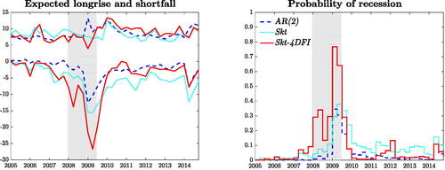The left hand panel of Figure 8 contrasts the $E{S}^{5\%}$ and the $E{L}^{95\%}$ for the Gaussian model, the Skt model without financial predictors and our baseline model, considering 10 years around the financial crisis. The Gaussian model fails to capture the building-up of risk ahead of the Great Recession, predicting an ES around zero as the economy enters the recession. In addition, assuming a symmetric distribution implies that a fall in the ES is often associated with peaks in the EL. In that, the minimum ES corresponds to the maximum EL in 2009Q2. Allowing for Skew-t innovations alleviates both problems, delivering more conservative risk measures, with less erratic longrise figures and anticipating the build-up of downside risk ahead of the recession. Conditioning the forecasts on financial conditions increases the timeliness of the prediction of risk, due to the prompt discounting of financial overheating. The prediction of the ES falls to roughly–5% in the first quarter of the recessions, and decreases consistently until the first quarter of recovery, when it is sharply revised upwards. Timely updates of the asymmetry parameter, especially at turning points, induce a reduction in the mean and an increase in downside risk.¹⁸

Fig. 8 Expected shortfall and expected longrise.

NOTE: We report the ${\text{ES}}^{5\%}$ and ${\text{EL}}^{95\%}$. Probabilities of recessions are computed as the probability of observing two consecutive negative growth forecasts over the next four quarters. Shaded bands represent NBER recessions.

Brownlees and Souza (2021) argue that a GARCH model provides competitive out-of-sample forecasts for the lower quantiles of the GDP growth distribution. In Table 5 we show that allowing for time-varying skewness produces large and significant gains with respect to the Gaussian model, with improvements of 35% at the one-quarter ahead horizon, and up to 70% at the one-year ahead. These results remains robust to different scoring functions.

Table 5 Tail risk scores.

	Skt	Skt	Skt	Skt	Skt	Skt
	no-X	4DFI	no-X	4DFI	no-X	4DFI
	FZG		ALS		TLF
	One-quarter ahead
Full	$\underset{(0.040)}{\mathbf{0}.\mathbf{831}}$	$\underset{(0.028)}{\mathbf{0}.\mathbf{819}}$	$\underset{(0.111)}{0.959}$	$\underset{(0.028)}{\mathbf{0}.\mathbf{948}}$	$\underset{(0.246)}{0.978}$	$\underset{(0.003)}{\mathbf{0}.\mathbf{900}}$
Post ’00	$\underset{(0.002)}{\mathbf{0}.\mathbf{693}}$	$\underset{(0.003)}{\mathbf{0}.\mathbf{720}}$	$\underset{(0.012)}{\mathbf{0}.\mathbf{912}}$	$\underset{(0.038)}{\mathbf{0}.\mathbf{926}}$	$\underset{(0.066)}{\mathbf{0}.\mathbf{943}}$	$\underset{(0.040)}{\mathbf{0}.\mathbf{915}}$
Rec.	$\underset{(0.014)}{\mathbf{0}.\mathbf{741}}$	$\underset{(0.013)}{\mathbf{0}.\mathbf{651}}$	$\underset{(0.030)}{\mathbf{0}.\mathbf{880}}$	$\underset{(0.044)}{\mathbf{0}.\mathbf{850}}$	$\underset{(0.072)}{\mathbf{0}.\mathbf{925}}$	$\underset{(0.012)}{\mathbf{0}.\mathbf{821}}$
	One-year ahead
Full	$\underset{(0.000)}{\mathbf{0}.\mathbf{241}}$	$\underset{(0.001)}{\mathbf{0}.\mathbf{310}}$	$\underset{(0.000)}{\mathbf{0}.\mathbf{397}}$	$\underset{(0.000)}{\mathbf{0}.\mathbf{424}}$	$\underset{(0.002)}{\mathbf{0}.\mathbf{692}}$	$\underset{(0.002)}{\mathbf{0}.\mathbf{622}}$
Post ’00	$\underset{(0.001)}{\mathbf{0}.\mathbf{246}}$	$\underset{(0.003)}{\mathbf{0}.\mathbf{371}}$	$\underset{(0.000)}{\mathbf{0}.\mathbf{361}}$	$\underset{(0.001)}{\mathbf{0}.\mathbf{398}}$	$\underset{(0.003)}{\mathbf{0}.\mathbf{727}}$	$\underset{(0.003)}{\mathbf{0}.\mathbf{600}}$
Rec.	$\underset{(0.000)}{\mathbf{0}.\mathbf{192}}$	$\underset{(0.000)}{\mathbf{0}.\mathbf{300}}$	$\underset{(0.000)}{\mathbf{0}.\mathbf{263}}$	$\underset{(0.000)}{\mathbf{0}.\mathbf{308}}$	$\underset{(0.000)}{\mathbf{0}.\mathbf{551}}$	$\underset{(0.003)}{\mathbf{0}.\mathbf{495}}$

The table reports the average downside tail risk scores, expressed as ratios relative to the Gaussian model. Ratios smaller than 1 indicate that the column-specific model performs better than the benchmark. The p-values for equal forecast accuracy are reported in parentheses. Values in bold are significant at the 10% level; gray shaded cells highlight the best score. FZG: Fissler, Ziegel, and Gneiting (2016) loss function; ALS: Taylor (2019) loss function; TLF: Giacomini and Komunjer (2005) tick loss function. Out-of-sample periods: Full, 1980Q1–2020Q4; Post’00, 2000Q1–2020Q4; Rec., three quarters before and after NBER recession dates.

We also investigate the ability of the model to predict recessions, which we define as the probability of observing any two consecutive negative forecasts over the next four quarters. The right panel of Figure 8 highlights that combining financial conditions and conditional asymmetry produces a realistic assessment of the risk of recession. Compared to the other models, the probability of recession produced by the Skt -4DFI specification starts picking up earlier, warning against an imminent output contraction, and it sharply recedes at the end of the recession, being already below 5% in 2009Q3. Unreported Brier scores highlight that deviating from the Gaussian assumption provides gains of around 10% in timing recessions, and an additional 20% gain can be directly ascribed to the inclusion of financial predictors. Overall, these results underline the importance of allowing for time variation in the skewness of the conditional distribution of GDP growth for predicting downside risk, both in terms of magnitude and timing.

5.3 Robustness

Here, we provide a summary of additional robustness exercises, reported in Appendix H. Using lagged GDP growth as additional predictor of the time-varying parameters leads to weaker forecast performance. Explicitly accounting for parameters’ uncertainty in the forecast delivers significant gains in terms of both point and density forecast. We show that the results reported above are robust to the exclusion of 2020 from the sample, and to the targeting of different GDP releases. We also show that the gains are associated with the time variation in asymmetry, as opposed to the presence of unconditional asymmetry. Lastly, we show that our gains are not distorted by the use of the latest vintages of the NFCI as opposed the real-time data, only available from 2013.

6 Dissecting the Financial Condition Index

We investigate whether the predictive power of the model can be further improved by considering the full set of 105 indicators of financial activity that constitute the NFCI. In particular, we use the individual contributions to the NFCI, as made available by the Chicago Fed, which measure how each individual indicator contributes to the aggregate NFCI. We start our forecasting exercise at the beginning of the 2000s, and at each point in time, we only consider indicators for which at least four years of data are available. Hence, the first forecast we produced relies on about 70% of the total available indicators, and we reach approximately 85% around the 2007–2009 recession.¹⁹

6.1 Variables Selection: “shrink-then-sparsify”

A potential concern of this exercise lies in the steep increase in the number of parameters our model needs to accommodate. We tackle this dimensionality problem through a “shrink-then-sparsify” strategy (see, e.g., Hahn and Carvalho 2015, and Appendix D.2). Shrinkage is achieved by means of Horseshoe (HS) priors: $b_i\sim \mathcal{N}(0,{\lambda }_i\tau )$, where the hyperparameters λ_i and τ control the local and the global shrinkage of the predictor loadings, respectively. Specifically, ${\lambda }_i\sim H{C}^{+}(0,1)$ and $\tau \sim H{C}^{+}(0,1)$, where $H{C}^{+}(0,1)$ denotes the standard Half-Cauchy distribution. Unlike other common shrinkage priors (e.g., Ridge, Lasso), HS priors are free of exogenous inputs, implying a fully adaptive shrinkage procedure. We then apply the Signal Adaptive Variable Selector (SAVS) algorithm of Ray and Bhattacharya (2018) to reduce the estimation uncertainty associated with the shrinkage. This data-driven procedure specifies the sparsification tuning parameter as $m_i=|{\widehat{b}}_i{|}^{-2}$ such that each predictor i receives a penalization “ranked in inverse-squared order of magnitude of the corresponding coefficient” (Ray and Bhattacharya 2018). Thus, (13) $$b_i^{*}=\text{sgn}({\widehat{b}}_i)||X_j|{|}^{-2}\max \{|{\widehat{b}}_i|·||X_j|{|}^2-m_i,0\},$$(13) where $||·||$ represents the Euclidean norm of the vector X_j . Note that by applying the sparsification step at each draw of the MCMC algorithm, the approach fully accounts for model uncertainty, akin to the idea of Bayesian model averaging (Huber, Koop, and Onorante 2021).

6.2 On the Importance of Financial Indicators

Table 6 reports the forecasting performance of the sparse model, based on the $b_j^{*}$ coefficients, against our baseline specification (Skt -4DFI), over the full sample (2000–2020), the 2000–2019 sample, and all the post-2000 recessions. Over the full sample, the sparse model realizes gains of up to 10% (12%) in point (density) forecast accuracy, at the one-quarter-ahead; these translate into gains up to 25% (20%) with respect to the Gaussian benchmark.

Table 6 Sparse forecast performance.

	One-quarter ahead				One-year ahead
	MSFE	logS	CRPS	wQS	MSFE	logS	CRPS	wQS
Full	$\underset{(0.000)}{\mathbf{0}.\mathbf{900}}$	$\underset{(0.000)}{\mathbf{0}.\mathbf{327}}$	$\underset{(0.000)}{\mathbf{0}.\mathbf{896}}$	$\underset{(0.000)}{\mathbf{0}.\mathbf{883}}$	$\underset{(0.214)}{1.003}$	$\underset{(0.075)}{\mathbf{0}.\mathbf{239}}$	$\underset{(0.160)}{0.954}$	$\underset{(0.310)}{0.943}$
Pre-2020	$\underset{(0.012)}{\mathbf{0}.\mathbf{899}}$	$\underset{(0.001)}{\mathbf{0}.\mathbf{100}}$	$\underset{(0.003)}{\mathbf{0}.\mathbf{915}}$	$\underset{(0.010)}{\mathbf{0}.\mathbf{907}}$	$\underset{(0.518)}{0.940}$	$\underset{(0.355)}{0.082}$	$\underset{(0.348)}{0.964}$	$\underset{(0.648)}{0.965}$
Rec.	$\underset{(0.000)}{\mathbf{0}.\mathbf{906}}$	$\underset{(0.000)}{\mathbf{0}.\mathbf{716}}$	$\underset{(0.000)}{\mathbf{0}.\mathbf{897}}$	$\underset{(0.002)}{\mathbf{0}.\mathbf{890}}$	$\underset{(0.968)}{0.935}$	$\underset{(0.807)}{0.312}$	$\underset{(0.896)}{1.011}$	$\underset{(0.972)}{1.005}$

The table reports the average forecast scores from the sparse model relative to the Skt -4DFI. Positive values of logS differences, and ratios smaller than 1 for the MSFE, CRPS, and wQS indicate that the sparse model performs better than Skt -4DFI. The p-values for equal forecast accuracy are in parentheses. Values in bold are significant at the 10% level. Out-of-sample periods: Full, 1980Q1–2020Q4; Post’00, 2000Q1–2020Q4; Rec., three quarters before and after NBER recession dates.

These performances are only slightly affected by 2020, suggesting the model is well suited to cope with such extraordinary realizations. Looking at the cumulative sums of the relative forecast scores it emerges that the sparse model gains advantage over the Skt -4DFI throughout the entire sample and, especially, during the second quarter of 2020, where the model is able to timely capture the fall in GDP and the surrounding uncertainty. Large gains are documented during recessions, indicating that closely monitoring financial market distress can improve the assessment of macroeconomic (downside) risk ahead and during times of crisis, in line with Alessi et al. (2014).

We further investigate the importance of sparsity when relying on a large number of predictors. Specifically, we compare the sparse model to a “dense” specification, where the SAVS step is omitted. The sparse model is associated with large gains in forecasting performance under any loss function pointing at the importance of reducing estimation uncertainty relative to the predictors’ loadings in a large data setting (see Appendix I).

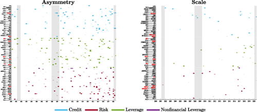
In Figure 9 we illustrate the evolution of sparsity in the financial information set over time, for the asymmetry and scale parameters. Financial information appears to be more informative for capturing the time variation of the asymmetry parameter, rather than the scale, and for both we observe a decreasing pattern in sparsity. On average, about 7.5% of the predictors feed into the prediction of the asymmetry parameter, while only about 2% contribute to the scale; toward the end of the sample, more than 10% of the indicators inform the asymmetry parameter, while only 5% relate to σ_t . During the financial crisis we document a decrease in sparsity for ${\varrho }_t$, highlighting the importance of monitoring developments in financial markets to gauge the severity of the Great Recession. Ranking predictors by their average posterior probability of inclusion shows that leverage indicators provide most of the information relevant to predict the evolution of the asymmetry parameter, along with credit conditions and household debt. Credit spreads appear most informative for the scale parameter. In line with the narrative in Adrian and Shin (2008), during the Global Financial Crisis the size of the shadow-banking sector, and the issuance of mortgage-backed securities, provide useful signals to gauge increasing downside risks.

Fig. 9 Sparsity.

NOTE: The panels reports the evolution of the financial predictors selected for the asymmetry and scale parameters. Names in red indicate the 10 predictors with the highest posterior probability of inclusion (pip); names in bold indicates predictors with the highest pip around the Global Financial Crisis.

7 Conclusions

The severity of the latest financial crisis and the ensuing recession has spurred the interest of both academics and practitioners in developing models that allow us to better understand and predict downside risk to economic growth. We introduce a framework that allows to characterize permanent and transitory variation of the whole conditional distribution of GDP growth, ensuring robustness to tail events and delivering competitive out-of-sample (point, density and tail) forecasts. Our model highlights how the properties of GDP growth have changed over the last 50 years. Downside risks have steadily increased, adversely affecting long-run growth. The fall in volatility observed since the mid-1980s reflects a substantial fall in upside volatility, with downside volatility remaining relatively stable over the entire sample. Procyclical skewness emerges as a strong feature of the data, which strongly relates to leverage developments and credit availability. When financial markets are overheating, future economic growth becomes more uncertain, and downside risk arises, reflecting the negative skewness of the predictive distributions of GDP growth.

Acknowledgments

This article is extracted from the first chapter of the Ph.D. thesis of Andrea De Polis at the University of Warwick. We thank three referees, the editor and associate editor, Jesús Fernández-Villaverde for the thoughtful discussion and Domenico Giannone and Elmar Mertens for extensive comments on an earlier draft of the article. We also thank Anastasia Allayioti, Scott Brave, Christian Brownlees, Andrew Butters, Andrea Carriero, Todd Clark, Gabriele Fiorentini, Ana Galvao, Francesco Saverio Gaudio, Gary Koop, André Lucas, Massimiliano Marcellino, Leonardo Melosi, James Mitchell, Mikkel Plagborg-Møller, Bernd Schwaab, Andreas Tryphonides, Fabrizio Venditti, Mark Watson and the participants at various conferences and seminars where the article was presented for valuable feedback and suggestions. We are grateful to the Chicago FED for making the full panel of weighted contribution of the financial indicators available for this work. The views expressed in this manuscript are those of the authors and do not necessarily reflect the views of the Bank of Italy. Any errors and omissions are the sole responsibility of the authors.

Supplementary Materials

The Supplemental Material reports additional results discussed throughout the paper. Appendix A provides further details on the testing procedure for time-varying conditional asymmetry, as discussed in Section 2. Appendix B offers additional details and derivations of the econometric model. Appendix C highlights the relevance of modeling time-varying asymmetry in the conditional distribution and contrasts our model with the one in Plagborg-Møller et al. (2020). Appendix D provides details on the estimation procedure. Appendix E reports the results of the Monte Carlo experiment, summarized in Section 3, and compares our model to existing ad-hoc approaches to time-varying asymmetry. Appendix F provides details about the data. Appendix G discusses in-sample model fit. Appendix H presents additional detailed results about the forecasting exercise described in Section 5. Appendix I offers additional results about the Sparse model in Section 6. Appendix J collects additional tables and figures.

Disclosure Statement

The authors report there are no competing interests to declare.

Notes

1 Huber, Koop, and Onorante (2021) note that in this setting sparsity is not an artifact of strong a priori beliefs.

2 Using the Bai and Ng (2005) test over different rolling windows, we often reject the null of symmetry, with significant negative and positive skewness detected over the sample. See Figure A.1 in Appendix A.

3 Differently from the Skew-t distribution of Azzalini and Capitanio (2003), the one of Gómez, Torres, and Bolfarine (2007) has an Information matrix which is always nonsingular, provided $|{\varrho }_t|<1$. For practical purposes, we set ${\varrho }_t=c\tanh ({\delta }_t)$, with c being a constant close but below 1, to ensure ${\varrho }_t\in (-1,1)$. This results in a small change in the Jacobian of the transformation, and is omitted to simplify the exposition.

4 In Section 3.1 we allow the time-varying parameters to feature a permanent and a transitory component.

5 Scaling the gradient by the diagonal of the Information matrix ensures that negative (positive) prediction errors translate into negative (positive) updates of the conditional location and shape, and therefore of the conditional mean. This desirable property is not always guaranteed by the full information matrix.

6 Tapia (1977) and Byrd (1978) show the “superlinear local convergence” property of Newton’s method and its diagonalization for standard optimization problems (see also Dennis and Schnabel 1996, chap. 6).

7 We choose a prior for the learning rate that limits its size, so that it (a) reduces the possibility of overshooting in the direction of the (local) optimum, and (b) assumes conservative views on parameters time variation. See Section 3.2.

8 In addition, our framework allows for non-linearities through the mapping of the predictors into the scores, further down-weighting extreme fluctuations in the data. In Appendix C we highlight that these additional features are important to recover salient features of the distribution of GDP growth.

9 Importantly, Bayesian estimators are not affected by local discontinuities, multiple local minima and flat areas of the likelihood, and they are often much easier to compute, particularly in high-dimensional settings (see, e.g., Tian, Liu, and Wei 2007; Belloni and Chernozhukov 2009).

10 Introducing priors for the coefficients governing the learning rate effectively circumvents the “pile-up” problem, often arising when time-varying parameters feature little variation (see, e.g., Stock and Watson 1998). At the same time these priors are quite conservative, implying that any evidence in favor of the time variation of permanent components reflects strong evidence in the data.

11 Intuitively, the invertibility property ensures that the effect of the initialization vanishes asymptotically and that the filter converges to a unique limit process. We derive the elements of $\frac{\partial s(f,y_t,\theta )}{\partial f{\prime }_t}$ in Appendix B.7.

12 This comes closer to the idea of defining the estimator as the maximand of the likelihood within the invertibility region (see Blasques et al. 2018, sec. 4.2).

13 This is akin to assuming a random walk specification for their law of motion. As an alternative, one could feed predictions for the explanatory variables into the model. The latter approach produces results very similar to the ones reported here.

14 The moment skewness can be computed numerically as $\mathbb{S}\mathit{kew}(y_t|\theta ,{\mathcal{Y}}^{t-1})=\frac{{\int }_{\mathbb{R}}{(y_t-\mathbb{E}[y_t|\theta ,{\mathcal{Y}}^{t-1}])}^{3}p(y_t|\theta ,{\mathcal{Y}}^{t-1})dy}{\mathbb{V}{(y_t|\theta ,{\mathcal{Y}}^{t-1})}^{\frac{3}{2}}},$ where $p(y_t|\theta ,{\mathcal{Y}}^{t-1})$ denotes the conditional density of the Skew-t distribution at time t, and the (conditional) mean and variance are computed as in (10) and (11).

15 Recessions are considered as 3 quarters before and after NBER recession quarters. See Appendix F.

16 Specifically, quantile scores are weighted by ${(1-\alpha )}^2$, where α represent the quantile.

17 For comparability, we follow exactly the procedure of Adrian, Boyarchenko, and Giannone (2019), but re-estimating the model using real-time vintages of GDP growth.

18 In Q1 of 2009, the Skt -4DFI model predicts a negative mean and substantial downside risk, whereas the Gaussian model only predicts a slightly negative growth, with a roughly symmetric assessment of the risk surrounding this prediction; see Figure J2, in Appendix J.

19 As these data are not available in real-time, we assume that at time t the set of predictors corresponds to the quarterly average of the financial indicators from the third week of the previous quarter to the second week of the current quarter. This approach mimics the information set available to the econometrician in real-time, and avoids dealing with overlapping quarters. Once a new indicator enters the model, missing observations are set to 0, while the Euclidean norm required for the sparsification step is computed on the available data (appropriately rescaled to reflect data availability).

References

- Adrian, T., Boyarchenko, N., and Giannone, D. (2019), “Vulnerable Growth,” American Economic Review, 109, 1263–89. DOI: 10.1257/aer.20161923.
- Adrian, T., Duarte, F., Liang, N., and Zabczyk, P. (2020), “NKV: A New Keynesian Model with Vulnerability,” AEA Papers and Proceedings, 110, 470–76. DOI: 10.1257/pandp.20201023.
- Adrian, T., Grinberg, F., Liang, N., Malik, S., and Yu, J. (2022), “The Term Structure of Growth-at-Risk,” American Economic Journal: Macroeconomics, Forthcoming. DOI: 10.1257/mac.20180428.
- Adrian, T., and Shin, H. S. (2008), “Financial Intermediaries, Financial Stability and Monetary Policy,” Proceedings - Economic Policy Symposium - Jackson Hole, pp. 287–334.
- Alessi, L., Ghysels, E., Onorante, L., Peach, R., and Potter, S. (2014), “Central Bank Macroeconomic Forecasting during the Global Financial Crisis: The European Central Bank and Federal Reserve Bank of New York Experiences,” Journal of Business & Economic Statistics, 32, 483–500. DOI: 10.1080/07350015.2014.959124.
- Antolin-Diaz, J., Drechsel, T., and Petrella, I. (2017), “Tracking the Slowdown in Long-Run GDP Growth,” Review of Economics and Statistics, 99, 343–356. DOI: 10.1162/REST_a_00646.
- Arellano-Valle, R. B., Gómez, H. W., and Quintana, F. A. (2005), “Statistical Inference for a General Class of Asymmetric Distributions,” Journal of Statistical Planning and Inference, 128, 427–443. DOI: 10.1016/j.jspi.2003.11.014.
- Azzalini, A., and Capitanio, A. (2003), “Distributions Generated by Perturbation of Symmetry with Emphasis on a Multivariate Skew t-distribution,” Journal of the Royal Statistical Society, Series B, 65, 367–389. DOI: 10.1111/1467-9868.00391.
- Bai, J., and Ng, S. (2005), “Tests for Skewness, Kurtosis, and Normality for Time Series Data,” Journal of Business & Economic Statistics, 23, 49–60. DOI: 10.1198/073500104000000271.
- Bekaert, G., and Engstrom, E. (2017), “Asset Return Dynamics under Habits and Bad Environment-Good Environment Fundamentals,” Journal of Political Economy, 125, 713–760. DOI: 10.1086/691450.
- Belloni, A., and Chernozhukov, V. (2009), “On the Computational Complexity of MCMC-Based Estimators in Large Samples,” The Annals of Statistics, 37, 2011–2055. DOI: 10.1214/08-AOS634.
- Berkowitz, J. (2001), “Testing Density Forecasts, With Applications to Risk Management,” Journal of Business & Economic Statistics, 19, 465–474. DOI: 10.1198/07350010152596718.
- Besag, J., Green, P., Higdon, D., and Mengersen, K. (1995), “Bayesian Computation and Stochastic Systems,” Statistical Science, 10, 3–41. DOI: 10.1214/ss/1177010123.
- Blasques, F., Gorgi, P., Koopman, S. J., and Wintenberger, O. (2018), “Feasible Invertibility Conditions and Maximum Likelihood Estimation for Observation-Driven Models,” Electronic Journal of Statistics, 12, 1019–1052. DOI: 10.1214/18-EJS1416.
- Blasques, F., Koopman, S. J., and Lucas, A. (2015), “Information-Theoretic Optimality of Observation-Driven Time Series Models for Continuous Responses,” Biometrika, 102, 325–343. DOI: 10.1093/biomet/asu076.
- Blasques, F., van Brummelen, J., Koopman, S. J., and Lucas, A. (2022), “Maximum Likelihood Estimation for Score-Driven Models,” Journal of Econometrics, 227, 325–346. DOI: 10.1016/j.jeconom.2021.06.003.
- Brave, S., and Butters, R. A. (2012), “Diagnosing the Financial System: Financial Conditions and Financial Stress,” International Journal of Central Banking, 8, 191–239.
- Brownlees, C., and Souza, A. B. (2021), “Backtesting Global Growth-at-Risk,” Journal of Monetary Economics, 118, 312–330. DOI: 10.1016/j.jmoneco.2020.11.003.
- Byrd, R. H. (1978), “Local Convergence of the Diagonalized Method of Multipliers,” Journal of Optimization Theory and Applications, 26, 485–500. DOI: 10.1007/BF00933148.
- Carriero, A., Clark, T. E., and Marcellino, M. (Forthcoming), “Capturing Macroeconomic Tail Risks with Bayesian Vector Autoregressions,” Journal of Money, Credit and Banking.
- Cecchetti, S. G. (2008), “Measuring the Macroeconomic Risks Posed by Asset Price Booms,” in Asset Prices and Monetary Policy, University of Chicago Press, NBER Chapters, 9–43.
- Chauvet, M., and Potter, S. (2013), “Forecasting Output,” in Handbook of Economic Forecasting (Vol. 2), pp. 141–194, Amsterdam: Elsevier.
- Clark, T. E., and Ravazzolo, F. (2015), “Macroeconomic Forecasting Performance under Alternative Specifications of Time-Varying Volatility,” Journal of Applied Econometrics, 30, 551–575. DOI: 10.1002/jae.2379.
- Cox, D. R. (1981), “Statistical Analysis of Time Series: Some Recent Developments,” Scandinavian Journal of Statistics, 8, 93–115.
- Creal, D., Koopman, S. J., and Lucas, A. (2013), “Generalized Autoregressive Score Models with Applications,” Journal of Applied Econometrics, 28, 777–795. DOI: 10.1002/jae.1279.
- Delle Monache, D., and Petrella, I. (2017), “Adaptive Models and Heavy Tails with an Application to Inflation Forecasting,” International Journal of Forecasting, 33, 482–501. DOI: 10.1016/j.ijforecast.2016.11.007.
- Dennis, J. E., and Schnabel, R. B. (1996), Numerical Methods for Unconstrained Optimization and Nonlinear Equations, Philadelphia, PA: Society for Industrial and Applied Mathematics.
- Diebold, F. X., and Mariano, R. S. (1995), “Comparing Predictive Accuracy,” Journal of Business & Economic Statistics, 20, 134–144. DOI: 10.1198/073500102753410444.
- Doz, C., Ferrara, L., and Pionnier, P.-A. (2020), “Business Cycle Dynamics After the Great Recession: An Extended Markov-Switching Dynamic Factor Model,” OECD Working Papers 2020/01.
- Engle, R. F., and Lee, G. (1999), “A Permanent and Transitory Component Model of Stock Return Volatility,” in Causality, and Forecasting: A Festschrift in Honor of Clive W. J. Granger, eds. R. F. Engle and H. White, pp. 475–497, Oxford: Oxford University Press.
- Engle, R. F., and Rangel, J. G. (2008), “The Spline-GARCH Model for Low-Frequency Volatility and its Global Macroeconomic Causes,” The Review of Financial Studies, 21, 1187–1222. DOI: 10.1093/rfs/hhn004.
- Eo, Y., and Morley, J. (2022), “Why Has the U.S. Economy Stagnated since the Great Recession?” The Review of Economics and Statistics, 104, 246–258. DOI: 10.1162/rest_a_00957.
- Fernández-Villaverde, J., and Guerrón-Quintana, P. (2020), “Estimating DSGE Models: Recent Advances and Future Challenges,” NBER Working Papers 27715.
- Fissler, T., Ziegel, J. F., and Gneiting, T. (2016), “Expected Shortfall is Jointly Elicitable with Value-at-Risk: Implications for Backtesting,” Risk.net.
- Ganics, G., Rossi, B., and Sekhposyan, T. (2020), “From Fixed-event to Fixed-horizon Density Forecasts: Obtaining Measures of Multi-horizon Uncertainty from Survey Density Forecasts,” CEPR Discussion Papers 14267, Centre for Economic Policy Research.
- Gertler, M., and Gilchrist, S. (2018), “What Happened: Financial Factors in the Great Recession,” Journal of Economic Perspectives, 32, 3–30. DOI: 10.1257/jep.32.3.3.
- Giacomini, R., and Komunjer, I. (2005), “Evaluation and combination of conditional quantile forecasts,” Journal of Business & Economic Statistics, 23, 416–431. DOI: 10.1198/073500105000000018.
- Giglio, S., Kelly, B., and Pruitt, S. (2016), “Systemic Risk and the Macroeconomy: An Empirical Evaluation,” Journal of Financial Economics, 119, 457–471. DOI: 10.1016/j.jfineco.2016.01.010.
- Gneiting, T., and Raftery, A. E. (2007), “Strictly Proper Scoring Rules, Prediction, and Estimation,” Journal of the American Statistical Association, 102, 359–378. DOI: 10.1198/016214506000001437.
- Gneiting, T., and Ranjan, R. (2011), “Comparing Density Forecasts Using Threshold-and Quantile-Weighted Scoring Rules,” Journal of Business & Economic Statistics, 29, 411–422. DOI: 10.1198/jbes.2010.08110.
- Gómez, H. W., Torres, F. J., and Bolfarine, H. (2007), “Large-Sample Inference for the Epsilon-Skew-t Distribution,” Communications in Statistics-Theory & Methods, 36, 73–81. DOI: 10.1080/03610920600966514.
- Haario, H., Saksman, E., and Tamminen, J. (1999), “Adaptive Proposal Distribution for Random Walk Metropolis Algorithm,” Computational Statistics, 14, 375–396. DOI: 10.1007/s001800050022.
- Hahn, P. R., and Carvalho, C. M. (2015), “Decoupling Shrinkage and Selection in Bayesian Linear Models: A Posterior Summary Perspective,” Journal of the American Statistical Association, 110, 435–448. DOI: 10.1080/01621459.2014.993077.
- Hansen, B. E. (1994), “Autoregressive Conditional Density Estimation,” International Economic Review, 35, 705–730. DOI: 10.2307/2527081.
- Harvey, A., and Luati, A. (2014), “Filtering With Heavy Tails,” Journal of the American Statistical Association, 109, 1112–1122. DOI: 10.1080/01621459.2014.887011.
- Harvey, A. C. (2013), Dynamic Models for Volatility and Heavy Tails: With Applications to Financial and Economic Time Series (Vol. 52), Cambridge: Cambridge University Press.
- Harvey, C. R., and Siddique, A. (1999), “Autoregressive Conditional Skewness,” Journal of Financial and Quantitative Analysis, 34, 465–487. DOI: 10.2307/2676230.
- Harvey, D., Leybourne, S., and Newbold, P. (1997), “Testing the Equality of Prediction Mean Squared Errors,” International Journal of Forecasting, 13, 281–291. DOI: 10.1016/S0169-2070(96)00719-4.
- Huber, F., Koop, G., and Onorante, L. (2021), “Inducing Sparsity and Shrinkage in Time-Varying Parameter Models,” Journal of Business & Economic Statistics, 39, 669–683. DOI: 10.1080/07350015.2020.1713796.
- Jensen, H., Petrella, I., Ravn, S. H., and Santoro, E. (2020), “Leverage and Deepening Business-Cycle Skewness,” American Economic Journal: Macroeconomics, 12, 245–281. DOI: 10.1257/mac.20170319.
- Jordà, Ò., Schularick, M., and Taylor, A. M. (2013), “When Credit Bites Back,” Journal of Money, Credit and Banking, 45, 3–28. DOI: 10.1111/jmcb.12069.
- Jurado, K., Ludvigson, S. C., and Ng, S. (2015), “Measuring Uncertainty,” American Economic Review, 105, 1177–1216. DOI: 10.1257/aer.20131193.
- Koopman, S. J., Lucas, A., and Scharth, M. (2016), “Predicting Time-Varying Parameters with Parameter-Driven and Observation-Driven Models,” Review of Economics and Statistics, 98, 97–110. DOI: 10.1162/REST_a_00533.
- Koopman, S. J., Lucas, A., and Zamojski, M. (2018), “Dynamic Term Structure Models with Score-Driven Time-Varying Parameters,” WP 258, Narodowy Bank Polski.
- McConnell, M. M., and Perez-Quiros, G. (2000), “Output Fluctuations in the United States: What Has Changed Since the Early 1980’s?” American Economic Review, 90, 1464–1476. DOI: 10.1257/aer.90.5.1464.
- Mudholkar, G. S., and Hutson, A. D. (2000), “The Epsilon–Skew–Normal Distribution for Analyzing Near-Normal Data,” Journal of Statistical Planning and Inference, 83, 291–309. DOI: 10.1016/S0378-3758(99)00096-8.
- Plagborg-Møller, M., Reichlin, L., Ricco, G., and Hasenzagl, T. (2020), “When is Growth at Risk?” Brookings Papers on Economic Activity, 2020, 167–229. DOI: 10.1353/eca.2020.0002.
- Ray, P., and Bhattacharya, A. (2018), “Signal Adaptive Variable Selector for the Horseshoe Prior,” arXiv preprint arXiv:1810.09004.
- Rossi, B., and Sekhposyan, T. (2019), “Alternative Tests for Correct Specification of Conditional Predictive Densities,” Journal of Econometrics, 208, 638–657. DOI: 10.1016/j.jeconom.2018.07.008.
- Salgado, S., Guvenen, F., and Bloom, N. (2019), “Skewed Business Cycles,” NBER Working Papers 26565.
- Segal, G., Shaliastovich, I., and Yaron, A. (2015), “Good and Bad Uncertainty: Macroeconomic and Financial Market Implications,” Journal of Financial Economics, 117, 369–397. DOI: 10.1016/j.jfineco.2015.05.004.
- Smith, A. F. M., and Roberts, G. O. (1993), “Bayesian Computation Via the Gibbs Sampler and Related Markov Chain Monte Carlo Methods,” Journal of the Royal Statistical Society, Series B, 55, 3–23. DOI: 10.1111/j.2517-6161.1993.tb01466.x.
- Stock, J. H., and Watson, M. W. (1998), “Median Unbiased Estimation of Coefficient Variance in a Time-Varying Parameter Model,” Journal of the American Statistical Association, 93, 349–358. DOI: 10.1080/01621459.1998.10474116.
- ——— (2002), “Has the Business Cycle Changed and Why?” NBER Macro Annual, 17, 159–218.
- Tapia, R. A. (1977), “Diagonalized Multiplier Methods and Quasi-Newton Methods for Constrained Optimization,” Journal of Optimization Theory and Applications, 22, 135–194. DOI: 10.1007/BF00933161.
- Taylor, J. W. (2019), “Forecasting Value at Risk and Expected Shortfall using a Semiparametric Approach Based on the Asymmetric Laplace Distribution,” Journal of Business & Economic Statistics, 37, 121–133. DOI: 10.1080/07350015.2017.1281815.
- Tian, L., Liu, J. S., and Wei, L. J. (2007), “Implementation of Estimating Function-Based Inference Procedures with Markov Chain Monte Carlo Samplers,” Journal of the American Statistical Association, 102, 881–900. DOI: 10.1198/016214506000000122.
- Vrontos, I. D., Dellaportas, P., and Politis, D. N. (2000), “Full Bayesian Inference for GARCH and EGARCH Models,” Journal of Business & Economic Statistics, 18, 187–198. DOI: 10.2307/1392556.