Variational Inference for Large Bayesian Vector Autoregressions

Abstract

We propose a novel variational Bayes approach to estimate high-dimensional Vector Autoregressive (VAR) models with hierarchical shrinkage priors. Our approach does not rely on a conventional structural representation of the parameter space for posterior inference. Instead, we elicit hierarchical shrinkage priors directly on the matrix of regression coefficients so that (a) the prior structure maps into posterior inference on the reduced-form transition matrix and (b) posterior estimates are more robust to variables permutation. An extensive simulation study provides evidence that our approach compares favorably against existing linear and nonlinear Markov chain Monte Carlo and variational Bayes methods. We investigate the statistical and economic value of the forecasts from our variational inference approach for a mean-variance investor allocating her wealth to different industry portfolios. The results show that more accurate estimates translate into substantial out-of-sample gains across hierarchical shrinkage priors and model dimensions.

KEYWORDS:

• Bayesian methods
• Hierarchical shrinkage prior
• High-dimensional models
• Industry returns predictability
• Variational inference
• Vector autoregressions

1 Introduction

Hierarchical shrinkage priors have been shown to represent an effective regularization technique when estimating large Vector Autoregressive (VAR) models. The use of these priors often relies on a Cholesky decomposition of the residuals covariance matrix so that a large system of equations is reduced to a sequence of univariate regressions. This allows for more efficient computations as priors can be elicited on the structural VAR representation implied by the Cholesky factorization, and posterior inference is carried out equation-by-equation.

Such a conventional approach has two important implications for posterior inference: first, priors are not order-invariant, meaning that posterior inference is sensitive to permutations of the endogenous variables for a given prior specification. This is particularly relevant in high dimensions whereby logical orders of the variables of interest might be unclear, or a full search among all possible ordering combinations might be unfeasible (see, e.g., Chan, Koop, and Yu 2023). Second, imposing a shrinkage prior to the structural VAR formulation might not help to pin down reduced-form VAR parameters. That is, priors are not translation-invariant. This is especially relevant in forecasting applications whereby the main objective is to accurately identify predictive relationships across variables rather than to identify structural shocks.

In this article, we take a different approach toward posterior inference with hierarchical shrinkage priors in large VAR models. Specifically, we propose a novel variational Bayes estimation approach which allows for a fast and accurate estimation of the reduced-form VAR without leveraging on a conventional structural VAR representation. This allows us to elicit shrinkage priors directly on the matrix of regression coefficients so that (a) the prior structure directly maps into the posterior inference of the reduced-form transition matrix and (b) posterior estimates are less sensitive to variable permutation. We also account for the effect of “exogenous” predictors and stochastic volatility in the residuals.

The key idea is that by abstracting from the linearity constraints implied by a structural VAR formulation, one can provide a direct identification of the reduced-form VAR parameters. This could have important implications for forecasting, especially in large-scale models where the set of regression coefficients may be sparse (see, e.g., Bernardi, Bianchi, and Bianco 2023). Our approach is computationally more efficient than comparable Markov chain Monte Carlo (MCMC) methods while maintaining a high accuracy in posterior estimates.

We investigate the estimation accuracy using an extensive simulation study for different model dimensions and variable permutations. As benchmarks, we consider a variety of established estimation approaches developed for large Bayesian VAR models, such as the linearized MCMC proposed by Chan and Eisenstat (2018) and Cross, Hou, and Poon (2020) and its variational Bayes counterpart proposed by Chan and Yu (2022) and Gefang, Koop, and Poon (2023). Both approaches are built upon a structural VAR formulation. In addition, we compare our variational inference method against the MCMC algorithm developed by Gruber and Kastner (2022), which is not constrained by a Cholesky factorization for parameter identification similar to our approach. We test each estimation method for different hierarchical priors, such as the adaptive-Lasso of Leng, Tran, and Nott (2014), an adaptive version of the Normal-Gamma of Griffin and Brown (2010), and the Horseshoe of Carvalho, Polson, and Scott (2010).

Overall, the simulation results show that our variational Bayes algorithm represents the best tradeoff between estimation accuracy and computational efficiency. Specifically, posterior inference from our variational Bayes method is as accurate as nonlinear MCMC methods (see, e.g., Gruber and Kastner 2022) but is considerably more efficient. At the same time, our approach is as efficient as conventional MCMC and variational Bayes methods based on a structural VAR formulation but is significantly more accurate and less sensitive to variable permutation.

Our approach toward posterior inference in large VARs is guided by the principle that more accurate identification of the reduced-form transition matrix should ultimately lead to better out-of-sample forecasts and financial decision-making. To test this assumption, we investigate the statistical and economic value of the forecasts from our model in the context of a mean-variance investor who allocates her wealth between an industry portfolio and a risk-free asset based on lagged cross-industry returns and macroeconomic predictors.

Although the model is general and can be applied to any type of financial returns, as far as data are stationary, our focus on different industry portfolios is motivated by keen interest from researchers (see, e.g., Fama and French 1997; Hou and Robinson 2006) and practitioners alike. Indeed, the implications of industry returns predictability are arguably far from trivial. If all industries are unpredictable, the market return, a weighted average of the industry portfolios, should also be unpredictable. As a result, the abundant evidence of aggregate market return predictability (see, e.g., Rapach and Zhou 2013) implies that at least some industry portfolio returns should be predictable.

The main results show that our variational inference approach fares better than competing methods regarding out-of-sample point and density forecasts. More accurate forecasts translate into larger economic gains as measured by certainty equivalent return spreads vis-á-vis a naive investor who makes investment decisions based on the sample mean and variance of the returns. This holds across different hierarchical prior specifications. Overall, the empirical results support our view that by accurately identifying weak correlations between predictors and portfolio returns, one can significantly improve—statistically and economically—the out-of-sample performance of large-scale VAR models.

Our article connects to a growing literature exploring the use of Bayesian methods to estimate high-dimensional VAR models, such as Chan and Eisenstat (2018), Carriero, Clark, and Marcellino (2019), Huber and Feldkircher (2019), Chan and Yu (2022), Cross, Hou, and Poon (2020), Kastner and Huber (2020), Chan, Koop, and Yu (2023), Chan (2021), Gruber and Kastner (2022), and Gefang, Koop, and Poon (2023), among others. We contribute to this literature by providing a fast and accurate variational inference method which generalizes posterior inference with hierarchical shrinkage priors by abstracting from a conventional structural VAR representation.

A second strand of literature we contribute to is related to the predictability of stock returns. Specifically, we contribute to the ongoing struggle to capture the dynamics of risk premiums by looking at industry-based portfolios. Early exceptions are Ferson and Harvey (1991), Ferson and Korajczyk (1995), Ferson and Harvey (1999) and Avramov (2004). As highlighted by Lewellen, Nagel, and Shanken (2010), the sample variation of industry portfolios is particularly elusive to model since conventional risk factors do not seem to capture significant comovements. We contribute to this literature by investigating the out-of-sample predictability of industry portfolios through the lens of a novel estimation method for large Bayesian VAR models.

2 The Choice of Model Parameterization

Let ${\mathbf{y}}_t={(y_{1,t},\dots ,y_{d,t})}^{⊺}\in {\mathbb{R}}^d$ be a multivariate normal random variable and denote by ${\mathbf{x}}_t={(1,x_{1,t},\dots ,x_{p,t})}^{⊺}\in {\mathbb{R}}^{(p+1)}$a vector of covariates at time t. A vector autoregressive model with exogenous covariates and stochastic volatility is defined in compact form as (1) $${\mathbf{y}}_t=\mathbf{\Theta }{\mathbf{z}}_{t-1}+{\mathbf{u}}_t,\mathrm{\hspace{1em}}\mathrm{\hspace{1em}}{\mathbf{u}}_t\sim {\mathsf{N}}_d\left({\mathbf{0}}_d,{\mathbf{\Omega }}_t^{-1}\right),\mathrm{\hspace{1em}}\mathrm{\hspace{1em}}t=1,\dots ,T,$$(1) with ${\mathbf{z}}_{t-1}={({\mathbf{y}}_{t-1}^{⊺},{\mathbf{x}}_{t-1}^{⊺})}^{⊺}$ and $\mathbf{\Theta }=(\mathbf{\Phi },\mathbf{\Gamma })$ consistently partitioned, where $\mathbf{\Phi }\in {\mathbb{R}}^{d\times d}$ is the transition matrix containing the autoregression coefficients and $\mathbf{\Gamma }\in {\mathbb{R}}^{d\times (p+1)}$ is the matrix of regression parameters for the exogenous predictors. Here, ${\mathbf{u}}_t\in {\mathbb{R}}^d$ is a sequence of uncorrelated innovation terms such that ${\mathbf{u}}_{t-k}\perp {\mathbf{u}}_{t-j}$ $\forall k,j$ with $k\ne j$ and ${\mathbf{\Omega }}_t\in {\mathbb{S}}_{++}^d$ being a symmetric and positive-definite time-varying precision matrix. A modified Cholesky factorization of ${\mathbf{\Omega }}_t$ can be conveniently exploited to re-write the model with orthogonal innovations (see, e.g., Rothman, Levina, and Zhu 2010).

Let ${\mathbf{\Omega }}_t={\mathbf{L}}^{⊺}{\mathbf{V}}_t\mathbf{L}$, where $\mathbf{L}\in {\mathbb{R}}^{d\times d}$ is unit-lower-triangular and ${\mathbf{V}}_t\in {\mathbb{S}}_{++}^d$ is diagonal with time-varying elements ${\mathbf{V}}_t=\text{Diag}({\nu }_{1,t},\dots ,{\nu }_{d,t})$. By multiplying both sides of (1) by $\mathbf{L}={\mathbf{I}}_d-\mathbf{B}$ one can obtain two alternative re-parameterizations of the same model: (2a) $${\mathbf{y}}_t=\mathbf{B}({\mathbf{y}}_t-\mathbf{\Theta }{\mathbf{z}}_{t-1})+\mathbf{\Theta }{\mathbf{z}}_{t-1}+{\mathit{\epsilon }}_t,\hspace{1em}{\mathit{\epsilon }}_t\sim {\mathsf{N}}_d({\mathbf{0}}_d,{\mathbf{V}}_t^{-1}),$$(2a) (2b) $${\mathbf{y}}_t=\mathbf{B}{\mathbf{y}}_t+\mathbf{A}{\mathbf{z}}_{t-1}+{\mathit{\epsilon }}_t,\hspace{1em}{\mathit{\epsilon }}_t\sim {\mathsf{N}}_d({\mathbf{0}}_d,{\mathbf{V}}_t^{-1}),$$(2b) where $\mathbf{A}=\mathbf{L}\mathbf{\Theta }$, and B has a strict-lower-triangular structure with elements ${\beta }_{j,k}=-l_{j,k}$ for $j=2,\dots ,d$ and $k=1,\dots ,j-1$. The key difference is that (2a) is nonlinear in the parameters, while (2b) is linear. The latter is the structural VAR representation, widely used in existing MCMC and variational Bayes estimation methods for high-dimensional VAR models (see, e.g., Chan and Eisenstat 2018; Chan and Yu 2022; Gefang, Koop, and Poon 2023). Instead, (2a) is the reduced-form parameterization at the core of our variational inference approach. This has been used in the context of MCMC algorithms for smaller dimensions (see, e.g., Huber and Feldkircher 2019; Gruber and Kastner 2022).

From (2a)–(2b) one can obtain two alternative equation-by-equation representations in which the jth component of ${\mathbf{y}}_t$ is defined as (3a) $$y_{j,t}={\mathit{\beta }}_j{\mathbf{r}}_{j,t}+{\mathit{\vartheta }}_j{\mathbf{z}}_{t-1}+{\epsilon }_{j,t},\hspace{1em}{\epsilon }_{j,t}\sim \mathsf{N}(0,{\nu }_{j,t}^{-1}),$$(3a) (3b) $$y_{j,t}={\mathit{\beta }}_j{\mathbf{y}}_t^j+{\mathbf{a}}_j{\mathbf{z}}_{t-1}+{\epsilon }_{j,t},\hspace{1em}{\epsilon }_{j,t}\sim \mathsf{N}(0,{\nu }_{j,t}^{-1}),$$(3b) for all $j=1,\dots ,d$ and $t=1,\dots ,T$, where ${\mathit{\beta }}_j\in {\mathbb{R}}^{j-1}$ is a row vector containing the non-null elements in the jth row of B, and ${\mathit{\vartheta }}_j,{\mathbf{a}}_j$ denote the jth row of $\mathbf{\Theta }$ and A, respectively. For any $j=1,\dots ,d$, let ${\mathbf{r}}_{j,t}={\mathbf{y}}_t^j-{\mathbf{\Theta }}^j{\mathbf{z}}_{t-1}$ denotes the vector of residuals up to the $(j-1)$th regression, with ${\mathbf{y}}_t^j={(y_{1,t},\dots ,y_{j-1,t})}^{⊺}\in {\mathbb{R}}^{j-1}$ and ${\mathbf{\Theta }}^j\in {\mathbb{R}}^{(j-1)\times d}$ the sub-matrix containing the first j–1 rows of $\mathbf{\Theta }$. We follow Gefang, Koop, and Poon (2023) and Chan and Yu (2022) and model the time variation in ${\nu }_{j,t}^{-1}=\hspace{0.17em}\exp \hspace{0.17em}(h_{j,t})$ assuming a log-volatility process $h_{j,t}=h_{j,t-1}+e_{j,t}$ with $e_{j,t}\sim \mathsf{N}(0,{\psi }_j)$, where the initial state $h_{0,j}\sim \mathsf{N}(0,k_0 {\psi }_j),k_0\gg 0$, is unknown.

A discussion on variable permutation

Existing Bayesian approaches for large VAR models often rely on the structural representation in (2b), and therefore consider the elements in A as the parameters of interest. This simplifies the implementation of MCMC (see, e.g., Chan and Eisenstat 2018) and variational Bayes algorithms (see, e.g., Gefang, Koop, and Poon 2023). Under the re-parameterization $\mathbf{A}=\mathbf{L}\mathbf{\Theta }$, each element ${\vartheta }_{i,j}$–which denotes the (i, j)-entry of $\mathbf{\Theta }$–is a linear combination ${\vartheta }_{i,j}=a_{i,j}+{\sum }_{k=1}^{i-1}{c}_{i,k}{a}_{k,j}$, where $a_{i,j}$ and $c_{i,j}$ are the (i, j)-entry of A and ${\mathbf{L}}^{-1}$, respectively.

This raises two main issues: first, $a_{i,j}=0$ does not imply ${\vartheta }_{i,j}=0$, that is a shrinkage prior on A does not preserve the structure of $\mathbf{\Theta }$. Second, the estimate $\widehat{\mathbf{\Theta }}={\widehat{\mathbf{L}}}^{-1}\widehat{\mathbf{A}}$ for a given prior is sensitive to variables permutation due to its dependence on the Cholesky factorization (see, e.g., Chan, Koop, and Yu 2023). Figure 1 provides a visual representation of this issue by comparing the estimates obtained from a horseshoe prior on (2a) versus (2b), for two different permutations of ${\mathbf{y}}_t$.

Fig. 1 Comparison between the posterior inference obtained from $\mathbf{A}=\mathbf{L}\mathbf{\Theta }$ (first row) and the original parameterization $\mathbf{\Theta }$ (second row), for two different permutations of ${\mathbf{y}}_t$.

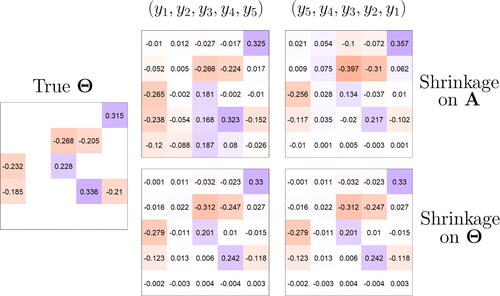
This simple example suggests that the estimates $\widehat{\mathbf{\Theta }}={\widehat{\mathbf{L}}}^{-1}\widehat{\mathbf{A}}$ diverge from the true $\mathbf{\Theta }$ and are sensitive to variable permutation. Instead, inference based on (2a) provides a more accurate identification of $\mathbf{\Theta }$, less sensitive to variable permutation.

3 Variational Bayes Inference

A variational approach to Bayesian inference requires to minimize the Kullback-Leibler ($KL$) divergence between an approximating density $q(\mathit{\xi })$ and the true posterior density $p(\mathit{\xi }|\mathbf{y})$, where $\mathit{\xi }$ denotes the set of parameters of interest. Ormerod and Wand (2010) show that minimizing the $KL$ divergence can be equivalently stated as the maximization of the “effective lower bound” (ELBO) denoted by $\underset{¯}{p}(\mathbf{y};q)$: (4) $$\begin{array}{c}{q}^{*}(\mathit{\xi })=\arg \underset{{}_{q(\mathit{\xi })\in \mathcal{Q}}}{\max }\hspace{0.17em}\log \hspace{0.17em}\underset{¯}{p}\left(\mathbf{y};q\right),\\ \underset{¯}{p}\left(\mathbf{y};q\right)=\int q(\mathit{\xi })\hspace{0.17em}\log \hspace{0.17em}\left\{\frac{p(\mathbf{y},\mathit{\xi })}{q(\mathit{\xi })}\right\} d\mathit{\xi },\end{array}$$(4) where $q^{*}(\mathit{\xi })\in \mathcal{Q}$ represents the optimal variational density and $\mathcal{Q}$ is a space of density functions. Depending on the assumption on $\mathcal{Q}$, one falls into different variational paradigms. For instance, given a partition of the parameters vector $\mathit{\xi }=\{{\mathit{\xi }}_1,\dots ,{\mathit{\xi }}_p\}$, a mean-field variational Bayes (MFVB) approach assumes a factorization of the form $q(\mathit{\xi })={\prod }_{j=1}^p{q}_i({\mathit{\xi }}_j)$. A closed-form expression for each optimal variational density $q^{\ast }({\mathit{\xi }}_j)$ can be defined as (5) $$\begin{array}{c}{q}^{\ast }({\mathit{\xi }}_j)\propto \hspace{0.17em}\exp \hspace{0.17em}\left\{{\mathbb{E}}_{q^{\star }(\mathit{\xi }\setminus {\mathit{\xi }}_j)}[\log \hspace{0.17em}p(\mathbf{y},\mathit{\xi })]\right\},\\ q^{\star }(\mathit{\xi }\setminus {\mathit{\xi }}_j)=\prod _{\stackrel{i=1}{i\ne j}}^p{q}_i({\mathit{\xi }}_i),\end{array}$$(5) where the expectation is taken with respect to the joint approximating density with the jth element of the partition removed $q^{\star }(\mathit{\xi }\setminus {\mathit{\xi }}_j)$. This allows the implementation of an efficient iterative algorithm to estimate the optimal density $q^{*}(\mathit{\xi })$. However, some components $q^{*}({\mathit{\xi }}_j)$ may remain too complex to handle and further restrictions are needed. If we assume that $q^{*}({\mathit{\xi }}_j)$ belongs to a pre-specified parametric family of distributions, the MFVB outlined above is sometimes labeled as semi-parametric (see Rohde and Wand 2016).

3.1 Optimal Variational Densities

We present a factorization of the variational density $q(\mathit{\xi })$ for the model in (2a). As a baseline, we consider a non-informative Normal prior for each entry of $\mathbf{\Theta }$; that is, ${\vartheta }_{j,k}\sim \mathrm{N}(0,\upsilon )$, for $j=1,\dots ,d$ and $k=1,\dots ,d+p+1$. In addition, let ${\psi }_j\sim \text{InvGa}(a_{\psi },b_{\psi })$ for $j=1,\dots ,d$, and ${\beta }_{j,k}\sim \mathrm{N}(0,\tau )$, for $j=2,\dots ,d$ and $k=1,\dots ,j-1$. Here, $\text{InvGa}(·,·)$ denotes the Inverse-Gamma distribution, and $a_{\psi }>0,b_{\psi }>0,\tau \gg 0$ and $\upsilon \gg 0$ are the related hyper-parameters.

Let $\mathit{\xi }={({\mathit{\vartheta }}^{⊺},{\mathbf{h}}^{⊺},{\mathit{\psi }}^{⊺},{\mathit{\beta }}^{⊺})}^{⊺}$ be the set of parameters of interest, the corresponding variational density can be factorized as $q(\mathit{\xi })=q(\mathit{\vartheta })q(\mathbf{h})q(\mathit{\psi })q(\mathit{\beta })$, where: (6) $$\begin{array}{c}q(\mathit{\vartheta })=\prod _{j=1}^{d}q({\mathit{\vartheta }}_j),\hspace{1em}q(\mathbf{h})=\prod _{j=1}^{d}q({\mathbf{h}}_j),\\ q(\mathit{\psi })=\prod _{j=1}^{d}q({\psi }_j),\hspace{1em}q(\mathit{\beta })=\prod _{j=2}^{d}q({\mathit{\beta }}_j).\end{array}$$(6)

For ease of exposition, we summarize in the main text the optimal variatonal density for the main parameters of interest $\mathbf{\Theta }$ for the baseline non-informative prior and three alternative hierarchical shrinkage priors. The full derivations of the optimal variational densities $q^{*}({\mathbf{h}}_j)\equiv {\mathrm{N}}_{T+1}({\mathit{\mu }}_{q(h_j)},{\mathbf{\Sigma }}_{q(h_j)}),q^{*}({\psi }_j)\equiv \text{InvGa}(a_{q({\psi }_j)},b_{q({\psi }_j)})$, and $q^{*}({\mathit{\beta }}_j)\equiv {\mathrm{N}}_{j-1}({\mathit{\mu }}_{q({\beta }_j)},{\mathbf{\Sigma }}_{q({\beta }_j)})$ are reported in Appendix B as Proposition B.1.1, B.1.7, and B.1.4, respectively. We leave to Proposition B.1.3 in Appendix B the derivations for the constant volatility case with ${\nu }_{j,t}={\nu }_j$ and ${\nu }_j\sim \text{Ga}(a_{\nu },b_{\nu })$ for $j=1,\dots ,d$, where $\text{Ga}(·,·)$ denotes the gamma distribution, and $a_{\nu }>0,b_{\nu }>0$. Appendix B also provides the analytical form of the lower bound for each set of parameters.

Proposition 3.1 provides the optimal variational density for the jth row of $\mathbf{\Theta }$ under the Normal prior specification ${\vartheta }_{j,k}\sim \mathrm{N}(0,\upsilon )$. The proof and analytical derivations are reported in Appendix B.1.

Proposition 3.1.

The optimal variational density for ${\mathit{\vartheta }}_j$ is $q^{*}({\mathit{\vartheta }}_j)\equiv {\mathrm{N}}_{d+p+1}({\mathit{\mu }}_{q({\vartheta }_j)},{\mathbf{\Sigma }}_{q({\vartheta }_j)})$ with hyper-parameters: (7) $$\begin{array}{c}{\mathbf{\Sigma }}_{q({\vartheta }_j)}={\left(\sum _{t=1}^T{\mathit{\mu }}_{q({\omega }_{j,j,t})}{\mathbf{z}}_{t-1}{\mathbf{z}}_{t-1}^{⊺}+1/\upsilon {\mathbf{I}}_{d+p+1}\right)}^{-1},\\ {\mathit{\mu }}_{q({\vartheta }_j)}={\mathbf{\Sigma }}_{q({\vartheta }_j)}(\sum _{t=1}^T\left({\mathit{\mu }}_{q({\mathbf{\omega }}_{j,t})}\otimes {\mathbf{z}}_{t-1}\right){\mathbf{y}}_t\\ -\sum _{t=1}^T\left({\mathit{\mu }}_{q({\mathbf{\omega }}_{j,-j,t})}\otimes {\mathbf{z}}_{t-1}{\mathbf{z}}_{t-1}^{⊺}\right){\mathit{\mu }}_{q({\vartheta }_{-j})}),\end{array}$$(7) where $\mathit{\vartheta }=(\begin{array}{c}{\mathit{\vartheta }}_j\\ {\mathit{\vartheta }}_{-j}\end{array})$ and ${\mathit{\omega }}_{j,t}$ denotes the jth row of ${\mathbf{\Omega }}_t=(\begin{array}{cc}{\omega }_{j,j,t}& {\mathit{\omega }}_{j,-j,t}\\ {\mathit{\omega }}_{-j,j,t}& {\mathbf{\Omega }}_{-j,-j,t}\end{array}).$

Note that although the multivariate model is reduced to a sequence of univariate regressions, the analytical form of the variational means ${\mathit{\mu }}_{q({\vartheta }_j)}$ in Proposition 3.1 depends on all the other rows through ${\mathit{\mu }}_{q({\vartheta }_{-j})}$. As a result, the estimates of ${\vartheta }_j$ explicitly depend on all of the other ${\vartheta }_{-j}$. This addresses the issue in the MCMC algorithm of Carriero, Clark, and Marcellino (2019), which has been highlighted by Bognanni (2022) and corrected by Carriero et al. (2022).

Bayesian adaptive-Lasso

The Bayesian adaptive-Lasso of Leng, Tran, and Nott (2014) extends the original work of Park and Casella (2008) by assuming a different shrinkage for each regression parameter based on a Laplace distribution with an individual scaling parameter ${\vartheta }_{j,k}|{\lambda }_{j,k}\sim \text{Lap}({\lambda }_{j,k})$, for $j=1,\dots ,d$ and $k=1,\dots ,d+p+1$. The latter can be represented as a scale mixture of Normal distributions with an exponential mixing density, ${\vartheta }_{j,k}|{\upsilon }_{j,k}\sim \mathrm{N}(0,{\upsilon }_{j,k}),{\upsilon }_{j,k}|{\lambda }_{j,k}^2\sim \hspace{0.17em}\mathrm{Exp}\hspace{0.17em}({\lambda }_{j,k}^2/2)$. The scaling parameters ${\lambda }_{j,k}^2$ are not fixed but are inferred from the data by assuming a common hyper-prior distribution ${\lambda }_{j,k}^2\sim \text{Ga}(h_1,h_2)$, where $h_1,h_2>0$.

Let ${\mathit{\xi }}_{\mathrm{L}}=({\mathit{\xi }}^{⊺},{\mathit{\upsilon }}^{⊺},{({\mathit{\lambda }}^2)}^{⊺}){)}^{⊺}$ be the vector $\mathit{\xi }$ augmented with the adaptive-Lasso prior parameters. The distribution $q({\mathit{\xi }}_{\mathrm{L}})$ can be factorized as, (8) $$\begin{array}{c}q({\mathit{\xi }}_{\mathrm{L}})=q(\mathit{\xi })q(\mathit{\upsilon },{\mathit{\lambda }}^2),\\ q(\mathit{\upsilon },{\mathit{\lambda }}^2)=\prod _{j=1}^d\prod _{k=1}^{d+p+1}q({\upsilon }_{j,k})q({\lambda }_{j,k}^2),\end{array}$$(8)

Proposition 3.2 provides the optimal variational density for the jth row of $\mathbf{\Theta }$ under the Bayesian adaptive-Lasso prior specification ${\vartheta }_{j,k}|{\upsilon }_{j,k}\sim \mathrm{N}(0,{\upsilon }_{j,k}),{\upsilon }_{j,k}|{\lambda }_{j,k}^2\sim \hspace{0.17em}\mathrm{Exp}\hspace{0.17em}({\lambda }_{j,k}^2/2)$, and ${\lambda }_{j,k}^2\sim \text{Ga}(h_1,h_2)$. The proof and the analytical derivations are reported in Appendix B.2.

Proposition 3.2.

The optimal variational density for ${\mathit{\vartheta }}_j$ is $q^{*}({\mathit{\vartheta }}_j)\equiv {\mathrm{N}}_{d+p+1}({\mathit{\mu }}_{q({\vartheta }_j)},{\mathbf{\Sigma }}_{q({\vartheta }_j)})$ with ${\mathbf{\Sigma }}_{q({\vartheta }_j)}=({\sum }_{t=1}^T{\mathit{\mu }}_{q({\omega }_{j,j,t})}$ ${{\mathbf{z}}_{t-1}{\mathbf{z}}_{t-1}^{⊺}+\text{Diag}({\mathit{\mu }}_{q(1/{\mathbf{\upsilon }}_j)}))}^{-1}$, where $\text{Diag}({\mathit{\mu }}_{q(1/{\mathbf{\upsilon }}_j)})$ is a diagonal matrix with elements ${\mathit{\mu }}_{q(1/{\mathbf{\upsilon }}_j)}=({\mu }_{q(1/{\upsilon }_{j,1})},{\mu }_{q(1/{\upsilon }_{j,2})},\dots ,$ ${\mu }_{q(1/{\upsilon }_{j,d+p+1})})$. The parameters ${\mathit{\mu }}_{q({\vartheta }_j)}$ and ${\mathit{\mu }}_{q({\omega }_{j,j,t})}$ are as in Proposition 3.1. The optimal variational densities of the scaling parameters are $q^{*}({\lambda }_{j,k}^2)\equiv \text{Ga}(a_{q({\lambda }_{j,k}^2)},b_{q({\lambda }_{j,k}^2)})$ with $a_{q({\lambda }_{j,k}^2)},b_{q({\lambda }_{j,k}^2)}$ defined in (B.20), and $q^{*}(1/{\upsilon }_{j,k})\equiv \text{IG}(a_{q(1/{\upsilon }_{j,k})},b_{q(1/{\upsilon }_{j,k})})$ with $a_{q({\upsilon }_{j,k})},b_{q({\upsilon }_{j,k})}$ defined in (B.19).

Adaptive Normal-Gamma

We expand the original Normal-Gamma prior in Griffin and Brown (2010) by assuming that each regression coefficient has a different shrinkage parameter. The hierarchical specification requires that ${\vartheta }_{j,k}|{\upsilon }_{j,k}\sim \mathrm{N}(0,{\upsilon }_{j,k})$, and ${\upsilon }_{j,k}|{\eta }_j,{\lambda }_{j,k}\sim \text{Ga}({\eta }_j,{\eta }_j{\lambda }_{j,k}/2)$ for $j=1,\dots ,d$ and $k=1,\dots ,d+p+1$. Note that by restricting ${\eta }_j=1$ one obtains the adaptive-Lasso prior. The marginalization over the variance ${\upsilon }_{j,k}$ leads to $p({\vartheta }_{j,k}|{\eta }_j,{\lambda }_{j,k})$ which corresponds to a Variance-Gamma distribution. The hyper-parameters η_j and ${\lambda }_{j,k}$ are not fixed but are inferred from the data by assuming two common hyper-priors ${\lambda }_{j,k}\sim \text{Ga}(h_1,h_2)$ and ${\eta }_j\sim \hspace{0.17em}\mathrm{Exp}\hspace{0.17em}(h_3)$, where $h_l>0$ for l = 1, 2, 3.

Let ${\mathit{\xi }}_{\text{NG}}={({\mathit{\xi }}^{⊺},{\mathit{\upsilon }}^{⊺},{\mathit{\lambda }}^{⊺},{\mathit{\eta }}^{⊺})}^{⊺}$ be the vector $\mathit{\xi }$ augmented with the parameters of the adaptive Normal-Gamma prior. The joint distribution $q({\mathit{\xi }}_{\text{NG}})$ can be factorized as, (9) $$\begin{array}{c}q({\mathit{\xi }}_{\text{NG}})=q(\mathit{\xi })q(\mathit{\upsilon },\mathit{\lambda },\mathit{\eta }),\\ q(\mathit{\upsilon },\mathit{\lambda },\mathit{\eta })=\prod _{j=1}^{d}q({\eta }_j)\prod _{k=1}^{d+p+1}q({\upsilon }_{j,k})q({\lambda }_{j,k}).\end{array}$$(9)

Proposition 3.3 provides the optimal variational density for the jth row of $\mathbf{\Theta }$ under an adaptive Normal-Gamma specification ${\upsilon }_{j,k}|{\eta }_j,{\lambda }_{j,k}\sim \text{Ga}({\eta }_j,{\eta }_j{\lambda }_{j,k}/2),{\lambda }_{j,k}\sim \text{Ga}(h_1,h_2)$ and ${\eta }_j\sim \hspace{0.17em}\mathrm{Exp}\hspace{0.17em}(h_3)$. The proof and analytical derivations are reported in Appendix B.3.

Proposition 3.3.

The optimal variational density for ${\mathit{\vartheta }}_j$ is $q^{*}({\mathit{\vartheta }}_j)\equiv {\mathrm{N}}_{d+p+1}({\mathit{\mu }}_{q({\vartheta }_j)},{\mathbf{\Sigma }}_{q({\vartheta }_j)})$ with ${\mathbf{\Sigma }}_{q({\vartheta }_j)}=({\sum }_{t=1}^T{\mathit{\mu }}_{q({\omega }_{j,j,t})}$ ${{\mathbf{z}}_{t-1}{\mathbf{z}}_{t-1}^{⊺}+\text{Diag}({\mathit{\mu }}_{q(1/{\mathbf{\upsilon }}_j)}))}^{-1}$, where $\text{Diag}({\mathit{\mu }}_{q(1/{\mathbf{\upsilon }}_j)})$ is a diagonal matrix with elements ${\mathit{\mu }}_{q(1/{\mathbf{\upsilon }}_j)}=({\mu }_{q(1/{\upsilon }_{j,1})},{\mu }_{q(1/{\upsilon }_{j,2})},\dots ,$ ${\mu }_{q(1/{\upsilon }_{j,d+p+1})})$. The parameters ${\mathit{\mu }}_{q({\vartheta }_j)}$ and ${\mathit{\mu }}_{q({\omega }_{j,j,t})}$ are as in Proposition 3.1. The optimal variational densities of the scaling parameters are $q^{*}({\lambda }_{j,k})\equiv \text{Ga}(a_{q({\lambda }_{j,k})},b_{q({\lambda }_{j,k})})$ with $a_{q({\lambda }_{j,k})},b_{q({\lambda }_{j,k})}$ defined in (B.24), and $q^{*}({\upsilon }_{j,k})\equiv \text{GIG}({\zeta }_{q({\upsilon }_{j,k})},a_{q({\upsilon }_{j,k})},b_{q({\upsilon }_{j,k})})$ is a generalized inverse normal distribution with ${\zeta }_{q({\upsilon }_{j,k})},a_{q({\upsilon }_{j,k})},$ $b_{q({\upsilon }_{j,k})}$ defined in (B.23).

The optimal density for the parameter η_j is not a known distribution function. Proposition B.3.3 in Appendix B.3 provides an analytical approximation of its moments so that the optimal density can be calculated via numerical integration.

Horseshoe prior

We consider the Horseshoe prior as proposed by Carvalho, Polson, and Scott (2009, 2010). This is based on the hierarchical specification ${\vartheta }_{j,k}|{\upsilon }_{j,k}^2,{\gamma }^2\sim \mathrm{N}(0,{\gamma }^2{\upsilon }_{j,k}^2),\gamma \sim {\mathsf{C}}^{+}(0,1),{\upsilon }_{j,k}\sim {\mathsf{C}}^{+}(0,1)$, where ${\mathsf{C}}^{+}(0,1)$ denotes the standard half-Cauchy distribution with probability density function equal to $f(x)=2/\{\pi (1+x^2)\}{⊮}_{(0,\infty )}(x)$. The Horseshoe is a global-local prior that implies an aggressive shrinkage of weak signals without affecting the strong ones (see, e.g., Polson and Scott 2011). We follow Wand et al. (2011) and leverage on a scale mixture representation of the half-Cauchy distribution as, (10) $$\begin{array}{c}{\vartheta }_{j,k}|{\upsilon }_{j,k}^2,{\gamma }^2\sim \mathrm{N}(0,{\gamma }^2{\upsilon }_{j,k}^2),\hspace{1em}{\gamma }^2|\eta \sim \text{InvGa}(1/2,1/\eta ),\\ {\upsilon }_{j,k}^2|{\lambda }_{j,k}\sim \text{InvGa}(1/2,1/{\lambda }_{j,k}),\\ \eta \sim \text{InvGa}(1/2,1),\\ {\lambda }_{j,k}\sim \text{InvGa}(1/2,1),\end{array}$$(10) where the local and global shrinkage parameters are ${\upsilon }_{j,k}^2$ and ${\gamma }^2$, respectively.

Let ${\mathit{\xi }}_{\text{HS}}={({\mathit{\xi }}^{⊺},{({\mathit{\upsilon }}^2)}^{⊺},{\gamma }^2,{\mathit{\lambda }}^{⊺},\eta )}^{⊺}$ be the vector $\mathit{\xi }$ augmented with the parameters of the Horseshoe prior. The joint distribution ${\mathit{\xi }}_{\text{HS}}$ can be factorized as, (11) $$\begin{array}{c}q({\mathit{\xi }}_{\text{HS}})=q(\mathit{\xi })q({\mathit{\upsilon }}^2,{\gamma }^2,\mathit{\lambda },\eta ),\\ q({\mathit{\upsilon }}^2,{\gamma }^2,\mathit{\lambda },\eta )=q({\gamma }^2)q(\eta )\prod _{j=1}^d\prod _{k=1}^{d+p+1}q({\upsilon }_{j,k}^2)q({\lambda }_{j,k}).\end{array}$$(11)

Proposition 3.4 provides the optimal variational density for the jth row of $\mathbf{\Theta }$ under the Horseshoe prior outlined in (10). The proof and analytical derivations are reported in Appendix B.4.

Proposition 3.4.

The optimal variational density for ${\mathit{\vartheta }}_j$ is $q^{*}({\mathit{\vartheta }}_j)\equiv {\mathrm{N}}_{d+p+1}({\mathit{\mu }}_{q({\vartheta }_j)},{\mathbf{\Sigma }}_{q({\vartheta }_j)})$ with ${\mathbf{\Sigma }}_{q({\vartheta }_j)}=({\sum }_{t=1}^T{\mathit{\mu }}_{q({\omega }_{j,j,t})}$ ${{\mathbf{z}}_{t-1}{\mathbf{z}}_{t-1}^{⊺}+{\mu }_{q(1/{\gamma }^2)}\text{Diag}({\mathit{\mu }}_{q(1/{\mathbf{\upsilon }}_j^2)}))}^{-1}$, where $\text{Diag}({\mathit{\mu }}_{q(1/{\mathbf{\upsilon }}_j^2)})$ is a diagonal matrix with elements ${\mathit{\mu }}_{q(1/{\mathbf{\upsilon }}_j^2)}=({\mu }_{q(1/{\upsilon }_{j,1}^2)},$ ${\mu }_{q(1/{\upsilon }_{j,2}^2)},\dots ,{\mu }_{q(1/{\upsilon }_{j,d+p+1}^2)})$. The parameters ${\mathit{\mu }}_{q({\vartheta }_j)}$ and ${\mathit{\mu }}_{q({\omega }_{j,j,t})}$ are as in Proposition 3.1. The optimal variational densities for the global shrinkage is $q^{*}({\gamma }^2)\equiv \text{InvGa}(\frac{1}{2}\{d(d+p+1)+1\},$ $b_{q({\gamma }^2)})$ with $b_{q({\gamma }^2)}$ defined in (B.33), and $q^{*}(\eta )\equiv \text{InvGa}$ $(1,b_{q(\eta )})$ with $b_{q(\eta )}$ defined in (B.35). The optimal variational densities for the local shrinkage parameters are $q^{*}({\upsilon }_{j,k}^2)\equiv \text{InvGa}(1,b_{q({\upsilon }_{j,k}^2)})$ and $q^{*}({\lambda }_{j,k})\equiv \text{InvGa}(1,b_{q({\lambda }_{j,k})})$, with $b_{q({\upsilon }_{j,k}^2)}$ and $b_{q({\lambda }_{j,k})}$ defined in (B.32) and (B.34), respectively.

3.2 From Shrinkage to Sparsity

In addition to computational tractability, shrinking rather than selecting is a defining feature of the hierarchical priors outlined in Section 3.1. Yet, posterior estimates of $\mathbf{\Theta }$ are non-sparse and thus can not provide exact differentiation between significant versus nonsignificant predictors. The latter is particularly relevant since we ultimately want to assess the accuracy of our variational inference approach—versus existing MCMC and variational Bayes algorithms—in identifying the exact structure of $\mathbf{\Theta }$.

To address this issue, we build upon Ray and Bhattacharya (2018) and implement a Signal Adaptive Variable Selector (SAVS) algorithm to induce sparsity in $\widehat{\mathbf{\Theta }}$, conditional on a given prior. The SAVS is a post-processing algorithm which divides signals and nulls on the basis of the point estimates of the regression coefficients (see, e.g., Hauzenberger, Huber, and Onorante 2021). Specifically, let ${\widehat{\vartheta }}_j$ be the posterior estimate of ${\vartheta }_j$ and ${\mathbf{z}}_j$ be the associated vector of covariates. If $\left|{\widehat{\vartheta }}_j\right| \left|\right|{\mathbf{z}}_j|{|}^2\le |{\widehat{\vartheta }}_j{|}^{-2}$ we set ${\widehat{\vartheta }}_j=0$, where $\left|\right|·\left|\right|$ denotes the Euclidean norm.

The reason why we rely on the SAVS post-processing to induce sparsity in the posterior estimates is threefold. First, as highlighted by Ray and Bhattacharya (2018), the SAVS represents an automatic procedure in which the sparsity-inducing property directly depends on the effectiveness of the shrinkage performed on ${\widehat{\vartheta }}_j$. This refers to the precision of the posterior mean estimates; that is, the more accurate is ${\widehat{\vartheta }}_j$, the more precise is the identification of the nonzero elements in $\mathbf{\Theta }$. Second, the SAVS is “agnostic” with respect to the shrinkage prior or estimation approach adopted, so it represents a natural tool to compare different estimation methods. Third, it is decision-theoretically motivated as it grounds on the idea of minimizing the posterior expected loss (see, e.g., Huber, Koop, and Onorante 2021).

In addition to SAVS, we expand on Hahn and Carvalho (2015) and provide a multivariate extension to their least-angle regression originally built for univariate regressions. Appendix D.2 provides the full derivation as well as a complete discussion of the drawbacks compared to SAVS. In addition, Appendix D.2 reports the results of a direct comparison between the SAVS and our multivariate extension to Hahn and Carvalho (2015) based on simulated data.

3.3 Variational Predictive Density

Consider the posterior distribution $p(\mathit{\xi }|{\mathbf{z}}_{1:t})$ given the information set ${\mathbf{z}}_{1:t}=\left\{{\mathbf{y}}_{1:t},{\mathbf{x}}_{1:t}\right\}$ and the conditional likelihood $p({\mathbf{y}}_{t+1}|{\mathbf{z}}_t,\mathit{\xi })$. A standard predictive density takes the form, (12) $$p({\mathbf{y}}_{t+1}|{\mathbf{z}}_{1:t})=\int p({\mathbf{y}}_{t+1}|{\mathbf{z}}_t,\mathit{\xi })p(\mathit{\xi }|{\mathbf{z}}_{1:t})d\mathit{\xi }.$$(12)

Given an optimal variational density $q^{*}(\mathit{\xi })$ that approximates $p(\mathit{\xi }|{\mathbf{z}}_{1:t})$, we follow Gunawan, Kohn, and Nott (2020) and obtain the variational predictive distribution (13) $$\begin{array}{c}q({\mathbf{y}}_{t+1}|{\mathbf{z}}_{1:t})=\int p({\mathbf{y}}_{t+1}|{\mathbf{z}}_t,\mathit{\xi })q^{*}(\mathit{\xi })d\mathit{\xi }\\ =\iint p({\mathbf{y}}_{t+1}|{\mathbf{z}}_t,\mathit{\vartheta },{\mathbf{\Omega }}_t)q^{*}(\mathit{\vartheta })q^{*}({\mathbf{\Omega }}_t)d\mathit{\vartheta } d{\mathbf{\Omega }}_t.\mathrm{\hspace{1em}}\mathrm{\hspace{1em}}\end{array}$$(13)

Although an analytical expression for (13) is not available, a simulation-based estimator for $q({\mathbf{y}}_{t+1}|{\mathbf{z}}_{1:t})$ can be obtained through Monte Carlo integration by averaging $p({\mathbf{y}}_{t+1}|{\mathbf{z}}_t,{\mathit{\xi }}^{(i)})$ over the draws ${\mathit{\xi }}^{(i)}\sim q^{\ast }(\mathit{\xi })$, such that $\widehat{q}({\mathbf{y}}_{t+1}|{\mathbf{z}}_{1:t})=N^{-1}{\sum }_{i=1}^{N}p({\mathbf{y}}_{t+1}|{\mathbf{z}}_t,{\mathit{\xi }}^{(i)})$. Note that a complete characterization of the optimal variational predictive density entails $q^{*}({\mathbf{\Omega }}_t)$ with ${\mathbf{\Omega }}_t={\mathbf{L}}^{⊺}{\mathbf{V}}_t\mathbf{L}$. Proposition 3.5 shows that conditional on L and ${\mathbf{V}}_t$, the optimal distribution of ${\mathbf{\Omega }}_t$ can be approximated by a d-dimensional Wishart distribution ${\text{Wishart}}_d({\delta }_t,{\mathbf{H}}_t)$, where δ_t and ${\mathbf{H}}_t$ are the degrees of freedom parameter and the scaling matrix, respectively.

Proposition 3.5.

The approximate distribution $\tilde{q}$ of ${\mathbf{\Omega }}_t$ is ${\text{Wishart}}_d({\widehat{\delta }}_t,{\widehat{\mathbf{H}}}_t)$, where the scaling matrix is given by ${\widehat{\mathbf{H}}}_t={\widehat{\delta }}_t^{-1}{\mathbb{E}}_q\left[{\mathbf{\Omega }}_t\right]$ and ${\widehat{\delta }}_t$ can be obtained numerically as the solution of a convex optimization problem.

The complete proof is available in Appendix C.1 and is based on the Expectation Propagation (EP) approach proposed by Minka (2001). In order to implement this approach, there is no need to know $q^{*}({\mathbf{\Omega }}_t)$, but it is sufficient to be able to compute ${\mathbb{E}}_q({\mathbf{\Omega }}_t)$. The latter can be reconstructed based on the optimal variational densities of the Cholesky factor $q^{*}(\mathit{\beta })$–and therefore for L–and of $q^{*}({\mathbf{V}}_t)$. The simulation results in Appendix C.1 show that the proposed Wishart distribution provides an accurate approximation of $q^{*}({\mathbf{\Omega }}_t)$ for both small and large dimensional models.

Based on Proposition 3.5, we can further simplify (13) by integrating ${\mathbf{\Omega }}_t$ such that (14) $$q({\mathbf{y}}_{t+1}|{\mathbf{z}}_{1:t})=\int h({\mathbf{y}}_{t+1}|{\mathbf{z}}_t,\mathit{\vartheta })q^{*}(\mathit{\vartheta })d\mathit{\vartheta },$$(14) where $h({\mathbf{y}}_{t+1}|{\mathbf{z}}_t,\mathit{\vartheta })$ denotes the probability density function of a multivariate Student-t distribution ${\mathsf{t}}_v(\mathbf{m},\mathbf{S})$ with mean $\mathbf{m}=\mathbf{\Theta }{\mathbf{z}}_t$, scaling matrix $\mathbf{S}={(v\widehat{\mathbf{H}})}^{-1}$, and degrees of freedom parameter $v=\widehat{\delta }-d+1$. As a result, the predictive distribution can be more efficiently approximated by averaging the density of the multivariate Student-t $h({\mathbf{y}}_{t+1}|{\mathbf{z}}_t,{\mathit{\vartheta }}^{(i)})$ over the draws ${\mathit{\vartheta }}^{(i)}\sim q^{\ast }(\mathit{\vartheta })$, for $i=1,\dots ,N$, such that $\widehat{q}({\mathbf{y}}_{t+1}|{\mathbf{z}}_{1:t})=N^{-1}{\sum }_{i=1}^{N}h({\mathbf{y}}_{t+1}|{\mathbf{z}}_t,{\mathit{\vartheta }}^{(i)})$.

Note that the main advantage of the approximation obtained from Proposition 3.5 is to allow for a considerably faster computation of the variational predictive density, compared to using $q^{*}(\mathbf{L})$ and $q^{*}({\mathbf{V}}_t)$ as stationary distributions to sample ${\mathbf{\Omega }}_t$, similar to an MCMC. This is because the scaling matrix of the Wishart distribution is available in closed form, and the computation of degrees of freedom requires only a one-dimensional optimization. In Appendix C.2, we discuss a further simplification that minimizes the KL divergence between the multivariate Student-t and a multivariate Normal distribution.

4 Simulation Study

In this section, we report the results of an extensive simulation study designed to compare the properties of our estimation approach against both MCMC and variational Bayes methods for large VAR models. To begin, we compare our VB algorithm against the MCMC approach of Chan and Eisenstat (2018) and Cross, Hou, and Poon (2020) and the variational inference algorithm proposed by Chan and Yu (2022) and Gefang, Koop, and Poon (2023). Both approaches are built upon the structural VAR representation in (2b). In addition, we also compare our VB method against the MCMC approach developed by Huber and Feldkircher (2019) and Gruber and Kastner (2022), which is based upon a nonlinear parameterization as in (2a).

For comparability with Gruber and Kastner (2022) and Gefang, Koop, and Poon (2023), which do not consider the presence of exogenous predictors, we consider a standard VAR(1) as a data generating process. Consistent with the empirical implementations, we set T = 360 and d = 30, 49. The choice of d is due to the two alternative industry classifications explored in the main empirical analysis. We assume either a moderate—50% of zeros—or a high—90% of zeros—level of sparsity in the true matrix $\mathbf{\Theta }$. The latter is generated as follows: we fix to zero $s·d^2$ entries at random, with $s=0.5,0.9$ and d = 30, 49, and the remaining nonzero coefficients are sampled from a mixture of two normal distributions with means equal to ±0.08 and standard deviation 0.1. Appendix D provides additional details on the data-generating process and additional simulation results for d = 15.

4.1 Estimation Accuracy

As a measure of point estimation accuracy, we first look at the Frobenius norm $\left|\right|\mathbf{\Theta }-\widehat{\mathbf{\Theta }}{\Vert }_F$. The latter measures the difference between the true $\mathbf{\Theta }$ observed at each simulation and its estimate $\widehat{\mathbf{\Theta }}$. In addition, we compare the ability of each estimation method to identify the nonzero elements in the true $\mathbf{\Theta }$ based on the F1 score. This is expressed as a function of counts of true positives (tp), false positives (fp) and false negatives (fn), $$\mathrm{F}1=\frac{2tp}{2tp+fp+fn}.$$

The F1 score takes value one if identification is perfect, that is, no false positives and no false negatives, and zero if there are no true positives. We compute both measures of estimation accuracy on N = 100 replications and compare each estimation method and prior specification. The estimates from the MCMC specifications are based on 5000 posterior simulations after discarding the first 5000 as a burn-in sample.

Point estimates

Figure 2 shows the box charts summarizing the Frobenius norm $\left|\right|\mathbf{\Theta }-\widehat{\mathbf{\Theta }}{\Vert }_F$ across N = 100 replications. We label the linearized MCMC and variational methods with LMCMC and LVB, respectively, with MCMC the nonlinear method of Gruber and Kastner (2022) and with VB our variational inference method. To increase readability, we separate the results by prior and color-coding the four estimation methods. For instance, for a given subplot, we report the results for the Normal, adaptive-Lasso, adaptive Normal-Gamma and Horseshoe priors from the left to the right panel. Within each panel, the simulation results for the LMCMC, LVB, MCMC, and VB estimates are reported in red, yellow, light blue, and green, respectively.

Fig. 2 Frobenius norm of $\mathbf{\Theta }-\widehat{\mathbf{\Theta }}$ across N = 100 replications, for different shrinkage priors and different inference methods.

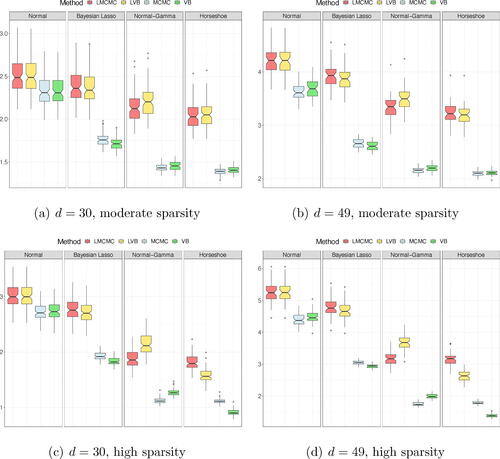
Beginning with the moderate sparsity case (top panels), the simulation results show that LMCMC and LVB approaches tend to perform equally across different shrinkage priors, with the only exception of the Normal-Gamma prior, whereby LMCMC slightly outperforms LVB. However, the discrepancy between the two structural VAR representation methods increases when sparsity becomes more pervasive (see bottom panels).

Overall, the simulation results support our view that by eliciting shrinkage priors directly on $\mathbf{\Theta }$—as per the parameterization in (2a)—the accuracy of the posterior estimates improves. The mean squared errors obtained from MCMC and VB are lower compared to both LMCMC and LVB. This holds for all priors and model dimensions. The accuracy with d = 30 of the MCMC and VB is virtually the same. Yet, with d = 49, our VB is slightly more accurate than MCMC for the adaptive-Lasso and the Horseshoe prior.

Sparsity identification

Figure 3 shows the box charts of F1 scores across N = 100 simulations. The labeling is the same as in Figure 2. Both LMCMC and LVB produce a rather dismal identification of the nonzero elements in $\mathbf{\Theta }$ across prior and model dimensions. This is due to the fact that $\widehat{\mathbf{\Theta }}={\widehat{\mathbf{L}}}^{-1}\widehat{\mathbf{A}}$ in (2b) so that a sparse $\widehat{\mathbf{A}}$ does not translate into a sparse $\widehat{\mathbf{\Theta }}$, and thus is less accurate in identifying the nonzero coefficients in the true $\mathbf{\Theta }$. When the level of sparsity increases, so does the divergence between A and $\mathbf{\Theta }$.

Fig. 3 F1 score computed across N = 100 replications by looking at the true non-null parameters in $\mathbf{\Theta }$ and the non-null parameters estimated based on $\widehat{\mathbf{\Theta }}$.

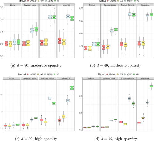
Consistent with our argument in favor of the parameterization in (2a), both the MCMC and VB approaches produce a more accurate identification of the nonzero coefficients in $\mathbf{\Theta }$, as shown by the F1 score. The gap between LMCMC, LVB, versus MCMC and VB becomes larger for higher levels of sparsity. This result holds across different hierarchical shrinkage priors and for different model dimensions. Yet, our VB approach turns out to be more accurate than MCMC under the adaptive-Lasso and Horseshoe priors for higher sparsity levels.

Note that sparsity in the posterior estimates for $\widehat{\mathbf{\Theta }}$ for different hierarchical shrinkage priors is induced in the simulation results by using the SAVS algorithm of Ray and Bhattacharya (2018). Appendix D.2 provides additional simulation results obtained by implementing a multivariate version of the post-processing method proposed by Hahn and Carvalho (2015) as an alternative to the SAVS. The F1 scores are largely the same across methods; in fact, the evidence is even more in favor of our VB, compared to its MCMC counterpart when using the extended Hahn and Carvalho (2015) approach: our VB is more accurate than MCMC with a Normal-Gamma prior.

Computational efficiency

Figure 4 reports the computational time—expressed in a log-minute scale—required by each competing estimation approach under different shrinkage priors. To highlight the performance for a given prior, we separate the results by estimation methods and color-coding the four different shrinkage priors. For instance, for a given subplot, we report the results for the LMCMC, LVB, MCMC, and VB estimates from left to right panel. Within each panel, the Normal, adaptive-Lasso, adaptive Normal-Gamma, and Horseshoe priors are colored in shades of gray from light (left) to dark (right) gray, respectively. To guarantee more reliable comparability, we re-coded all competing methods in Rcpp and used the same 2.5 GHz Intel Xeon W-2175 with 32GB of RAM for all implementations. This allows us to compare all methods on an equal footing.

Fig. 4 Computational time required by each estimation approach for different hierarchical shrinkage priors. The time is expressed on a log-minute scale.

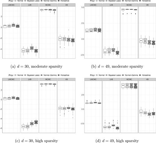
The results highlight that our VB approach has a clear computational advantage compared to linear and nonlinear MCMC methods. For instance, for d = 30, our VB is more than 100 times faster than the MCMC of Gruber and Kastner (2022) and more than 10 times faster than the LMCMC of Cross, Hou, and Poon (2020), respectively. The gap in favor of our VB method increases in larger dimensions; for d = 49, the MCMC approach takes on average almost 60 min to generate posterior estimates which are comparably accurate to our VB, which instead takes on average between 30–40 sec for the estimate. Such an efficiency gap has profound implications for a practical forecasting implementation, especially within the context of recursive predictions with higher frequency data such as stock returns (see Section 5.2). Perhaps not surprisingly, the LVB approach of Chan and Yu (2022) and Gefang, Koop, and Poon (2023) is highly competitive in terms of computational efficiency. However, being built on a structural VAR formulation, Figures 2 and 3 show that the computational efficiency of the LVB approach comes at the cost of substantially lower estimation accuracy.

Appendix E.1 provides a further qualitative discussion on the computational costs of some of the existing MCMC approaches. We review some of the results reported in the original papers and show that these largely align with our own findings. In addition, we also discuss some of the limitations of the nonlinear MCMC for the recursive forecasting implementation.

Robustness to variable permutation

At the paper’s outset, we argue that a conventional structural VAR formulation potentially generates posterior estimates sensitive to variable permutation. That is posterior estimates of $\mathbf{\Theta }$ depend on the ordering imposed on the target variables ${\mathbf{y}}_t$, conditional on a given prior. To highlight this issue, in Appendix D, we report additional simulation results for all estimation methods and shrinkage priors under variable permutation. The results show that the accuracy of the posterior estimates from both LMCMC and LVB changes once the variable’s ordering is reversed (see Figure D.4). This is especially evident for the Normal-Gamma and Horseshoe priors and when zero coefficients in $\mathbf{\Theta }$ are more pervasive. On the other hand, the estimation accuracy of both the MCMC approach of Gruber and Kastner (2022) and our VB method do not substantially deteriorate by arbitrarily changing the ordering of the target variables.

Note that although our approach provides estimates and point predictions that are robust with respect to variable ordering, density forecasts might differ. To address this issue, Arias, Rubio-Ramirez, and (2023) propose a time-varying correlation matrix model based on the parameterization of Archakov and Hansen (2021). Still, the latter is computationally intensive and may not be suitable for large datasets. As shown by Chan, Koop, and Yu (2023), a decomposition ${\mathbf{\Omega }}_t={\mathbf{L}}^{⊺}{\mathbf{V}}_t\mathbf{L}$, where L is an unrestricted square matrix rather than lower-triangular, represent a valid alternative toward permutation invariance in high-dimensional settings.

5 A Empirical Study of Industry Returns Predictability

We investigate both the statistical and economic value of our variational Bayes approach within the context of US industry returns predictability. To expand the scope of the empirical exercise, we consider two alternative industry aggregations: d = 30 industry portfolios from July 1926 to May 2020 and a larger cross-section of d = 49 industry portfolios from July 1969 to May 2020. The size of the cross sections changes due to a different industry classification. At the end of June in year t, each NYSE, AMEX, and NASDAQ stock is assigned to an industry portfolio based on its four-digit SIC code. Thus, the returns on a given value-weighted portfolio are computed from July of t to June of t + 1. The sample periods cover major events, from the great depression to the Covid-19 outbreak.

In addition to cross-industry portfolio returns, we consider a variety of predictors, such as the returns on the market portfolio (mkt), and the returns on four alternative long-short investment strategies based on market capitalization (smb), book-to-market ratios (hml), operating profitability (rmw) and firm investments (cma) (see Fama and French 2015). We also consider a set of additional macroeconomic predictors from Goyal and Welch (2008), such as the log price-dividend ratio (pd), the difference between the long term yield on government bonds and the T-bill (term), the BAA-AAA bond yields difference (credit), the monthly log change in the CPI (infl), the aggregate market book-to-market ratio (bm), the net-equity issuing activity (ntis) and the corporate bond returns (corpr).

5.1 In-Sample Parameter Estimates

In order to highlight some of the main properties of each method, we first report the in-sample estimates of $\mathbf{\Theta }$ for the d = 49 industry case for all priors. Figure 5 compares $\widehat{\mathbf{\Theta }}$ based on the full sample obtained from the LMCMC and the LVB with constant volatility, and our VB with and without stochastic volatility. Appendix E.3 reports the additional in-sample estimates for d = 30 industry portfolios.

Fig. 5 Variational Bayes estimates of the regression coefficients $\mathbf{\Theta }$ for different estimation methods. We report the estimates for the d = 49 industry case obtained for all priors. We report the results for VB with and without stochastic volatility.

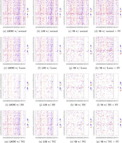
The in-sample estimates highlight three key results. First, there are visible differences across shrinkage priors. For instance, the Horseshoe tend to shrink parameters more aggressively toward zero so that $\widehat{\mathbf{\Theta }}$ is more sparse than, for example, the adaptive Normal-Gamma. Second, consistent with Gefang, Koop, and Poon (2023), the estimates of the LMCMC and LVB tend to be closely related. Yet, these in-sample estimates are substantially different compared to our VB approach. This is due to the parameterization $\widehat{\mathbf{\Theta }}={\widehat{\mathbf{L}}}^{-1}\widehat{\mathbf{A}}$ in (2b). Third, with the exception of the adaptive-Lasso prior, the estimates $\widehat{\mathbf{\Theta }}$ from VB are remarkably stable between constant versus stochastic volatility specifications.

5.2 Out-of-Sample Forecasting Accuracy

Intuitively, different estimates of $\mathbf{\Theta }$ should be reflected in different conditional forecasts. To test this intuition, we now compare the LMCMC, LVB, and the VB estimation approaches with and without stochastic volatility. For completeness, we also consider a series of univariate model specifications (U henceforth), which is akin to assuming conditional independence across industry portfolios. We consider a 360-month rolling window period for each model estimation; for instance, for the 30-industry classification, the out-of-sample period is from July 1957 to May 2020.

Given the recursive nature of the empirical implementation and the extensive out-of-sample period, we do not consider the MCMC approach of Gruber and Kastner (2022). This is because the computational cost would make such implementation prohibitive in practice, as discussed in the simulation study based on Figure 4. For instance, on a 2.5 GHz Intel Xeon W-2175 with 32GB of RAM and 14 cores, it would take $20\min \times 767\text{forecasts}\times 4\text{priors}=61,360$ min, or 42 days, to recursively implement the MCMC approach for the 30 industry portfolios with constant volatility. The computational cost would be even larger when adding stochastic volatility or for the 49 industry portfolios. Appendix E.1 provides a complete discussion of the computational costs of some of the existing MCMC approaches and the key relevance for a higher-frequency forecasting implementation, such as ours.

Point forecasts

We begin by inspecting the accuracy of point forecasts for each industry based on the out-of-sample predictive R² (see, e.g., Goyal and Welch 2008), $$R_{j,\mathit{oos}}^2\left({\mathcal{M}}_s\right)=1-\frac{\sum _{t_0=2}^T{\left(y_{jt}-{\widehat{y}}_{jt}\left({\mathcal{M}}_s\right)\right)}^2}{\sum _{t_0=2}^T{\left(y_{jt}-{\overline{y}}_{jt}\right)}^2},$$where t₀ is the date of the first prediction, ${\overline{y}}_{jt}$ is the naive forecast from the recursive mean–using the same rolling window of observations–and ${\widehat{y}}_{jt}({\mathcal{M}}_s)$ is the conditional mean returns for industry $j=1,\dots ,d$ for a given estimation method ${\mathcal{M}}_s$.

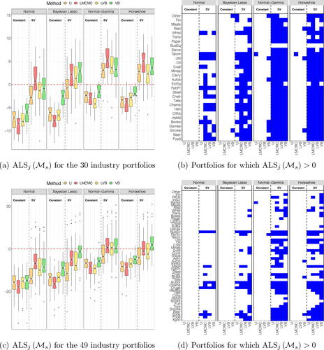
The left panels of Figure 6 show the box charts with the distribution of the $R_{j,\mathit{oos}}^2$ over the $j=1,\dots ,d$ industries. For a given subplot, the results for the Normal, Bayesian Lasso, Normal-Gamma and Horseshoe priors are reported from the left to the right. Within each panel of a subplot, the forecasting results for the U, LMCMC, LVB, and VB estimates are color-coded in orange, red, yellow, and green (from left to right), respectively. The vertical dashed line within each panel separates between constant and stochastic volatility specifications. Based on the same separation across methods and priors, the right panels of Figure 6 report a breakdown of the industries for which $R_{j,\mathit{oos}}^2({\mathcal{M}}_s)>0$.

Fig. 6 Left panels report the $R_{j,\mathit{oos}}^2({\mathcal{M}}_s)$ (in %) across industry portfolios. Right panels report the industries for which a given model can generate $R_{j,\mathit{oos}}^2({\mathcal{M}}_s)>0$. The top (bottom) panels report the results for 30 (49) industry portfolios.

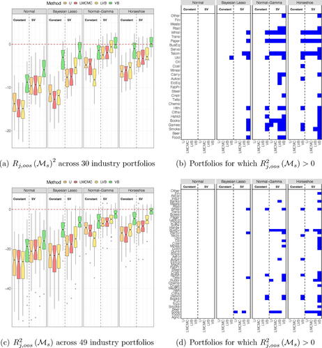
The out-of-sample $R_{j,\mathit{oos}}^2({\mathcal{M}}_s)$ tends to be mostly negative across estimation methods and shrinkage priors. This is consistent with the existing evidence on stock returns predictability: a simple naive forecast based on a rolling sample mean represents a challenging benchmark to beat (see, e.g., Campbell and Thompson 2007). However, our variational inference approach substantially improves upon univariate regressions and the LMCMC, LVB methods, which are both based on a structural VAR representation. For instance, our VB with stochastic volatility generates a positive $R_{j,\mathit{oos}}^2({\mathcal{M}}_s)$ for more than half of the 30 industry portfolios based on the adaptive Normal-Gamma and the Horseshoe. This compares to 4 (adaptive Normal-Gamma) and 3 (Horseshoe) positive $R_{j,\mathit{oos}}^2({\mathcal{M}}_s)$ obtained from LMCMC with stochastic volatility. The gap further increases for the 49-industry classification; our VB method is virtually the only approach that can systematically generate positive $R_{j,\mathit{oos}}^2({\mathcal{M}}_s)$ across industries. Although more concentrated on the Horseshoe prior, the out-performance of our method relative to both LMCMC and VB holds across different priors.

Density forecasts

We follow Fisher et al. (2020) and assess the accuracy of the density forecasts across priors and estimation methods based on the average log-score (ALS) differential with respect to a “no-predictability” benchmark, (15) $${\text{ALS}}_j\left({\mathcal{M}}_s\right)=\frac{1}{T-t_0}\sum _{t_0=2}^T\left(\hspace{0.17em}\ln \hspace{0.17em}{S}_{jt}\left({\mathcal{M}}_s\right)-\hspace{0.17em}\ln \hspace{0.17em}{\overline{S}}_{jt}\right),$$(15) where $\hspace{0.17em}\ln \hspace{0.17em}{S}_{jt}({\mathcal{M}}_s)$ denotes the log-score at time t for industry j obtained by evaluating a Normal density with the conditional mean and variance forecast from the model ${\mathcal{M}}_s$. Consistent with the rationale of the no-predictability benchmark in $R_{j,\mathit{oos}}^2({\mathcal{M}}_s)$, the log-score for $\hspace{0.17em}\ln \hspace{0.17em}{\overline{S}}_{j,t}$ is constructed by evaluating a Normal density based on recursive mean and variance.

Figure 7 reports the results. The labeling is the same as in Figure 6. The results show that by adding stochastic volatility, the accuracy of density forecasts substantially improves across priors and estimation methods. For instance, our VB method with stochastic volatility generates positive log-score differentials for almost all of the portfolios for the 30 industry classification and for more than half of the 49 industry portfolios. Interestingly, when it comes to density forecasts rather than modeling expected returns, the Gefang, Koop, and Poon (2023) variational method built on a structural VAR representation performs on par with our VB method. This is likely due to stochastic volatility alone since our VB still stands out within the constant volatility specifications. Overall, our VB approach outperforms the competing estimation methods under all prior specifications.

Fig. 7 Left panels report the log-score differential across industry portfolios. Right panels report the industries for which a given model can generate a positive log-score differential. The top (bottom) panels report the results for 30 (49) industry portfolios.

Returns predictability over the business cycle

Existing literature suggests that expected returns are counter-cyclical and that returns predictability is more pronounced during periods of economic contractions versus expansions (see, e.g., Rapach, Strauss, and Zhou 2010). Thus, in the following, we investigate if the forecasting performance of our estimation framework changes over the business cycle. More precisely, we split the data into recession and expansionary periods using the NBER dates of peaks and troughs. This information is considered ex-post and is not used at any time in the estimation and/or forecasting process. We compute the corresponding $R_{j,\mathit{oos}}^2({\mathcal{M}}_s)$ for the recession periods only.

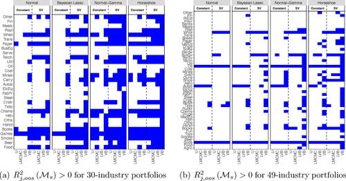
Figure 8 reports the industries for which $R_{j,\mathit{oos}}^2({\mathcal{M}}_s)>0$ for both the 30 (left panel) and the 49 (right panel) industry classification. The corresponding cross-sectional distribution of the $R_{j,\mathit{oos}}^2({\mathcal{M}}_s)$ and the relative log-scores are reported in Appendix E.2. The labeling of Figure 8 is the same as in Figure 6. By comparing Figure 8 with the full sample, the results suggest that the accuracy of the predictions substantially improves across methods and priors. Nevertheless, our VB method outperforms the naive forecast from the rolling mean for a larger fraction of industry portfolios compared to other methods, in particular when stochastic volatility is added to the model. The difference between the recession and the full-sample performance persists when considering the 49 industry classification, especially for the adaptive Normal-Gamma and the Horseshoe prior.

Fig. 8 The figure reports the industries for which $R_{j,\mathit{oos}}^2({\mathcal{M}}_s)>0$. The left (right) panel report the results for 30 (49) industry portfolios.

5.3 Economic Evaluation

A positive predictive performance does not necessarily translate into economic value. However, in practice, an investor is keenly interested in the economic value of returns predictability, perhaps even more than the statistical performance. Hence, it is of paramount importance to evaluate the extent to which apparent gains in predictive accuracy translate into better investment performances.

Following existing literature (see, e.g., Goyal and Welch 2008; Rapach, Strauss, and Zhou 2010), we consider a representative investor with a single-period horizon and mean-variance preferences who allocates her wealth between an industry portfolio and a risk-free asset. Thus, the investor optimal allocation to stocks for period t + 1 based on information at time t is given by $w_{jt}=\frac{1}{\gamma }\frac{{\widehat{y}}_{jt}}{{\widehat{\nu }}_{jt}^{-1}}$, where ${\widehat{y}}_{jt}$ represents the expected return for industry $j=1,\dots ,d$ and ${\widehat{\nu }}_{jt}^{-1}$ the corresponding volatility forecast at time t. We also constrain the weights for each industry to $-0.5\le w_{jt}\le 1.5$ to prevent extreme short sales and leveraged positions. We assume a risk aversion coefficient of γ = 5.

Figure 9 reports the average utility gain—in monthly %—obtained by using a given forecast ${\widehat{y}}_{jt}$ instead of the recursive sample mean ${\overline{y}}_{jt}$. The average utility for a given model is calculated as ${\widehat{u}}_j={\overline{r}}_j-0.5\gamma {\overline{\sigma }}_j^2$ where ${\overline{r}}_j$ and ${\overline{\sigma }}_j^2$ represent the sample mean and variance, respectively, of the portfolio return $r_{jt+1}=w_{jt}{y}_{jt+1}$ realized over the forecasting period for the industry $j=1,\dots ,d$ under a given prior specification and estimation method. The utility gain is calculated by subtracting from the average utility ${\widehat{u}}_j$ the average utility obtained by using the naive forecast from the recursive mean and variance to calculate w_jt. A positive value for the utility gain indicates the fee a risk-averse investor is willing to pay to access the investment strategy implied by ${\mathcal{M}}_s$.

Fig. 9 The left panel reports the cross-sectional distribution of the average utility gain across industry portfolios. The right panel reports the industries for which the utility gain is positive. The top (bottom) panels report the results for the 30-industry (49-industry) classification.

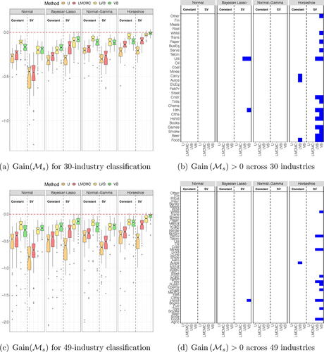
The out-of-sample economic significance largely confirms the statistical performance across methods. From a purely economic standpoint, the forecast from a recursive mean is quite challenging to beat: we observe that the average utility gain is mostly negative, with the only exception of those provided by VB with a Horseshoe prior specification. The results show that a representative investor with mean-variance utility is willing to pay, on average, a monthly fee of almost 15 basis points to access the strategy based on our variational estimation of a large VAR with stochastic volatility. In addition, the right panels of Figure 9 show that the positive economic value obtained from our VB is more broadly spread across industries than alternative methods. This holds especially true for the 30-industry classification but applies to the more granular 49-industry classification.

6 Concluding Remarks

We propose a novel variational Bayes inference method for large-scale VAR with exogenous predictors and stochastic volatility. Different from most existing estimation methods for high-dimensional VAR models, our approach does not rely on a structural form representation. This allows fast and accurate estimation of the model parameters without leveraging on a standard Cholesky-based transformation of the parameter space. We show both in simulation and empirically that our estimation approach outperforms across different prior specifications, both statistically and economically, forecasts from existing benchmark estimation strategies, such as equivalent, nonlinear MCMC algorithms (see, e.g., Gruber and Kastner 2022) linearized MCMC (see, e.g., Cross, Hou, and Poon 2020) and linearized variational inference methods (see, e.g., Gefang, Koop, and Poon 2023).

Supplementary Materials

The supplementary material contains the proof and derivations of all propositions and theoretical results in the paper. The supplementary material contains also additional simulation and empirical results. These additional results have also been briefly discussed in the main text of the paper. The R code pertaining to the variational inference scheme developed in the paper can be found at this link: https://github.com/whitenoise8/Variational-inference-for-large-Bayesian-vector-autoregressions.

Acknowledgments

We are thankful to Andrea Carriero and seminar participants at the 2021 Virtual NBER-NSF SBIES, the 2021 European Summer Meeting of the Econometric Society, the 2nd Workshop on Dimensionality Reduction and Inference in High-Dimensional Time Series at Maastricht University, the 2023 Summer Forum Workshop on Macroeconomics and Policy Evaluation at the Barcelona School of Economics, and the 3rd International Conference on Econometrics and Business Analytics in Tashkent, for their helpful comments and suggestions.

Disclosure Statement

The authors report there are no competing interests to declare.

Additional information

Funding

This research has been partially funded by the BERN_BIRD2222_01 - BIRD 2022 grant from the University of Padua.

References

- Archakov, I., and Hansen, P. R. (2021), “A New Parametrization of Correlation Matrices,” Econometrica, 89, 1699–1715. DOI: 10.3982/ECTA16910.
- Arias, J. E., Rubio-Ramirez, J. F., and Shin, M. (2023), “Macroeconomic Forecasting and Variable Ordering in Multivariate Stochastic Volatility Models,” Journal of Econometrics, 235, 1054–1086. DOI: 10.1016/j.jeconom.2022.04.013.
- Avramov, D. (2004), “Stock Return Predictability and Asset Pricing Models,” Review of Financial Studies, 17, 699–738. DOI: 10.1093/rfs/hhg059.
- Bernardi, M., Bianchi, D., and Bianco, N. (2023), “Dynamic Variable Selection in High-Dimensional Predictive Regressions,” working paper.
- Bognanni, M. (2022), “Comment on “Large Bayesian Vector Autoregressions with Stochastic Volatility and Non-conjugate Priors,” Journal of Econometrics, 227, 498–505. DOI: 10.1016/j.jeconom.2021.10.008.
- Campbell, J. Y., and Thompson, S. B. (2007), “Predicting Excess Stock Returns Out of Sample: Can Anything Beat the Historical Average?” The Review of Financial Studies, 21, 1509–1531. DOI: 10.1093/rfs/hhm055.
- Carriero, A., Clark, T. E., and Marcellino, M. (2019), “Large Bayesian Vector Autoregressions with Stochastic Volatility and Non-conjugate Priors,” Journal of Econometrics, 212, 137–154. DOI: 10.1016/j.jeconom.2019.04.024.
- Carriero, A., Chan, J., Clark, T. E., and Marcellino, M. (2022), “Corrigendum to “Large Bayesian Vector Autoregressions with Stochastic Volatility and Non-conjugate Priors” [j. econometrics 212 (1)(2019) 137–154],” Journal of Econometrics, 227, 506–512. DOI: 10.1016/j.jeconom.2019.04.024.
- Carvalho, C. M., Polson, N. G., and Scott, J. G. (2009), “Handling Sparsity via the Horseshoe,” in Proceedings of the 12th International Conference on Artificial Intelligence and Statistics, April 16–18, 2009 (Vol. 5), pp. 73–80.
- Carvalho, C. M., Polson, N. G., and Scott, J. G. (2010), “The Horseshoe Estimator for Sparse Signals,” Biometrika, 97, 465–480. DOI: 10.1093/biomet/asq017.
- Chan, J. C. (2021), “Minnesota-Type Adaptive Hierarchical Priors for Large Bayesian Vars,” International Journal of Forecasting, 37, 1212–1226. DOI: 10.1016/j.ijforecast.2021.01.002.
- Chan, J. C., and Eisenstat, E. (2018), “Bayesian Model Comparison for Time-Varying Parameter Vars with Stochastic Volatility,” Journal of Applied Econometrics, 33, 509–532. DOI: 10.1002/jae.2617.
- Chan, J. C., and Yu, X. (2022), “Fast and Accurate Variational Inference for Large Bayesian VARs with Stochastic Volatility,” Journal of Economic Dynamics and Control, 143, 104505. DOI: 10.1016/j.jedc.2022.104505.
- Chan, J. C., Koop, G., and Yu, X. (2023), “Large Order-Invariant Bayesian VARs with Stochastic Volatility,” Journal of Business & Economic Statistics, 1–13. DOI: 10.1080/07350015.2023.2252039.
- Cross, J. L., Hou, C., and Poon, A. (2020), “Macroeconomic Forecasting with Large Bayesian VARs: Global-Local Priors and the Illusion of Sparsity,” International Journal of Forecasting, 36, 899–915. DOI: 10.1016/j.ijforecast.2019.10.002.
- Fama, E. F., and French, K. R. (1997), “Industry Costs of Equity,” Journal of Financial Economics, 43, 153–193. DOI: 10.1016/S0304-405X(96)00896-3.
- ———(2015), “A Five-Factor Asset Pricing Model,” Journal of Financial Economics, 116, 1–22.
- Ferson, W. E., and Harvey, C. R. (1991), “The Variation of Economic Risk Premiums,” Journal of Political Economy, 99, 385–415. DOI: 10.1086/261755.
- ———(1999), “Conditioning Variables and the Cross Section of Stock Returns,” The Journal of Finance, 54, 1325–1360.
- Ferson, W. E., and Korajczyk, R. A. (1995), “Do Arbitrage Pricing Models Explain the Predictability of Stock Returns?” Journal of Business, 68, 309–349. DOI: 10.1086/296667.
- Fisher, J. D., Pettenuzzo, D., and Carvalho, C. M. (2020), “Optimal Asset Allocation with Multivariate Bayesian Dynamic Linear Models,” Annals of Applied Statistics, 14, 299–338.
- Gefang, D., Koop, G., and Poon, A. (2023), “Forecasting Using Variational Bayesian Inference in Large Vector Autoregressions with Hierarchical Shrinkage,” International Journal of Forecasting, 39, 346–363. DOI: 10.1016/j.ijforecast.2021.11.012.
- Goyal, A., and Welch, I. (2008), “A Comprehensive Look at the Empirical Performance of Equity Premium Prediction,” The Review of Financial Studies, 21, 1455–1508. DOI: 10.1093/rfs/hhm014.
- Griffin, J. E., and Brown, P. J. (2010), “Inference with Normal-Gamma Prior Distributions in Regression Problems,” Bayesian Analysis, 5, 171–188. DOI: 10.1214/10-BA507.
- Gruber, L., and Kastner, G. (2022), “Forecasting Macroeconomic Data with Bayesian VARs: Sparse or Dense? It depends!,” arXiv preprint arXiv:2206.04902.
- Gunawan, D., Kohn, R., and Nott, D. (2020), “Variational Approximation of Factor Stochastic Volatility Models,” arXiv e-prints, art. arXiv:2010.06738.
- Hahn, P. R., and Carvalho, C. M. (2015), “Decoupling Shrinkage and Selection in Bayesian Linear Models: A Posterior Summary Perspective,” Journal of the American Statistical Association, 110, 435–448. DOI: 10.1080/01621459.2014.993077.
- Hauzenberger, N., Huber, F., and Onorante, L. (2021), “Combining Shrinkage and Sparsity in Conjugate Vector Autoregressive Models,” Journal of Applied Econometrics, 36, 304–327. DOI: 10.1002/jae.2807.
- Hou, K., and Robinson, D. T. (2006), “Industry Concentration and Average Stock Returns,” The Journal of Finance, 61, 1927–1956. DOI: 10.1111/j.1540-6261.2006.00893.x.
- Huber, F., and Feldkircher, M. (2019), “Adaptive Shrinkage in Bayesian Vector Autoregressive Models,” Journal of Business & Economic Statistics, 37, 27–39. DOI: 10.1080/07350015.2016.1256217.
- Huber, F., Koop, G., and Onorante, L. (2021), “Inducing Sparsity and Shrinkage in Time-Varying Parameter Models,” Journal of Business & Economic Statistics, 39, 669–683. DOI: 10.1080/07350015.2020.1713796.
- Kastner, G., and Huber, F. (2020), “Sparse Bayesian Vector Autoregressions in Huge Dimensions,” Journal of Forecasting, 39, 1142–1165. DOI: 10.1002/for.2680.
- Leng, C., Tran, M. N., and Nott, D. (2014), “Bayesian Adaptive Lasso,” Annals of the Institute of Statistical Mathematics, 66, 221–244. DOI: 10.1007/s10463-013-0429-6.
- Lewellen, J., Nagel, S., and Shanken, J. (2010), “A Skeptical Appraisal of Asset Pricing Tests,” Journal of Financial Economics, 96, 175–194. DOI: 10.1016/j.jfineco.2009.09.001.
- Minka, T. P. (2001), “Expectation Propagation for Approximate Bayesian Inference,” in Proceedings of the Seventeenth Conference on Uncertainty in Artificial Intelligence, pp. 362–369.
- Ormerod, J. T., and Wand, M. P. (2010), “Explaining Variational Approximations,” The American Statistician, 64, 140–153. DOI: 10.1198/tast.2010.09058.
- Park, T., and Casella, G. (2008), “The Bayesian Lasso, Journal of the American Statistical Association, 103, 681–686. DOI: 10.1198/016214508000000337.
- Polson, N. G., and Scott, J. G. (2011), “Shrink Globally, Act Locally: Sparse Bayesian Regularization and Prediction,” in Bayesian Statistics, 9, 501–538.
- Rapach, D., and Zhou, G. (2013), “Forecasting Stock Returns,” in Handbook of Economic Forecasting (Vol. 2), eds. G. Elliott and A. Timmermann, pp. 328–383, Amsterdam: Elsevier.
- Rapach, D. E., Strauss, J. K., and Zhou, G. (2010), “Out-of-Sample Equity Premium Prediction: Combination Forecasts and Links to the Real Economy,” The Review of Financial Studies, 23, 821–862. DOI: 10.1093/rfs/hhp063.
- Ray, P., and Bhattacharya, A. (2018), “Signal Adaptive Variable Selector for the Horseshoe Prior,” arXiv: Methodology.
- Rohde, D., and Wand, M. P. (2016), “Semiparametric Mean Field Variational Bayes: General Principles and Nmerical Issues,” The Journal of Machine Learning Research, 17, 5975–6021.
- Rothman, A. J., Levina, E., and Zhu, J. (2010), “A New Approach to Cholesky-based Covariance Regularization in High Dimensions,” Biometrika, 97, 539–550. DOI: 10.1093/biomet/asq022.
- Wand, M. P., Ormerod, J. T., Padoan, S. A., and Frührwirth, R. (2011), “Mean Field Variational Bayes for Elaborate Distributions,” Bayesian Analysis, 6, 847–900. DOI: 10.1214/11-BA631.