Unconditional Quantile Regression for Streaming Datasets

Abstract

The Unconditional Quantile Regression (UQR) method, initially introduced by Firpo et al. has gained significant traction as a popular approach for modeling and analyzing data. However, much like Conditional Quantile Regression (CQR), UQR encounters computational challenges when it comes to obtaining parameter estimates for streaming datasets. This is attributed to the involvement of unknown parameters in the logistic regression loss function used in UQR, which presents obstacles in both computational execution and theoretical development. To address this, we present a novel approach involving smoothing logistic regression estimation. Subsequently, we propose a renewable estimator tailored for UQR with streaming data, relying exclusively on current data and summary statistics derived from historical data. Theoretically, our proposed estimators exhibit equivalent asymptotic properties to the standard version computed directly on the entire dataset, without any additional constraints. Both simulations and real data analysis are conducted to illustrate the finite sample performance of the proposed methods.

Keywords:

• Renewable estimation
• Smoothing method
• Streaming datasets
• Unconditional quantile regression

1 Introduction

Quantile regression (QR) models proposed by Koenker and Bassett (1978) are more robust to outliers than the classical mean regression models, and any quantile can be used in any part of the outcome distribution. The most commonly used QR framework is the conditional quantile regression (CQR). It is used to assess the impact of a covariate on a quantile of the outcome conditional on specific values of other covariates (Jiang and Yu 2023). CQR is widely seen as an ideal tool to understand complex predictor-response relations, however, CQR models do not average up to their unconditional population counterparts. As a result, the estimates obtained cannot be used to estimate the impacts of an explanatory variable X on the corresponding unconditional quantile of the outcome variable Y. To overcome this restriction, Firpo et al. (2009) proposed a regression of the (recentered) influence function of the unconditional quantile of the Y on the X, or UQR estimates the impact of changing the distribution of Y on marginal distribution of X. The advantage of the UQR model is that the quantiles are defined preregression; therefore, the model is not influenced by any right-hand-side variables. In UQR, one can, for instance, include fixed effects to adjust for selection bias without redefining the quantiles (Borgen 2016). The UQR method has attracted substantial attention in statistics and econometrics with many applications in different fields. By January 2023, Firpo et al. (2009) has attracted 2500+ Google Scholar citations, such as Ghosh (2021), Inoue, Li, and Xu (2021), Sasaki, Ura, and Zhang (2022), and Martinez-Iriarte, Montes-Rojas, and Sun (2022) and so on.

In spite of its rapidly growing popular method for modeling and analyzing data, however, UQR faces challenges to obtaining parameter estimates from “big data.” The concept of “big data” may have different meanings to people from different fields and has since become a dominant topic in nearly all academic disciplines and in applied fields. In a broad sense, big data is data on a larger scale in terms of volume, variety, velocity, variability, and veracity. In this article, we consider one type of big data: streaming data, which grows rapidly in volume and velocity. Due to the explosive growth of data onto nontraditional sources such as mobile phones, social networks and e-commerce, streaming data is becoming a core component of big data analysis.

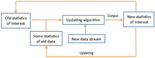
Streaming data grows rapidly in volume and velocity. Then storing and combing data becomes increasingly challenging. To reduce the demand on computing memory and achieve real-time processing, the nature of streaming data calls for the development of algorithms which require only “one pass” over the data. This means that in order to reduce storage requirements and computation time, data is only used once. Therefore, the primary goal of processing such streaming data is to sequentially update some statistics of interest upon the arrival of a new data batch, in the hope to not only free up space for the storage of massive historical individual-level data, but also provide real-time inference and decision-making. Online updating approaches are distinct from the massive data analysis because they target problem where data arrive in streams or large chunks and address statistical problems in an updating framework without storage requirements for previous data, as shown in Figure 1. There are three online updating methods for analyzing streaming data in the literature as follows: average updating methods (Schifano et al. 2016), subsampling methods (Xie, Bai, and Ma 2023) and renewable methods based on estimation equations (Luo and Song 2020). The average updating methods developed in Schifano et al. (2016) require the total number of batches smaller than the sample size of each batch to establish the same statistical properties as that of the oracle estimators with the full datasets, see Theorem B.1 in the Appendix, supplementary materials. This means that streaming data cannot be unlimited, which is not very suitable for the practical application of streaming data. The estimators obtained by subsampling-based approaches are $\sqrt{\tilde{n}}$-consistent instead of $\sqrt{n}$-consistent, where $\tilde{n}$ is the sample size of subsample and n is the sample size of all data, see Wang, Min, and Stufken (2019) and Xie, Bai, and Ma (2023). This means that there is information loss in this method. The estimators obtained by the renewable methods based on estimation equations in Luo and Song (2020) can achieve $\sqrt{n}$-consistent and overcome the above unnatural restriction for average updating methods. Other references on the online updating methods can see Deshpande, Javanmard, and Mehrabi (2023), Luo, Zhou, and Song (2023), Yang and Yao (2023) and so on.

Fig. 1 Online-updating algorithm for streaming datasets.

Specifically, the difficulties faced in analyzing UQR under streaming data are as follows.

First, it is difficult to perform standard logistic regression based on the loss function (3.4) in Section 3 under streaming data according to the term $\mathrm{I}(Y_i>{\tilde{q}}_{\tau })$. Although the method in Luo and Song (2020) can be used to construct a renewable estimator, due to the term $\mathrm{I}(Y_i>{\tilde{q}}_{\tau })$, the error of the estimator of ${\mathit{\beta }}_{q_{\tau }}$ increases as the number of streams increases. To solve the above problem, we adopt a smoothing technique to smooth the above indicative function, which helps to reduce the error from $O_p(|{\tilde{q}}_{\tau }-q_{\tau }|)$ to $O_p(|{\tilde{q}}_{\tau }-q_{\tau }{|}^2)$, so that the error can be ignored. The smoothing technique are often used in QR, see Horowitz (1998), Chen, Liu, and Zhang (2019), Fernandes, Guerre, and Horta (2021), He et al. (2023) and so on. But, to the best of our limited knowledge, there is no literature on the application of smoothing technique to UQR.

Second, as we all known that the bandwidth h is important for the kernel density estimator (3.6) in Section 3, and it depends on the sample size. For streaming data, we cannot know the total sample size at the beginning, so h needs to change with the arrival of new data. Kong and Xia (2019) developed an online density estimate with a single point of update. In this article, we extend the single point update estimation method to batch update estimation. Moreover, the kernel density estimator (3.6) contains ${\tilde{q}}_{\tau }$, thus, we take Taylor expansion to construct a renewable estimator.

Finally, the unconditional quantile partial effect defined in (3.3) involves the quantile of Y. The above methods for streaming data based on the least squares or estimating equations are not suitable for the QR because the quantile regression estimator has no display expression like the least squares estimator and the loss function of the quantile regression is not differentiable, even though loss function needs to be second-order differentiable in the estimation equation (Luo and Song 2020). In order to overcome the non-differentiable of the QR loss function, Jiang and Yu (2022) used a convolution-type smoothing method to develop a renewable estimation. Chen, Liu, and Zhang (2019) and Wang, Wang, and Li (2022) also studied QR estimation for streaming data. However, their methods are all required additional strict conditions on the sample size of each bath. In this article, we adjust method of Jiang and Yu (2022) to estimate $q_{\tau }$ in the (3.3).

To summarize, we develop a renewable estimation for UQR. Our statistical contributions include: (i) Note that the loss function (3.4) in Section 3 is different to the standard logistic regression according to the term $\mathrm{I}(Y_i>{\tilde{q}}_{\tau })$. Therefore, the method of Luo and Song (2020) does not work. To solve the above problem, we adopt a smoothing technique to smooth the above indicative function, which helps to produce a renewable estimator. (ii) We develop a renewable kernel density estimator and a renewable QR estimator. (iii) We propose a renewable UQR estimation that only requires the availability of the current data batch in the data stream and sufficient statistics on the historical data at each stage of the analysis. The asymptotic properties of the proposed renewable estimator under the conditions are similar to those in an offline setting and no restrictions on number of batches, which means that the new methods are adaptive to the situation where streaming datasets arrive fast and perpetually.

The remainder of this article is organized as follows. Section 2 presents a motivational example. The review of the standard UQR is given in Section 3. In Section 4, the streaming datasets analysis method is proposed. Both simulation studies and empirical applications are given in Sections 5 and 6 to illustrate the proposed procedures. We conclude the article with a brief discussion in Section 7. All technical proofs are deferred to the Appendix, supplementary materials.

2 Motivating Example

We exemplify the application of streaming data in economics using the following stock price and exchange rate data.

As the process of financial globalization continues to deepen, the financial markets of various countries become increasingly interconnected, underscoring the pivotal role of the exchange rate system in the capital market. The exchange rate represents the international price of a country’s currency. Changes in the exchange rate signify alterations in the international purchasing power of the currency, making it a crucial policy tool for maintaining national economic security and ensuring financial stability. Stock prices act as a “barometer” of macroeconomics, offering timely reflections of microeconomic changes. The fluctuation in exchange rates not only impacts the macroeconomic operations of a country but also influences the behavior of microeconomic entities, subsequently affecting the stock prices of companies. A comprehensive understanding of the relationship between exchange rates and stock indexes is instrumental for countries and international organizations to manage their exposure to foreign exchange risks. Moreover, it proves invaluable for investors seeking to hedge or predict returns on their foreign investments.

The relationship between the foreign exchange market and the stock market has garnered significant attention from scholars. Bahmani-Oskooee and Sohrabian (1992) used Granger causality tests and co-integration methods to investigate the connection between the foreign exchange market and the stock market in the United States. The research indicates the presence of a short-term two-way causal relationship. Pan, Fok, and Liu (2007) delved into East Asia using data from January 1988 to October 1998, discovering that, before the Asian financial crisis in 1997, there was a causal relationship from the exchange rate to the stock market in Hong Kong, Japan, Malaysia, and Thailand. Additionally, there was a causal relationship from the stock market to the exchange rate in Hong Kong, South Korea, and Singapore. Amba and Nguyen (2019) examined the relationship between stock prices and exchange rates in the Mexican and Canadian markets, employing weekly data from January 2013 to December 2018. The Granger causality test affirmed the existence of a short-term one-way causal relationship between exchange rates and stock prices in the Mexican market.

In this section, we will provide a detailed introduction to the Chinese A-share stock market and explore the relationship between daily stock returns and exchange rates. China’s A-share stock market, encompassing the Shenzhen Stock Exchange and Shanghai Stock Exchange, was officially established in 1990. The trading data within the stock industry is substantial, reaching the gigabyte level. As of March 31, 2023, the A-share market in China comprises 4495 stocks, with 1824 listed on the Shanghai Stock Exchange and 2671 on the Shenzhen Stock Exchange. A study by Zhang and Li (2010) investigated the correlation between exchange rate changes and the stock market in China post the reform of the exchange rate system and the split structure of the stock market in 2005. The study revealed a long-term co-integration relationship between the exchange rate and the stock market. The results indicate that, in the long run, the relationship between exchange rate changes and the stock market primarily follows the flow-oriented model, with the Shanghai A-share index being more noticeably affected by exchange rates. Both stock transaction and exchange rate datasets undergo real-time changes with each transaction, adhering to the typical characteristics of streaming data: (a) the data object is real-time and online; (b) the scale of the data is extensive and theoretically limitless, making it optimal to read each data object only once, thereby reducing data storage requirements. Simultaneously, both institutional and individual investors seek real-time insights into the stock market. Consequently, the analysis of stock trading data should offer real-time analysis functions. Fulfilling these requirements is unattainable with traditional data analysis techniques.

For instance, when examining the relationship between the daily returns in the Shanghai Stock Exchange in China and the exchange rate between the Chinese currency and the US dollar, we can collect approximately 1600 data points per day (excluding suspended trading and stocks under special treatment). Considering the 871 trading days between January 1, 2020, and August 25, 2023, the total data volume amounts to 1,339,591. If we break down the data per minute, the volume becomes $1339591\times 4\times 60=321,501,840$ (accounting for the 4 hr of daily trading). As established in Section 6.2, analyzing 1,339,591 data points takes 65.37 sec, indicating that processing minute-level data, totaling 321,501,840, would certainly exceed a minute, which is deemed unacceptable. However, employing stream data analysis techniques, specifically update estimation methods, allows for the processing of the last batch of incoming data and some statistics from past data, resulting in an analysis time of just 0.02 sec. Whether considering daily or minute data, the volume of the last batch typically hovers around 1600, making this approach highly efficient.

3 Standard Unconditional Quantile Regression

In this section, we first review the standard unconditional quantile regression with full data (assuming that streaming data can be pooled into a dataset and can be analyzed and stored by a computer). Consider a general structural model: (3.1) $$\begin{array}{c}\mathit{Y}=g(\mathit{X},\mathit{\epsilon }),\hfill \end{array}$$(3.1) where the unknown mapping $g(·,·)$ is invertible on the second argument, $\mathit{\epsilon }$ is an unobservable determinant of the outcome variable Y and X is a p-dimensional covariates.

According to the definition in Firpo et al. (2009), we use another name unconditional quantile partial effect ($\mathbf{UQPE}$) for UQR. The $\mathbf{UQPE}$ at quantile level τ proposed by Firpo et al. (2009) is defined as $$\begin{array}{cc}\mathbf{UQP}{\mathbf{E}}_{\tau }=\hfill & \int \frac{d\mathrm{E}\{\mathbf{RIF}(\mathit{Y},q_{\tau })|\mathit{X}=\mathit{x}\}}{d\mathit{x}}d{F}_{\mathit{X}}(\mathit{x})\hfill \\ =\hfill & \frac{1}{f_{\mathit{Y}}(q_{\tau })}\int \frac{d\mathrm{E}\{\mathrm{I}(\mathit{Y}>q_{\tau })|\mathit{X}=\mathit{x}\}}{d\mathit{x}}d{F}_{\mathit{X}}(\mathit{x}),\hfill \end{array}$$where $F_{\mathit{X}}(·)$ is the distribution function of X, $\mathbf{RIF}(y,q_{\tau })=\mathrm{I}(y>q_{\tau })/f_{\mathit{Y}}(q_{\tau })+q_{\tau }-(1-\tau )/f_{\mathit{Y}}(q_{\tau })$ is the recentered influence function, $\mathrm{I}(·)$ is the indicator function, $q_{\tau }$ and $f_{\mathit{Y}}(·)$ are the τth quantile and the density function of Y, respectively. Assume that (3.2) $$\begin{array}{c}\mathrm{P}\left(\mathit{Y}>q_{\tau }|\mathit{X}=\mathit{x}\right)=\Lambda ({\mathit{x}}^{\top }{\mathit{\beta }}_{q_{\tau }}),\hfill \end{array}$$(3.2) where ${\mathit{\beta }}_{q_{\tau }}\mathrm{}=\mathrm{}\arg {\max }_{\mathit{\beta }}\mathrm{E}\left[\mathrm{I}(\mathit{Y}\mathrm{}>\mathrm{}{q}_{\tau })·{\mathit{X}}^{\top }\mathit{\beta }+\hspace{0.17em}\log \hspace{0.17em}\{1-\Lambda ({\mathit{X}}^{\top }\mathit{\beta })\}\right]$ and $\Lambda (r)=1/(1+e^{-r})$ is the logistic distribution function. Then, by the assumption (3.2), $\mathbf{UQP}{\mathbf{E}}_{\tau }$ is equal to (3.3) $$\begin{array}{c}\mathbf{UQP}{\mathbf{E}}_{\tau }=\frac{{\mathit{\beta }}_{q_{\tau }}}{f_{\mathit{Y}}(q_{\tau })}\int \Lambda \prime ({\mathit{x}}^{\top }{\mathit{\beta }}_{q_{\tau }})d{F}_{\mathit{X}}(\mathit{x}),\hfill \end{array}$$(3.3) where $\Lambda \prime (r)=\Lambda (r)\{1-\Lambda (r)\}$ is the derivative of $\Lambda (r)$. Note that the assumption (3.2) is the assumption 11 in Firpo et al. (2009) and (3.3) is the RIF-Logit in Firpo et al. (2009).

We first review the standard estimation method of $\mathbf{UQP}{\mathbf{E}}_{\tau }$ in Firpo et al. (2009). Let ${\{{\mathit{X}}_i,Y_i\}}_{i=1}^n$ be an iid sample from $(\mathit{X},\mathit{Y})$ in model (3.1). Based on the assumption (3.2), the estimator of ${\mathit{\beta }}_{q_{\tau }}$ based on ${\tilde{q}}_{\tau }$ is (3.4) $$\begin{array}{c}{\tilde{\mathit{\beta }}}_{{\tilde{q}}_{\tau }}=\arg {\max }_{\mathit{\beta }}\sum _{i=1}^n\left[\mathrm{I}(Y_i>{\tilde{q}}_{\tau })·{\mathit{X}}_i^{\top }\mathit{\beta }+\hspace{0.17em}\log \hspace{0.17em}\{1-\Lambda ({\mathit{X}}_i^{\top }\mathit{\beta })\}\right],\hfill \end{array}$$(3.4) where ${\tilde{q}}_{\tau }$ is the estimator of $q_{\tau }$ as (3.5) $$\begin{array}{c}{\tilde{q}}_{\tau }=\arg {\min }_q\sum _{i=1}^n{\rho }_{\tau }\left(Y_i-q\right),\hfill \end{array}$$(3.5) where ${\rho }_{\tau }(r)=\tau r-r\mathrm{I}(r<0)$ is the check loss function. Moreover, the kernel density estimator for the density of Y at ${\tilde{q}}_{\tau }$ is (3.6) $$\begin{array}{c}{\tilde{f}}_{\mathit{Y}}({\tilde{q}}_{\tau })=\frac{1}{n}\sum _{i=1}^n{K}_h\left(Y_i-{\tilde{q}}_{\tau }\right),\hfill \end{array}$$(3.6) where $K_h(·)=K(·/h)/h,K(·)$ is a smooth kernel function and h is a bandwidth.

Then, the estimator of $\mathbf{UQP}{\mathbf{E}}_{\tau }$ based on (3.3)–(3.6) is (3.7) $$\begin{array}{c}{\widetilde{\mathbf{UQPE}}}_{\tau }=\frac{{\tilde{\mathit{\beta }}}_{{\tilde{q}}_{\tau }}}{{\tilde{f}}_{\mathit{Y}}({\tilde{q}}_{\tau })}\frac{1}{n}\sum _{i=1}^n\Lambda \prime ({\mathit{X}}_i^{\top }{\tilde{\mathit{\beta }}}_{{\tilde{q}}_{\tau }}).\hfill \end{array}$$(3.7)

4 Streaming Datasets Analysis

Now let us discuss how to develop a renewable estimator for $\mathbf{UQPE}$ based on streaming datasets. Assume we have the streaming datasets $\{{\mathit{D}}_1,\dots ,{\mathit{D}}_b\}$ up to the bth batch, where ${\mathit{D}}_j=\{({\mathit{X}}_{i,j},Y_{i,j}),i=1,\dots ,N_j\}$ is the jth batch dataset with a sample size of N_j. We suppose that the $({\mathit{X}}_{i,j},Y_{i,j})$ for all is and js are iid samples from $(\mathit{X},\mathit{Y})$ in model (3.1). The sample size up to the bth batch is ${\overline{N}}_b={\sum }_{j=1}^b{N}_j$.

The key idea of the following renewable estimation is to use the Taylor expansion of the score function so that the new estimation equation uses only the combined information of the previous data and the data of the current batch. In the non-differentiable case, smoothing techniques will be used to enable Taylor expansion of the scoring function.

4.1 Estimate $q_{\tau }$ for Streaming Datasets

Note that for a quantile regression, the loss function ${\rho }_{\tau }(r)=\tau r-r\mathrm{I}(r<0)$ is non-differentiable. Therefore, the QR estimator has no display expression, so it is impossible to construct a renewable estimator for streaming data. To circumvent the non-differentiable of the QR loss function, we smooth quantile regression loss function ${\rho }_{\tau }(r)$ to a twice continuously differentiable function (Nadaraya 1964; Fernandes, Guerre, and Horta 2021): (4.1) $$\begin{array}{c}{\mathbf{Q}}_h(r)=\int {\rho }_{\tau }(t)K_h(t-r)dt.\hfill \end{array}$$(4.1)

For example, we take Logistic kernel $K(u)=e^{-u}/{(1+e^{-u})}^2$ in (4.1), the explicit expression of ${\mathbf{Q}}_h(r)$ is $\tau r+h\hspace{0.17em}\log \hspace{0.17em}(1+e^{-r/h})$. By (4.1), the ${\widehat{q}}_{\tau }^1$ based on ${\mathit{D}}_1$ satisfies, (4.2) $$\begin{array}{c}\sum _{i\in {\mathit{D}}_1}\left\{\tilde{K}(({\widehat{q}}_{\tau }^1-Y_i)/h_{q,1})-\tau \right\}=0,\hfill \end{array}$$(4.2) which is the derivative of ${\mathbf{Q}}_h(·)$ on dataset ${\mathit{D}}_1$, and where $\tilde{K}(r)={\int }_{-\infty }^{r}K(u)du$ and $h_{q,j}$ is a bandwidth for jth batch. We propose a new estimator ${\widehat{q}}_{\tau }^2$ for streaming data $\{{\mathit{D}}_1,{\mathit{D}}_2\}$ as a solution to the equation of the form (4.3) $$\begin{array}{c}\sum _{i\in {\mathit{D}}_1}{K}_{h_{q,1}}({\widehat{q}}_{\tau }^1-Y_i)({\widehat{q}}_{\tau }^2-{\widehat{q}}_{\tau }^1)\\ +\sum _{i\in {\mathit{D}}_2}\left\{\tilde{K}(({\widehat{q}}_{\tau }^2-Y_i)/h_{q,2})-\tau \right\}=\mathbf{0},\end{array}$$(4.3) which is according to $$\begin{array}{c}\sum _{i\in {\mathit{D}}_1}\left\{\tilde{K}(({\widehat{q}}_{\tau }^2-Y_i)/h_{q,1})-\tau \right\}\\ =\sum _{i\in {\mathit{D}}_1}\left\{\tilde{K}(({\widehat{q}}_{\tau }^1-Y_i)/h_{q,1})-\tau \right\}\\ +\sum _{i\in {\mathit{D}}_1}{K}_{h_{q,1}}({\widehat{q}}_{\tau }^1-Y_i)({\widehat{q}}_{\tau }^2-{\widehat{q}}_{\tau }^1)+O_p(N_1|{\widehat{q}}_{\tau }^2-{\widehat{q}}_{\tau }^1{|}^2)\\ =\sum _{i\in {\mathit{D}}_1}{K}_{h_{q,1}}({\widehat{q}}_{\tau }^1-Y_i)({\widehat{q}}_{\tau }^2-{\widehat{q}}_{\tau }^1)+O_p(N_1|{\widehat{q}}_{\tau }^2-{\widehat{q}}_{\tau }^1{|}^2),\end{array}$$ where the last equation is according to (4.2), $O_p(·)$ means bounded with probability and the error term $O_p(N_1|{\widehat{q}}_{\tau }^2-{\widehat{q}}_{\tau }^1{|}^2)$ is asymptotically ignored.

Generalizing (4.3) to streaming datasets $\{{\mathit{D}}_1,\dots ,{\mathit{D}}_b\}$, a renewable estimator ${\widehat{q}}_{\tau }^b$ of $q_{\tau }$ is defined as a solution to the following incremental estimation equation: (4.4) $$\begin{array}{c}{\widehat{\mathit{K}}}^{b-1}({\widehat{q}}_{\tau }^b-{\widehat{q}}_{\tau }^{b-1})+\sum _{i\in {\mathit{D}}_b}\left\{\tilde{K}\left(\frac{{\widehat{q}}_{\tau }^b-Y_i}{h_{q,b}}\right)-\tau \right\}=\mathbf{0},\hfill \end{array}$$(4.4) where ${\widehat{\mathit{K}}}^{b-1}={\sum }_{j=1}^{b-1}\sum _{i\in {\mathit{D}}_j}{K}_{h_{q,j}}({\widehat{q}}_{\tau }^j-Y_i)$. The asymptotic property of ${\widehat{q}}_{\tau }^b$ can see Lemma 2 in the Appendix, supplementary materials. Numerically, it is quite straightforward to find ${\widehat{q}}_{\tau }^b$ from (4.4) using the Newton-Raphson method as (4.5) $$\begin{array}{c}{\widehat{q}}_{\tau }^b={\widehat{q}}_{\tau }^{b-1}-{\left\{{\widehat{\mathit{K}}}^{b-1}+\sum _{i\in {\mathit{D}}_b}{K}_{h_{q,j}}({\widehat{q}}_{\tau }^{b-1}-Y_i)\right\}}^{-1}\\ \hspace{1em}\sum _{i\in {\mathit{D}}_b}\left\{\tilde{K}\left(\frac{{\widehat{q}}_{\tau }^{b-1}-Y_i}{h_{q,b}}\right)-\tau \right\}.\end{array}$$(4.5)

Only one iteration in (4.5) is due to that ${\widehat{q}}_{\tau }^b$ is $\sqrt{{\overline{N}}_b}$-consistent by Lemma 2 in the Appendix, supplementary materials and condition $N_j=O(N_1)$ for $j=1,\dots ,b$. Therefore, the estimators ${\widehat{q}}_{\tau }^b$ can converge in one iteration.

4.2 Estimate $f_{\mathbf{Y}}(q_{\tau })$ for Streaming Datasets

It is easy to estimate $f_{\mathit{Y}}(q_{\tau })$ based on the first batch as ${\widehat{f}}_{\mathit{Y}}^1=N_1{}^{-1}\sum _{i\in {\mathit{D}}_1}{K}_{h_{f,1}}(Y_i-{\widehat{q}}_{\tau }^1),$ where $h_{f,j}$ is a bandwidth for the jth batch. When the next data ${\mathit{D}}_2$ arrive, the estimator of $f_{\mathit{Y}}(q_{\tau })$ should be $$\begin{array}{c}\frac{1}{{\overline{N}}_2}\left\{\sum _{i\in {\mathit{D}}_1}{K}_{h_{f,2}}(Y_i-{\widehat{q}}_{\tau }^2)+\sum _{i\in {\mathit{D}}_2}{K}_{h_{f,2}}(Y_i-{\widehat{q}}_{\tau }^2)\right\}.\hfill \end{array}$$

As we all known that we can not know the sample size of next batch, thus, it is difficult to use $h_{f,2}$ in ${\mathit{D}}_1$ because of $h_{f,2}$ always depending on ${\overline{N}}_2$. We will prove in Theorem 4.1 that the following estimator is also effective $$\begin{array}{c}\frac{1}{{\overline{N}}_2}\left\{\sum _{i\in {\mathit{D}}_1}{K}_{h_{f,1}}(Y_i-{\widehat{q}}_{\tau }^2)+\sum _{i\in {\mathit{D}}_2}{K}_{h_{f,2}}(Y_i-{\widehat{q}}_{\tau }^2)\right\}.\hfill \end{array}$$

Moreover, we use Taylor expansion to ${\widehat{q}}_{\tau }^2$ in ${\mathit{D}}_1$ as $$\begin{array}{c}\sum _{i\in {\mathit{D}}_1}{K}_{h_{f,1}}(Y_i-{\widehat{q}}_{\tau }^2)=\sum _{i\in {\mathit{D}}_1}{K}_{h_{f,1}}(Y_i-{\widehat{q}}_{\tau }^1)\\ +\sum _{i\in {\mathit{D}}_1}{h}_{f,1}^{-1}K{\prime }_{h_{f,1}}(Y_i-{\widehat{q}}_{\tau }^1)({\widehat{q}}_{\tau }^1-{\widehat{q}}_{\tau }^2)+O_p(N_1{h}_{f,1}^{-2}|{\widehat{q}}_{\tau }^1-{\widehat{q}}_{\tau }^2{|}^2),\end{array}$$where $K\prime (·)$ is the derivative of $K(·)$ and $K{\prime }_h(·)=K\prime (·/h)/h$. Then, we can obtain the estimator of $f_{\mathit{Y}}(q_{\tau })$ based on ${\mathit{D}}_1$ and ${\mathit{D}}_2$ as $$\begin{array}{c}{\widehat{f}}_{\mathit{Y}}^2=\frac{1}{{\overline{N}}_2}\sum _{j=1}^2\sum _{i\in {\mathit{D}}_j}{K}_{h_{f,j}}(Y_i-{\widehat{q}}_{\tau }^j)+\frac{1}{{\overline{N}}_2}\\ \hspace{1em}\sum _{i\in {\mathit{D}}_1}{h}_{f,1}^{-1}K{\prime }_{h_{f,1}}(Y_i-{\widehat{q}}_{\tau }^1)({\widehat{q}}_{\tau }^1-{\widehat{q}}_{\tau }^2).\end{array}$$

Generalizing the above method to streaming datasets $\{{\mathit{D}}_1,\dots ,{\mathit{D}}_b\}$, a renewable estimator ${\widehat{f}}_{\mathit{Y}}^b$ of $f_{\mathit{Y}}(q_{\tau })$ is defined as (4.6) $$\begin{array}{c}{\widehat{f}}_{\mathit{Y}}^b=\frac{1}{{\overline{N}}_b}\sum _{j=1}^b\sum _{i\in {\mathit{D}}_j}{K}_{h_{f,j}}(Y_i-{\widehat{q}}_{\tau }^j)\\ +\frac{1}{{\overline{N}}_b}\sum _{j=1}^{b-1}\sum _{i\in {\mathit{D}}_j}{h}_{f,j}^{-1}K{\prime }_{h_{f,j}}(Y_i-{\widehat{q}}_{\tau }^j)({\widehat{q}}_{\tau }^j-{\widehat{q}}_{\tau }^b)\\ =\frac{1}{{\overline{N}}_b}\left\{{\mathit{K}}_1^{b-1}+{\mathit{K}}_2^{b-1}-{\widehat{q}}_{\tau }^b{\mathit{K}}_3^{b-1}+\sum _{i\in {\mathit{D}}_b}{K}_{h_{f,b}}(Y_i-{\widehat{q}}_{\tau }^b)\right\},\end{array}$$(4.6) where ${\mathit{K}}_1^{b-1}={\sum }_{j=1}^{b-1}\sum _{i\in {\mathit{D}}_j}{K}_{h_{f,j}}(Y_i-{\widehat{q}}_{\tau }^j),{\mathit{K}}_2^{b-1}={\sum }_{j=1}^{b-1}\sum _{i\in {\mathit{D}}_j}{h}_{f,j}^{-1}K{\prime }_{h_{f,j}}(Y_i-{\widehat{q}}_{\tau }^j){\widehat{q}}_{\tau }^j$ and ${\mathit{K}}_3^{b-1}={\sum }_{j=1}^{b-1}\sum _{i\in {\mathit{D}}_j}{h}_{f,j}^{-1}K{\prime }_{h_{f,j}}(Y_i-{\widehat{q}}_{\tau }^j)$.

The item ${\overline{N}}_b{}^{-1}{\sum }_{j=1}^b\sum _{i\in {\mathit{D}}_j}{K}_{h_{f,j}}(Y_i-{\widehat{q}}_{\tau }^j)$ in (4.6) is to extend the single point update estimation method in Kong and Xia (2019) to batch update estimation, and the term ${\overline{N}}_b{}^{-1}{\sum }_{j=1}^{b-1}\sum _{i\in {\mathit{D}}_j}{h}_{f,j}^{-1}K{\prime }_{h_{f,j}}(Y_i-{\widehat{q}}_{\tau }^j)({\widehat{q}}_{\tau }^j-{\widehat{q}}_{\tau }^b)$ makes approximate to the density estimation of point ${\widehat{q}}_{\tau }^b$. To reveal the merits of the proposed method, we now establish the asymptotic normality of ${\widehat{f}}_{\mathit{Y}}^b$.

To establish the asymptotic properties of the proposed estimator, the following technical conditions are imposed.

C1. Density function $f_{\mathit{Y}}(·)$ is positive and has second-order derivative, whose second-order derivative is bounded and continuous in a neighborhood of a grid of selected points $q_{\tau }\in \mathfrak{R}$. Moreover, $\int |f_{\mathit{Y}}(y)|dy<\infty$.

C2. The kernel function $K(·)$ is even, integrable, and twice differentiable with bounded first and second derivatives such that $\int K(u)du=1,\int |u^{2}K(u)|du<\infty ,\int uK(u)du=0$ and $\int u^{2}K(u)du\ne 0$.

Remark 4.1.

Conditions C1 and C2 are Assumptions 2, 3, 6, and 7 in Firpo et al. (2009). The Logistic kernel $K(u)=e^{-u}/{(1+e^{-u})}^2$ satisfies condition C2.

Theorem 4.1.

Assume that conditions C1 and C2 hold. If $N_j=O(N_1)$ and $N_1\to \infty ,h_{f,j}=O({\overline{N}}_j^{-c_1})$ with $0<c_1<1/4$ and ${\overline{N}}_j={\sum }_{i=1}^j{N}_i$ for $j=1,\dots ,b$, where b can be a fixed number or a divergent number, we have $$\begin{array}{c}\sqrt{{\overline{N}}_b{h}_{{\overline{N}}_b}}\left({\widehat{f}}_{\mathit{Y}}^b-f_{\mathit{Y}}(q_{\tau })-\frac{1}{2}f\prime {\prime }_{\mathit{Y}}(q_{\tau }){\mu }_K\sum _{j=1}^b\frac{N_j}{{\overline{N}}_b}{h}_{f,j}^2\right)\stackrel{L}{\to }\\ \text{\hspace{1em}\hspace{1em}N}\left(\mathit{0},f_{\mathit{Y}}(q_{\tau }){\nu }_K\right),\end{array}$$where $h_{{\overline{N}}_b}={\overline{N}}_b/{\sum }_{j=1}^b{N}_j{h}_{f,j}^{-1},{\mu }_K=\int u^{2}K(u)du,{\nu }_K=\int K^2(u)du$ and $a_n=O(b_n)$ means $\underset{n}{\sup }|a_n/b_n|<c<\infty$ with a positive and bounded constant c.

If $1/5<c_1<1/4$, we have $$\begin{array}{c}\sqrt{{\overline{N}}_b{h}_{{\overline{N}}_b}}\left({\widehat{f}}_{\mathit{Y}}^b-f_{\mathit{Y}}(q_{\tau })\right)\stackrel{L}{\to }\mathrm{N}\left(\mathit{0},f_{\mathit{Y}}(q_{\tau }){\nu }_K\right).\hfill \end{array}$$

Note that $h_{{\overline{N}}_b}=O({\overline{N}}_b^{-c_1})=O(h_{f,b})$ by Lemma 1 in the Appendix, supplementary materials, we obtain the same convergence rate and asymptotic variance as the full data estimator (3.6).

4.3 Estimate ${\beta }_{q_{\tau }}$ for Streaming Datasets

Note that (3.2), the estimate ${\mathit{\beta }}_{q_{\tau }}$ contains $q_{\tau }$. Thus, it is difficult to construct the estimator of ${\mathit{\beta }}_{q_{\tau }}$ according to indicative function $\mathrm{I}(Y>q_{\tau })$ with unknown parameter $q_{\tau }$. Therefore, we approximate the indicator factor $\mathrm{I}(Y>q_{\tau })$ in the score equation with a smooth function $\mathrm{H}((Y-q_{\tau })/h)$ and h is the bandwidth. For the first streaming data ${\mathit{D}}_1$, the smoothing logistic regression estimator ${\widehat{\mathit{\beta }}}_1$ satisfies, (4.7) $$\begin{array}{c}\sum _{i\in {\mathit{D}}_1}{\mathit{X}}_i\left\{\Lambda ({\mathit{X}}_i^{\top }{\widehat{\mathit{\beta }}}_1)\text{-}\mathrm{H}\left(\frac{Y_i-{\widehat{q}}_{\tau }^1}{h_1}\right)\right\}=\mathit{0},\hfill \end{array}$$(4.7) where h_j is a bandwidth for the jth batch and ${\widehat{q}}_{\tau }^j$ is the up to jth batch estimator of $q_{\tau }$ in Section 4.1. In the Lemma 3 in the Appendix, supplementary materials, we prove that ${\widehat{\mathit{\beta }}}_1$ achieves optimal efficiency and its asymptotic covariance matrix is the same as that of estimator in (3.4) by ordinary logistic regression estimator.

Then, ${\widehat{\mathit{\beta }}}_2^{*}$ for streaming data $\{{\mathit{D}}_1,{\mathit{D}}_2\}$ satisfies the following aggregated score equation: (4.8) $$\begin{array}{c}\mathit{S}({\mathit{D}}_1;{\widehat{q}}_{\tau }^2;{\widehat{\mathit{\beta }}}_2^{*};h_1)+\mathit{S}({\mathit{D}}_2;{\widehat{q}}_{\tau }^2;{\widehat{\mathit{\beta }}}_2^{*};h_2)=\mathbf{0},\hfill \end{array}$$(4.8) where $\mathit{S}({\mathit{D}}_j;q;\mathit{\beta };h)=\sum _{i\in {\mathit{D}}_j}{\mathit{X}}_i\{\Lambda ({\mathit{X}}_i^{\top }\mathit{\beta })\text{-}\mathrm{H}((Y_i-q)/h)\}$. Note that $\mathit{S}({\mathit{D}}_1;{\widehat{q}}_{\tau }^2;{\widehat{\mathit{\beta }}}_2^{*};h_1)$ in (4.8) should be $\mathit{S}({\mathit{D}}_1;{\widehat{q}}_{\tau }^2;{\widehat{\mathit{\beta }}}_2^{*};h_2)$, we can prove that the difference between h₁ and h₂ in (4.8) can be ignored, see the proof of Theorem 4.2 in the Appendix, supplementary materials.

Solving (4.8) for ${\widehat{\mathit{\beta }}}_2^{*}$ actually involves the use of subject-level data in both ${\mathit{D}}_1$ and ${\mathit{D}}_2$, where ${\mathit{D}}_1$ may no longer to accessible. Our renewable estimation is able to handle this issue. To proceed, we take the first-order Taylor series expansion of the $\mathit{S}({\mathit{D}}_1;{\widehat{q}}_{\tau }^2;{\widehat{\mathit{\beta }}}_2^{*};h_1)$ around ${\widehat{q}}_{\tau }^1$ and ${\widehat{\mathit{\beta }}}_1$ as (4.9) $$\begin{array}{cc}\mathit{S}({\mathit{D}}_1;{\widehat{q}}_{\tau }^2;{\widehat{\mathit{\beta }}}_2^{*};h_1)=\hfill & \mathit{S}({\mathit{D}}_1;{\widehat{q}}_{\tau }^1;{\widehat{\mathit{\beta }}}_1;h_1)+\mathit{S}{\prime }_q({\mathit{D}}_1;{\widehat{q}}_{\tau }^1;h_1)({\widehat{q}}_{\tau }^2-{\widehat{q}}_{\tau }^1)\hfill \\ \hfill & +\mathit{S}{\prime }_{\mathit{\beta }}({\mathit{D}}_1;{\widehat{\mathit{\beta }}}_1)({\widehat{\mathit{\beta }}}_2^{*}-{\widehat{\mathit{\beta }}}_1)\hfill \\ \hfill & +N_1{O}_p(|{\widehat{q}}_{\tau }^2-{\widehat{q}}_{\tau }^1{|}^2+\Vert {\widehat{\mathit{\beta }}}_2^{*}-{\widehat{\mathit{\beta }}}_1{\Vert }_2^2)\hfill \\ =\hfill & \mathit{S}{\prime }_q({\mathit{D}}_1;{\widehat{q}}_{\tau }^1;h_1)({\widehat{q}}_{\tau }^2-{\widehat{q}}_{\tau }^1)\hfill \\ \hfill & +\mathit{S}{\prime }_{\mathit{\beta }}({\mathit{D}}_1;{\widehat{\mathit{\beta }}}_1)({\widehat{\mathit{\beta }}}_2^{*}-{\widehat{\mathit{\beta }}}_1)\hfill \\ \hfill & +N_1{O}_p(|{\widehat{q}}_{\tau }^2-{\widehat{q}}_{\tau }^1{|}^2+\Vert {\widehat{\mathit{\beta }}}_2^{*}-{\widehat{\mathit{\beta }}}_1{\Vert }_2^2),\hfill \end{array}$$(4.9) where the last equation is according to (4.7), $\mathit{S}{\prime }_q({\mathit{D}}_j;q;h)=\sum _{i\in {\mathit{D}}_j}{\mathit{X}}_i\mathrm{H}{\prime }_h((Y_i-q)/h)$, $\mathit{S}{\prime }_{\mathit{\beta }}({\mathit{D}}_j;\mathit{\beta })=\sum _{i\in {\mathit{D}}_j}{\mathit{X}}_i{\mathit{X}}_i^{\top }\Lambda \prime ({\mathit{X}}_i^{\top }\mathit{\beta }),\mathrm{H}\prime (·)$ is the derivative of $\mathrm{H}(·)$ and $\mathrm{H}{\prime }_h(·)=H\prime (·/h)/h$.

By (4.8) and (4.9), and removing the asymptotically ignored term $N_1{O}_p(|{\widehat{q}}_{\tau }^2-{\widehat{q}}_{\tau }^1{|}^2+\Vert {\widehat{\mathit{\beta }}}_2^{*}-{\widehat{\mathit{\beta }}}_1{\Vert }_2^2)$, we propose a new estimator ${\widehat{\mathit{\beta }}}_2$ as a solution to the equation of the form (4.10) $$\begin{array}{cc}\hfill & \mathit{S}{\prime }_q({\mathit{D}}_1;{\widehat{q}}_{\tau }^1;h_1)({\widehat{q}}_{\tau }^2-{\widehat{q}}_{\tau }^1)+\mathit{S}{\prime }_{\mathit{\beta }}({\mathit{D}}_1;{\widehat{\mathit{\beta }}}_1)({\widehat{\mathit{\beta }}}_2-{\widehat{\mathit{\beta }}}_1)\hfill \\ \hfill & \hspace{1em}+\mathit{S}({\mathit{D}}_2;{\widehat{q}}_{\tau }^2;{\widehat{\mathit{\beta }}}_2;h_2)=\mathbf{0}.\hfill \end{array}$$(4.10)

Generalizing the (4.10) to streaming datasets $\{{\mathit{D}}_1,\dots ,{\mathit{D}}_b\}$, a renewable estimator ${\widehat{\mathit{\beta }}}_b$ of ${\mathit{\beta }}_{q_{\tau }}$ is defined as a solution to the following incremental estimation equation: (4.11) $$\begin{array}{c}{\widehat{\mathit{S}}}_q^{b-1}({\widehat{q}}_{\tau }^b-{\widehat{q}}_{\tau }^{b-1})+{\widehat{\mathit{S}}}_{\mathit{\beta }}^{b-1}({\widehat{\mathit{\beta }}}_b-{\widehat{\mathit{\beta }}}_{b-1})+\mathit{S}({\mathit{D}}_b;{\widehat{q}}_{\tau }^b;{\widehat{\mathit{\beta }}}_b;h_b)=\mathbf{0},\hfill \end{array}$$(4.11) where ${\widehat{\mathit{S}}}_q^{b-1}={\sum }_{j=1}^{b-1}\mathit{S}{\prime }_q({\mathit{D}}_j;{\widehat{q}}_{\tau }^j,h_j)$ and ${\widehat{\mathit{S}}}_{\mathit{\beta }}^{b-1}={\sum }_{j=1}^{b-1}\mathit{S}{\prime }_{\mathit{\beta }}({\mathit{D}}_j;{\widehat{\mathit{\beta }}}_j)$. Through (4.11), the initial ${\widehat{\mathit{\beta }}}_{b-1}$ is renewed by ${\widehat{\mathit{\beta }}}_b$ only using the historical summary statistics, including sample variance matrices $\{{\widehat{\mathit{S}}}_q^{b-1},{\widehat{\mathit{S}}}_{\mathit{\beta }}^{b-1}\}$ and estimators $\{{\widehat{q}}_{\tau }^b,{\widehat{q}}_{\tau }^{b-1},{\widehat{\mathit{\beta }}}_{b-1}\}$ instead of the subject-level raw datasets $\{{\mathit{D}}_1,\dots ,{\mathit{D}}_{b-1}\}$. Numerically, it is quite straightforward to find ${\widehat{\mathit{\beta }}}_b$ from (4.11) using the Newton-Raphson method as (4.12) $$\begin{array}{cc}{\widehat{\mathit{\beta }}}_b=\hfill & {\widehat{\mathit{\beta }}}_{b-1}-{\left\{{\widehat{\mathit{S}}}_{\mathit{\beta }}^{b-1}+\mathit{S}{\prime }_{\mathit{\beta }}({\mathit{D}}_b;{\widehat{\mathit{\beta }}}_{b-1})\right\}}^{-1}\hfill \\ \hfill & \left\{{\widehat{\mathit{S}}}_q^{b-1}({\widehat{q}}_{\tau }^b-{\widehat{q}}_{\tau }^{b-1})+\mathit{S}({\mathit{D}}_b;{\widehat{q}}_{\tau }^b;{\widehat{\mathit{\beta }}}_{b-1};h_b)\right\},\hfill \end{array}$$(4.12) where only one iteration in (4.12) is due to that ${\widehat{\mathit{\beta }}}_b$ is $\sqrt{{\overline{N}}_b}$-consistent and condition $N_j=O(N_1)$ for $j=1,\dots ,b$ in the following Theorem 4.2. Therefore, the estimators ${\widehat{\mathit{\beta }}}_b$ can converge in one iteration.

To establish the asymptotic property of the proposed estimator ${\widehat{\mathit{\beta }}}_b$, the following technical conditions are imposed.

C3. Conditional density function $f_{\mathit{Y}|\mathit{X}}(·)$ is bounded away from zero and Lipschitz continuous in a neighborhood of a grid of selected points $q_{\tau }\in \mathfrak{R}$.

C4. ${\mathbf{\Sigma }}_{\mathit{X}}=\mathit{E}\left\{\mathit{X}{\mathit{X}}^{\top }\Lambda \prime ({\mathit{X}}^{\top }{\mathit{\beta }}_{q_{\tau }})\right\}$ is a positive definite matrix.

C5. The smoothing function $\mathrm{H}(·)$ is twice differentiable and its second derivative is bounded. Moreover, (i) $\mathrm{H}(u)=1$ if u > 1 and $\mathrm{H}(u)=0$ if $u<-1,\int \mathrm{H}\prime (u)du=1,\int u\mathrm{H}\prime (u)du=0$ and $\int u^2\mathrm{H}\prime (u)du<\infty$. (ii) $\int \mathrm{H}″(u)du=0$, $\int u\mathrm{H}″(u)du<\infty$ and $\int {\{\mathrm{H}″(u)\}}^{2}du<\infty$, where $\mathrm{H}″(·)$ is the second derivative of $\mathrm{H}(·)$.

Remark 4.2.

Condition C3 is a smoothing condition of the conditional density function $f_{\mathit{Y}|\mathit{X}}(·)$, which is a standard condition for smoothing method, see Jiang and Yu (2021). The condition C4 ensures that ${\mathbf{\Sigma }}_{\mathit{X}}^{-1}$ exists. Condition C5 is a mild condition on $\mathrm{H}(·)$ for smoothing approximation. For example, a biweight kernel $\mathrm{H}(u)=\{1/2+15/16(u-2/3u^3+1/5u^5)\}\mathrm{I}(|u|\le 1)+\mathrm{I}(u>1)$ satisfies condition C5.

Theorem 4.2.

Assume that conditions C1–C5 hold. If $N_j=O(N_1)$ and $N_1\to \infty ,h_j=O({\overline{N}}_j^{-c_2})$ with $1/4<c_2<1/3$, for $j=1,\dots ,b$, where b can be a fixed number or a divergent number, we have $$\begin{array}{c}\sqrt{{\overline{N}}_b}\left({\widehat{\mathit{\beta }}}_b-{\mathit{\beta }}_{q_{\tau }}\right)\stackrel{L}{\to }\mathrm{N}\left(\mathit{0},{\mathbf{\Sigma }}_{\mathit{X}}^{-1}{\mathbf{\Sigma }}_{\mathit{X\beta }}{({\mathbf{\Sigma }}_{\mathit{X}}^{-1})}^{\top }\right),\hfill \end{array}$$where ${\mathbf{\Sigma }}_{\mathit{X\beta }}=E({\mathit{\psi }}_{\beta }^2\mathit{X}{\mathit{X}}^{\top })+\tau (1-\tau )E(\mathit{X}|\mathit{Y}=q_{\tau })E{(\mathit{X}|\mathit{Y}=q_{\tau })}^{\top }-2E({\mathit{\psi }}_{\beta }^2\mathit{X})E{(\mathit{X}|\mathit{Y}=q_{\tau })}^{\top }$ and ${\mathit{\psi }}_{\mathit{\beta }}=\mathit{X}\{\mathrm{I}(\mathit{Y}>q_{\tau })-\Lambda ({\mathit{X}}^{\top }{\mathit{\beta }}_{q_{\tau }})\}$.

Through the result of Theorem 4.2, it is interesting to notice that the renewable estimator ${\widehat{\mathit{\beta }}}_b$ achieves optimal efficiency and its asymptotic covariance matrix is the same as that of estimator ${\tilde{\mathit{\beta }}}_{{\tilde{q}}_{\tau }}$ in (3.4) which is computed directly on all the samples, as shown in Firpo et al. (2009). This implies that the proposed renewable estimator achieves the same asymptotic distribution as ${\tilde{\mathit{\beta }}}_{{\tilde{q}}_{\tau }}$.

4.4 Estimate $\mathbf{UQP}{\mathbf{E}}_{\tau }$ for Streaming Datasets

Finally, we estimate $\mathbf{UQP}{\mathbf{E}}_{\tau }$ based on the streaming datasets $\{{\mathit{D}}_1,\dots ,{\mathit{D}}_b\}$ by (4.5), (4.6), (4.12) and Taylor series expansion of the $\Lambda \prime ({\mathit{X}}_i^{\top }{\widehat{\mathit{\beta }}}_b)$ as $$\begin{array}{cc}{\widehat{\mathbf{UQPE}}}_{\tau }^{*b}=\hfill & \frac{{\widehat{\mathit{\beta }}}_b}{{\widehat{f}}_{\mathit{Y}}}\frac{1}{{\overline{N}}_b}\sum _{j=1}^b\sum _{i\in {\mathit{D}}_j}\Lambda \prime ({\mathit{X}}_i^{\top }{\widehat{\mathit{\beta }}}_b)=\frac{{\widehat{\mathit{\delta }}}_{\tau }^b}{{\widehat{f}}_{\mathit{Y}}}\hfill \\ \hfill & +O_p\left(\frac{1}{{\overline{N}}_b}\sum _{j=1}^{b-1}{N}_j\Vert {\widehat{\mathit{\beta }}}_b-{\widehat{\mathit{\beta }}}_j{\Vert }_2^2\right),\hfill \end{array}$$where ${\widehat{\mathit{\delta }}}_{\tau }^b={\widehat{\mathit{\beta }}}_b{\overline{N}}_b^{-1}\left\{B_b+{\widehat{\mathit{B}}}_{b-1}^{\top }{\widehat{\mathit{\beta }}}_b-{\tilde{B}}_{b-1}\right\},{\tilde{B}}_{b-1}={\sum }_{j=1}^{b-1}\sum _{i\in {\mathit{D}}_j}\Lambda ″({\mathit{X}}_i^{\top }{\widehat{\mathit{\beta }}}_j){\mathit{X}}_i^{\top }{\widehat{\mathit{\beta }}}_j,{\widehat{\mathit{B}}}_{b-1}={\sum }_{j=1}^{b-1}\sum _{i\in {\mathit{D}}_j}\Lambda ″({\mathit{X}}_i^{\top }{\widehat{\mathit{\beta }}}_j){\mathit{X}}_i,B_b={\sum }_{j=1}^b\sum _{i\in {\mathit{D}}_j}\Lambda \prime ({\mathit{X}}_i^{\top }{\widehat{\mathit{\beta }}}_j)$ and $\Lambda ″(r)=\Lambda \prime (r)\{1-2\Lambda (r)\}$ is the derivative of $\Lambda \prime (r)$. Thus, we can obtain a renewable estimator of $\mathbf{UQP}{\mathbf{E}}_{\tau }$ as (4.13) $$\begin{array}{c}{\widehat{\mathbf{UQPE}}}_{\tau }^b={\widehat{\mathit{\delta }}}_{\tau }^b/{\widehat{f}}_{\mathit{Y}}.\hfill \end{array}$$(4.13)

Theorem 4.3.

Assume that conditions in Theorems 4.1 and 4.2 hold, we have (4.14) $$\begin{array}{c}\sqrt{{\overline{N}}_b{h}_{{\overline{N}}_b}}\left({\widehat{\mathbf{UQPE}}}_{\tau }^b-\mathbf{UQP}{\mathbf{E}}_{\tau }\right)\stackrel{L}{\to }\mathrm{N}\left(\mathit{0},{\mathbf{\Sigma }}_{h_{{\overline{N}}_b}}\right),\hfill \end{array}$$(4.14) where ${\mathbf{\Sigma }}_{h_{{\overline{N}}_b}}={\nu }_K{f}_{\mathit{Y}}^{-3}(q_{\tau }){\mathit{\delta }}_{\tau }{\mathit{\delta }}_{\tau }^{\top }+\underset{h_{{\overline{N}}_b}\to 0}{\lim }[h_{{\overline{N}}_b}\{\text{var}(\mathit{\psi })-f_{\mathit{Y}}^{-3}(q_{\tau }){\mathit{\delta }}_{\tau }{\mathit{\delta }}_{\tau }^{\top }\}],\mathit{\psi }=f_{\mathit{Y}}^{-1}(q_{\tau }){\mathbf{\Sigma }}_{\mathit{X}\Lambda }{\mathbf{\Sigma }}_{\mathit{X}}^{-1}{\mathit{\psi }}_{\mathit{\beta }}-\{{\mathbf{\Sigma }}_{\mathit{X}\Lambda }{\mathbf{\Sigma }}_{\mathit{X}}^{-1}\mathrm{E}(\mathit{X}|\mathit{Y}=q_{\tau })+f_{\mathit{Y}}^{-2}(q_{\tau }){\mathit{\delta }}_{\tau }f{\prime }_{\mathit{Y}}(q_{\tau })\}{\mathit{\psi }}_q,{\mathbf{\Sigma }}_{\mathit{X}\Lambda }=\mathrm{E}\{\Lambda \prime ({\mathit{X}}^{\top }{\mathit{\beta }}_{q_{\tau }})+{\mathit{\beta }}_{q_{\tau }}{\mathit{X}}^{\top }\Lambda ″({\mathit{X}}^{\top }{\mathit{\beta }}_{q_{\tau }})\},{\mathit{\delta }}_{\tau }={\mathit{\beta }}_{q_{\tau }}\mathrm{E}\left\{\Lambda \prime ({\mathit{X}}^{\top }{\mathit{\beta }}_{q_{\tau }})\right\}$ and ${\mathit{\psi }}_q=f_{\mathit{Y}}^{-1}(q_{\tau })\{I(\mathit{Y}>q_{\tau })+\tau -1\}$.

From the analysis in Theorem 4.1, $h_{{\overline{N}}_b}=O({\overline{N}}_b^{-c_1})=O(h_{f,b})$ which is the same convergence rate as the full data estimator h. Thus, ${\mathbf{\Sigma }}_{h_{{\overline{N}}_b}}$ is equal to ${\mathbf{\Sigma }}_h$. Therefore, the renewable estimator ${\widehat{\mathbf{UQPE}}}_{\tau }^b$ achieves optimal convergence speed and its asymptotic covariance matrix is the same as that of the estimator ${\widehat{\mathbf{UQPE}}}_{\tau }$ in (3.7) which is computed directly on all the samples.

We can estimate the ${\mathbf{\Sigma }}_{h_{{\overline{N}}_b}}$ in (4.14) by a renewable estimator as $$\begin{array}{cc}{\widehat{\mathbf{\Sigma }}}_{h_{{\overline{N}}_b}}=\hfill & {\nu }_K{\left\{{\widehat{f}}_{\mathit{Y}}^b\right\}}^{-3}{\widehat{\mathit{\delta }}}_{\tau }^b{\left\{{\widehat{\mathit{\delta }}}_{\tau }^b\right\}}^{\top }+h_{{\overline{N}}_b}{\left\{{\widehat{f}}_{\mathit{Y}}^b\right\}}^{-4}{\widehat{\mathit{\delta }}}_{\tau }^b{\left\{{\widehat{\mathit{\delta }}}_{\tau }^b\right\}}^{\top }\left\{{\omega }_K{\widehat{f}}_{\mathit{Y}}^{\prime b}-{\widehat{f}}_{\mathit{Y}}^b\right\}\hfill \\ \hfill & +h_{{\overline{N}}_b}{\left\{{\widehat{f}}_{\mathit{Y}}^b\right\}}^{-2}\frac{1}{{\overline{N}}_b}\sum _{j=1}^b\sum _{i\in {\mathit{D}}_j}{\mathbf{A}}_i{\mathbf{A}}_i^{\top },\hfill \end{array}$$where ${\omega }_K=\int u{K}^2(u)du,{\widehat{f}}_{\mathit{Y}}^{\prime b}={\overline{N}}_b^{-1}{\sum }_{j=1}^b\sum _{i\in {\mathit{D}}_j}{h}_{f,j}^{-1}K{\prime }_{h_{f,j}}(Y_i-{\widehat{q}}_{\tau }^j)+{\overline{N}}_b^{-1}{\sum }_{j=1}^{b-1}\sum _{i\in {\mathit{D}}_j}{h}_{f,j}^{-2}K\prime {\prime }_{h_{f,j}}(Y_i-{\widehat{q}}_{\tau }^j)({\widehat{q}}_{\tau }^j-{\widehat{q}}_{\tau }^b),{\mathbf{A}}_i={\widehat{\psi }}_i^b-{\left\{{\widehat{f}}_{\mathit{Y}}^b\right\}}^{-1}({\widehat{H}}^b-1+\tau )({\widehat{\mathit{\delta }}}_{\tau }^b{\widehat{f}}_{\mathit{Y}}^{\prime b}/{\widehat{f}}_{\mathit{Y}}^b+{\widehat{G}}_X^b{\left\{{\widehat{G}}_{XX}^b\right\}}^{-1}{\widehat{f}}_{\mathit{YX}}^b)$, ${\widehat{\psi }}_i^b={\widehat{G}}_X^b{\left\{{\widehat{G}}_{XX}^b\right\}}^{-1}{\mathit{X}}_i\{{\widehat{H}}^b-\Lambda \prime ({\mathit{X}}_i^{\top }{\widehat{\mathit{\beta }}}_j)-\Lambda ″({\mathit{X}}_i^{\top }{\widehat{\mathit{\beta }}}_j){\mathit{X}}_i^{\top }({\widehat{\mathit{\beta }}}_b-{\widehat{\mathit{\beta }}}_j)\}+{\widehat{\mathit{\delta }}}_{\tau ,i}^b-{\widehat{\mathit{\delta }}}_{\tau }^b{\widehat{G}}_X^b=2{\overline{N}}_b^{-1}{\sum }_{j=1}^b\sum _{i\in {\mathit{D}}_j}{\mathit{X}}_i^{\top }{\widehat{\mathit{\beta }}}_b\Lambda ({\mathit{X}}_i^{\top }{\widehat{\mathit{\beta }}}_j){\{1-\Lambda ({\mathit{X}}_i^{\top }{\widehat{\mathit{\beta }}}_j)\}}^2[1+\{1-3\Lambda ({\mathit{X}}_i^{\top }{\widehat{\mathit{\beta }}}_j)\}{\mathit{X}}_i^{\top }({\widehat{\mathit{\beta }}}_b-{\widehat{\mathit{\beta }}}_j)]$, ${\widehat{G}}_{XX}^b={\overline{N}}_b^{-1}{\sum }_{j=1}^b\sum _{i\in {\mathit{D}}_j}{\mathit{X}}_i{\mathit{X}}_i^{\top }[\Lambda \prime ({\mathit{X}}_i^{\top }{\widehat{\mathit{\beta }}}_j)+\Lambda ″({\mathit{X}}_i^{\top }{\widehat{\mathit{\beta }}}_j){\mathit{X}}_i^{\top }({\widehat{\mathit{\beta }}}_b-{\widehat{\mathit{\beta }}}_j)]$, ${\widehat{H}}^b=H((Y_i-{\widehat{q}}_{\tau }^j)/h_j)+H{\prime }_{h_j}(Y_i-{\widehat{q}}_{\tau }^j)({\widehat{q}}_{\tau }^j-{\widehat{q}}_{\tau }^b)$, ${\widehat{\mathit{\delta }}}_{\tau ,i}^b$ is the ith of ${\widehat{\mathit{\delta }}}_{\tau }^b$ and ${\widehat{f}}_{\mathit{YX}}^b={\overline{N}}_b^{-1}{\sum }_{j=1}^b\sum _{i\in {\mathit{D}}_j}{\mathit{X}}_i{K}_{h_{f,j}}(Y_i-{\widehat{q}}_{\tau }^j)+{\overline{N}}_b^{-1}{\sum }_{j=1}^{b-1}\sum _{i\in {\mathit{D}}_j}{\mathit{X}}_i{h}_{f,j}^{-1}K{\prime }_{h_{f,j}}(Y_i-{\widehat{q}}_{\tau }^j)({\widehat{q}}_{\tau }^j-{\widehat{q}}_{\tau }^b)$.

From Theorems 4.1–4.3, we can see that there are no restrictions on the number of batches b, so b can be a very large number, even greater than ${\max }_j{N}_j$.

4.5 Algorithm

We summarize the general algorithm for the proposed renewable method to estimate $\mathbf{UQP}{\mathbf{E}}_{\tau }$ by (4.13)) as follows.

Algorithm 1:

Renewable estimation for streaming datasets.

1: Input: streaming datasets ${\mathit{D}}_1,\dots ,{\mathit{D}}_b,\dots$, the quantile level τ, kernel function $K(·)$, smoothing function $\mathrm{H}(·)$ and bandwidths $h_{q,b},h_{f,b}$, h_b with $b=1,2\dots$;

2: Initialize: calculate ${\widehat{q}}_{\tau }^1$ by Fernandes, Guerre, and Horta (2021) with ${\mathit{D}}_1,{\widehat{\mathit{\beta }}}_1$ by (4.7) with ${\widehat{q}}_{\tau }^1$ and compute ${\widehat{\mathit{K}}}^1,{\widehat{f}}_{\mathit{Y}}^1,{\widehat{\mathit{S}}}_q^1$, and ${\widehat{\mathit{S}}}_{\mathit{\beta }}^1$;

3: for: $b=2,3,\dots$ do

4: read in dataset ${\mathit{D}}_b$;

5: obtain ${\widehat{q}}_{\tau }^b$ by (4.5);

6: obtain ${\widehat{f}}_{\mathit{Y}}^b$ and ${\widehat{\mathit{\beta }}}_b$ by (4.6) and (4.12) with ${\widehat{q}}_{\tau }^b$, respectively;

7: compute ${\widehat{\mathbf{UQPE}}}_{\tau }^b$ by (4.13);

8: update ${\mathit{A}}^{b-1}=\{{\widehat{\mathit{K}}}^{b-1},{\widehat{\mathit{S}}}_q^{b-1},{\widehat{\mathit{S}}}_{\mathit{\beta }}^{b-1},{\mathit{K}}_1^{b-1},{\mathit{K}}_2^{b-1},{\mathit{K}}_3^{b-1}\}$ to ${\mathit{A}}^b$;

9: save ${\widehat{q}}_{\tau }^b,{\widehat{\mathit{\beta }}}_b$, and ${\mathit{A}}^b$, and release dataset ${\mathit{D}}_b$ and other statistics from the memory;

10: end

11: Output: ${\widehat{\mathbf{UQPE}}}_{\tau }^b$.

Note that in step 9 in Algorithm, we only need to save ${\widehat{q}}_{\tau }^b,{\widehat{\mathit{\beta }}}_b$ and ${\mathit{A}}^b$. The scale of the data to be stored is $4+p+p^2$ instead of ${\overline{N}}_b\times p$, which is the sample size of the streaming datasets up to b batches. Because p is assumed to be a fixed number in this article, our method greatly reduces the amount of data storage.

5 Simulation Studies

In this section, we use Monte Carlo simulation studies to assess the finite sample performance of the proposed procedures in Sections 4. All programs are written in R code. We generate data from the following linear model: (5.1) $$\begin{array}{c}\mathit{Y}=1+{\mathit{X}}^{\top }{\mathit{\beta }}_0+\mathit{\epsilon },\hfill \end{array}$$(5.1) where $\mathit{X}={({\mathit{X}}_1,{\mathit{X}}_2,{\mathit{X}}_3)}^{\top }$ is a covariate vector and ${\mathit{X}}_j,j=1,2,3$ are drawn from a normal distribution N(0, 1). The true value of the parameter is ${\mathit{\beta }}_0={(1,-2,1)}^{\top }$. Three error distributions of $\mathit{\epsilon }$ are considered: a standard normal distribution N(0, 1), a t distribution with 3 degrees of freedom t(3) which is a symmetric thick-tailed distribution and a Chi-square distribution with 1 degree of freedom ${\chi }^2(1)$ which is a skewed distribution. Quantile levels $\tau \in \{0.1,0.5,0.9\}$ are considered in all of the simulation experiments. Simulation results are all the average of 200 simulation replications.

For streaming datasets, we fix the sample size of each batch N_j = 500 for $j=1,\dots ,b$ and vary the number of batches $b=100,200,500,1000,2000,5000,10,000$. Then the total sample size is ${\overline{N}}_b=500b$. We take the Logistic kernel $K(u)=e^{-u}/{(1+e^{-u})}^2$ and $\tilde{K}(u)=1/(1+e^{-u})$ as used in He et al. (2023), and choose $h_{q,j}={\overline{N}}_j^{-1/4}/\hspace{0.17em}\log \hspace{0.17em}{\overline{N}}_j$ for $j=1,\dots ,b$ as in Jiang and Yu (2022).

5.1 Choosing the Bandwidths for the Density Estimations

We first study the selection of bandwidths for density estimations by f-Streaming (4.6). From Theorems 4.1, we choose $h_{f,j}$ as (5.2) $$\begin{array}{c}{h}_{f,j}=C\times (0.5+|\tau -0.5|)\times {\overline{N}}_j^{-1/5}/\hspace{0.17em}\log \hspace{0.17em}{\overline{N}}_j,\hfill \end{array}$$(5.2) where C > 0 is the scaling constant. We vary the constant C from 0.1 to 100. We use the relative absolute errors (RAE=$|{\widehat{f}}_{\mathit{Y}}({\widehat{q}}_{\tau })-f_{\mathit{Y}}(q_{\tau })|/|f_{\mathit{Y}}(q_{\tau })|$) to evaluate the performance of the different estimation methods. We only consider $\mathit{\epsilon }\sim N(0,1)$ for model (4.1) because of $\mathit{Y}\sim N(1,7)$ under this case. Then $f_{\mathit{Y}}(q_{\tau })$ at $\tau =0.1,0.5,0.9$ are 0.0663, 0.1508, and 0.0663, respectively.

The simulation results of RAEs are shown in Table 1. (i) As can be seen from Table 1 that C = 10 is a good choice for $h_{f,j}$ because of smallest RAEs in most cases. (ii) The method (4.6) of density estimation for streaming data is effective and very close to f-All (the full data estimation by (3.6)) in case C = 10.

Table 1 The means and standard deviations (in parentheses) of the RAEs (×100) for f-Streaming under different C, quantile levels $\tau =0.1,0.5,0.9$ and $b=100,10,000$ for simulation study 5.1.

		b = 100		$b=10,000$
τ	C	f-All	f-Streaming	f-All	f-Streaming
0.1	0.1	18.38 (15.46)	118.36 (104.86)	4.58 (3.32)	9.00 (7.60)
	0.5	7.96 (5.97)	13.20 (11.26)	1.63 (1.12)	1.67 (1.07)
	1	5.93 (4.73)	7.70 (6.16)	1.17 (0.82)	1.26 (0.86)
	5	2.50 (1.85)	2.69 (2.16)	0.44 (0.45)	0.45 (0.40)
	10	1.73 (1.28)	2.18 (1.54)	0.32 (0.26)	0.30 (0.19)
	50	2.88 (0.97)	3.92 (1.76)	0.24 (0.14)	0.56 (0.22)
	100	6.12 (0.69)	4.70 (1.30)	1.00 (0.12)	1.67 (0.18)
0.5	0.1	17.12 (13.63)	134.72 (126.04)	2.57 (2.32)	8.30 (6.24)
	0.5	7.49 (5.90)	15.03 (13.59)	1.53 (1.31)	1.95 (1.28)
	1	5.33 (3.88)	7.05 (5.62)	0.77 (0.91)	1.21 (1.06)
	5	2.20 (1.70)	1.96 (1.58)	0.47 (0.31)	0.41 (0.25)
	10	1.59 (1.18)	1.30 (1.04)	0.26 (0.22)	0.26 (0.18)
	50	1.61 (0.73)	3.25 (0.66)	0.14 (0.11)	0.26 (0.13)
	100	5.85 (0.47)	10.57 (0.38)	0.53 (0.12)	1.08 (0.10)
0.9	0.1	19.88 (14.34)	111.97 (103.34)	3.09 (2.37)	11.24 (7.13)
	0.5	8.41 (6.35)	15.16 (12.08)	1.50 (1.32)	1.40 (0.90)
	1	5.88 (4.89)	7.28 (5.80)	1.26 (0.68)	0.96 (0.76)
	5	2.65 (1.84)	3.01 (2.14)	0.46 (0.31)	0.42 (0.26)
	10	1.63 (1.24)	2.20 (1.61)	0.27 (0.22)	0.28 (0.19)
	50	2.72 (0.93)	4.02 (1.69)	0.25 (0.15)	0.51 (0.31)
	100	6.01 (0.67)	4.65 (1.28)	1.05 (0.13)	1.81 (0.21)

5.2 Study the Sensitivity of ${\widehat{\mathbf{UQPE}}}_{\tau }^b$ to Bandwidths ${\left\{h_j\right\}}_{j=1}^b$

We study the sensitivity of ${\widehat{\mathbf{UQPE}}}_{\tau }^b$ in (4.13) to bandwidths ${\left\{h_j\right\}}_{j=1}^b$. From Theorem 4.3, we choose $h_j=C\times {\overline{N}}_j^{-1/4}/\hspace{0.17em}\log \hspace{0.17em}{\overline{N}}_j$ similar to $h_{q,j}$ for $j=1,\dots ,b$, where C > 0 is the scaling constant. We vary the constant C from 0.01 to 100.

To evaluate the performance of the different estimation methods, we calculate the root-mean-square error (RMSE): (5.3) $$\begin{array}{c}\text{RMSE}=\frac{1}{3}\sqrt{\sum _{j=1}^3{({\widehat{\mathbf{UQPE}}}_{\tau ,j}^b-\mathbf{UQP}{\mathbf{E}}_{\tau ,j})}^2},\hfill \end{array}$$(5.3) where the true value $\mathbf{UQP}{\mathbf{E}}_{\tau }$ is ${\mathit{\beta }}_0$ under settings of model (5.1). According to the analysis of Section 5.1, we choose $h_{f,j}=10\times (0.5+|\tau -0.5|)\times {\overline{N}}_j^{-1/5}/\hspace{0.17em}\log \hspace{0.17em}{\overline{N}}_j$ for $j=1,\dots ,b$. The simulation results of the RMSE in Table 2 show that the performances of ${\widehat{\mathbf{UQPE}}}_{\tau }^b$ are better under $C=0.1,1,10$ than those of $C=0.01,100$, and ${\widehat{\mathbf{UQPE}}}_{\tau }^b$ is insensitive to bandwidths ${\left\{h_j\right\}}_{j=1}^b$ under $C=0.1,1,10$. Therefore, we can choose $h_j=10\times {\overline{N}}_j^{-1/4}/\hspace{0.17em}\log \hspace{0.17em}{\overline{N}}_j$ based on the smallest RMSEs in most cases for $j=1,\dots ,b$.

Table 2 The means and standard deviations (in parentheses) of the RMSEs (×100) under different C, quantile levels $\tau =0.1,0.5,0.9,b=100,10,000$ and errors for simulation study 5.2.

		b = 100			b = 10000
Error	C	$\tau =0.1$	$\tau =0.5$	$\tau =0.9$	$\tau =0.1$	$\tau =0.5$	$\tau =0.9$
N(0, 1)	0.01	3.69 (7.06)	1.88 (2.19)	5.32 (8.05)	0.33 (0.39)	0.20 (0.17)	0.30 (0.18)
	0.1	2.51 (1.85)	1.37 (0.91)	2.93 (4.76)	0.31 (0.20)	0.27 (0.16)	0.30 (0.22)
	1	2.15 (1.36)	1.23 (0.83)	2.09 (1.46)	0.25 (0.17)	0.21 (0.15)	0.33 (0.20)
	10	2.06 (1.38)	1.22 (0.79)	1.87 (1.19)	0.22 (0.15)	0.20 (0.18)	0.30 (0.19)
	100	2.38 (1.93)	1.59 (0.98)	2.69 (3.67)	0.39 (0.36)	0.26 (0.21)	0.24 (0.21)
t(3)	0.01	3.86 (6.12)	2.05 (1.85)	4.07 (7.96)	0.30 (0.21)	0.26 (0.19)	0.28 (0.15)
	0.1	2.72 (2.08)	1.38 (0.77)	2.77 (1.91)	0.29 (0.21)	0.22 (0.17)	0.33 (0.25)
	1	2.29 (1.56)	1.41 (0.84)	2.20 (1.39)	0.36 (0.17)	0.25 (0.22)	0.34 (0.19)
	10	2.24 (1.38)	1.29 (0.84)	2.24 (1.40)	0.29 (0.20)	0.21 (0.18)	0.33 (0.26)
	100	2.00 (1.13)	1.54 (0.85)	2.17 (1.40)	0.35 (0.23)	0.21 (0.16)	0.28 (0.20)
${\chi }^2(1)$	0.01	4.26 (9.82)	2.01 (3.92)	4.05 (4.98)	0.30 (0.18)	0.22 (0.14)	0.40 (0.27)
	0.1	3.64 (6.95)	1.46 (0.86)	2.86 (1.88)	0.27 (0.12)	0.17 (0.13)	0.31 (0.28)
	1	2.01 (1.39)	1.27 (0.75)	2.49 (1.57)	0.25 (0.12)	0.24 (0.20)	0.36 (0.22)
	10	1.91 (1.56)	1.19 (0.75)	2.49 (1.56)	0.34 (0.22)	0.24 (0.15)	0.35 (0.25)
	100	4.95 (6.70)	1.47 (0.99)	2.19 (1.27)	1.15 (1.76)	0.27 (0.24)	0.33 (0.20)

5.3 Simulation Studies for Renewable Estimation Methods

Building upon the analysis in Sections 5.1 and 5.2, we proceed to investigate the performance of the proposed renewable estimation method. In order to assess the effectiveness of various estimation methods, we compute the Root Mean Square Error (RMSE) as outlined in (5.3), along with the corresponding computation time in seconds. It’s worth noting that, for brevity, we only present the computation time for the normal error, as the computation time for different errors is closely comparable.

The simulation results presented in Tables 3–6 lead to the following conclusions:

Table 3 The means and standard deviations (in parentheses) of the RMSEs (×100) under different estimation methods, quantile levels $\tau =0.1,0.5,0.9$ and b for simulation study 5.3 with $\mathit{\epsilon }\sim N(0,1)$.

	$\tau =0.1$		$\tau =0.5$		$\tau =0.9$
b	UQPE-A	UQPE-S	UQPE-A	UQPE-S	UQPE-A	UQPE-S
100	1.56 (1.04)	1.85 (1.30)	1.31 (0.89)	1.17 (0.74)	1.61 (1.02)	1.96 (1.22)
200	1.25 (0.81)	1.51 (1.00)	1.15 (0.78)	1.01 (0.70)	1.26 (0.82)	1.54 (1.06)
500	0.82 (0.54)	0.85 (0.65)	0.68 (0.43)	0.62 (0.38)	0.85 (0.59)	1.00 (0.63)
1000	0.74 (0.47)	0.75 (0.48)	0.63 (0.41)	0.54 (0.33)	0.66 (0.40)	0.74 (0.49)
2000	0.55 (0.29)	0.54 (0.39)	0.48 (0.33)	0.45 (0.30)	0.53 (0.34)	0.65 (0.39)
5000	0.31 (0.21)	0.33 (0.22)	0.35 (0.23)	0.29 (0.22)	0.38 (0.30)	0.39 (0.26)
10,000	0.30 (0.20)	0.29 (0.21)	0.14 (0.09)	0.14 (0.08)	0.28 (0.18)	0.27 (0.16)

Table 4 The means and standard deviations (in parentheses) of the RMSEs (×100) under different estimation methods, quantile levels $\tau =0.1,0.5,0.9$ and b for simulation study 5.3 with $\mathit{\epsilon }\sim t(3)$.

	$\tau =0.1$		$\tau =0.5$		$\tau =0.9$
b	UQPE-A	UQPE-S	UQPE-A	UQPE-S	UQPE-A	UQPE-S
100	1.84 (1.14)	2.15 (1.36)	1.48 (1.03)	1.32 (0.84)	1.79 (1.04)	1.98 (1.24)
200	1.33 (0.83)	1.70 (1.10)	1.28 (0.81)	1.10 (0.70)	1.43 (0.92)	1.61 (1.08)
500	0.98 (0.64)	1.22 (0.73)	0.78 (0.47)	0.71 (0.41)	0.92 (0.63)	1.03 (0.70)
1000	0.82 (0.50)	0.88 (0.55)	0.63 (0.43)	0.55 (0.39)	0.71 (0.51)	0.88 (0.58)
2000	0.57 (0.38)	0.63 (0.43)	0.48 (0.29)	0.45 (0.27)	0.61 (0.45)	0.74 (0.53)
5000	0.40 (0.24)	0.40 (0.26)	0.29 (0.21)	0.27 (0.19)	0.38 (0.25)	0.41 (0.24)
10,000	0.34 (0.23)	0.34 (0.25)	0.24 (0.14)	0.19 (0.14)	0.27 (0.15)	0.23 (0.14)

Table 5 The means and standard deviations (in parentheses) of the RMSEs (×100) under different estimation methods, quantile levels $\tau =0.1,0.5,0.9$ and b for simulation study 5.3 with $\mathit{\epsilon }\sim {\chi }^2(1)$.

	$\tau =0.1$		$\tau =0.5$		$\tau =0.9$
b	UQPE-A	UQPE-S	UQPE-A	UQPE-S	UQPE-A	UQPE-S
100	1.62 (0.99)	1.89 (1.28)	1.44 (0.97)	1.27 (0.84)	2.03 (1.24)	2.24 (1.30)
200	1.07 (0.67)	1.44 (1.07)	1.05 (0.72)	0.93 (0.62)	1.58 (0.85)	1.76 (1.11)
500	0.87 (0.58)	0.95 (0.67)	0.78 (0.55)	0.72 (0.50)	0.98 (0.60)	1.17 (0.69)
1000	0.68 (0.46)	0.69 (0.48)	0.63 (0.42)	0.58 (0.34)	0.79 (0.50)	0.94 (0.57)
2000	0.47 (0.29)	0.55 (0.40)	0.42 (0.34)	0.37 (0.30)	0.64 (0.37)	0.58 (0.37)
5000	0.38 (0.27)	0.41 (0.29)	0.34 (0.25)	0.32 (0.22)	0.40 (0.24)	0.38 (0.27)
10,000	0.29 (0.20)	0.30 (0.25)	0.21 (0.17)	0.22 (0.15)	0.36 (0.19)	0.35 (0.21)

Table 6 The means of computing time t (in seconds) under different estimation methods, quantile levels $\tau =0.1,0.5,0.9$ and b for simulation study 5.3 with $\mathit{\epsilon }\sim N(0,1)$.

	$\tau =0.1$		$\tau =0.5$		$\tau =0.9$
b	UQPE-A	UQPE-S	UQPE-A	UQPE-S	UQPE-A	UQPE-S
100	0.31	0.09	0.28	0.10	0.24	0.07
200	0.72	0.18	0.57	0.18	0.46	0.12
500	2.07	0.41	1.44	0.41	1.17	0.27
1000	4.30	0.82	3.07	0.82	2.73	0.53
2000	7.91	1.51	6.52	1.72	5.44	1.03
5000	18.76	3.56	15.48	4.15	14.70	2.77
10,000	39.03	7.50	29.16	8.06	42.42	7.94

(i) Regarding the RMSEs in Tables 3–5, both UQPE-A (using the all data estimator (3.7)) and UQPE-S (our proposed renewable estimator for streaming data (4.13)) closely approximate the true values. The RMSE results are consistently small across various numbers of batches b, quantile levels τ, and errors. Notably, UQPE-S demonstrates proximity to UQPE-A in terms of accuracy. (ii) Examining the computation time t in Table 6, it is evident that UQPE-S is significantly faster to compute than UQPE-A across all scenarios. (iii) As the number of batches b increases, RMSEs decrease, and computation time t expands, aligning with expectations.

6 Empirical Application

6.1 Labor Income and Minimum Wage Dataset

To illustrate the proposed methods in Sections 4, we employ a substantial sample consisting of 941,174 observations derived from the 2011 to 2020 Current Population Survey (CPS)-merged outgoing rotation group earnings data. This dataset is accessible online for replication at https://www.nber.org/research/data/current-population-survey-cps-merged-outgoing-rotation-group-earnings-data. Additionally, we use a dataset documenting the minimum wage (minimum hourly wage) set by U.S. states from 2011 to 2020, obtainable at http://www.dol.gov/whd/state/stateMinWageHis.htm. This dataset is also considered streaming data, as data continually enters the stream over time, resulting in a substantial volume of data. The objective is to evaluate the effects of Minwage (minimum wage) on the quantile of the unconditional distribution of log wages. In this application, $\mathit{Y}=\mathit{lwage}$ (log hourly wage), ${\mathit{X}}_1=\mathit{Minwage}$ (our focal covariate), and other covariables include ${\mathit{X}}_2=\mathit{Age},{\mathit{X}}_3=\mathit{Sex}$ (1 for female and 0 for male), ${\mathit{X}}_4=\mathit{Grade}92$ (the highest grade completed), ${\mathit{X}}_5=\mathit{Race},{\mathit{X}}_6=\mathit{Marital}$ (marital status), and ${\mathit{X}}_7=\mathit{Ftpt}94$ (full-time or part-time status). Additional details on data processing can be found at https://data.nber.org/morg/docs/cpsx.pdf.

The minimum wage system serves as a government policy tool aimed at adjusting income distribution in the primary stage and is often a crucial means of poverty alleviation. Numerous scholars in the literature have delved into the CPS dataset and examined the minimum wage. For instance, Lee (1999) used CPS data spanning from 1979 to 1989 to explore the relationship between labor income (hourly wage) and the minimum wage. Their analysis suggests that the minimum wage can significantly contribute to the increase in dispersion in the lower tail of the wage distribution, especially for women. In a similar vein, Dube (2019) examined individual-level data from the CPS covering the period between 1984 and 2013. Their study provided an assessment of how U.S. minimum wage policies impact the distribution of family incomes for the non-elderly population. They comprehensively characterized how minimum wage increases shift the cumulative distribution of family incomes, subsequently using this information to estimate the unconditional quantile partial effects (UQPE) of the policy.

For comparison with standard OLS (conditional mean) estimates and with standard (conditional) quantile regressions (CQR), we use the following linear model for OLS and CQR: (6.1) $$\begin{array}{c}\mathit{Y}={\mathit{X}}^{\top }\mathit{\beta }+\mathit{\epsilon },\hfill \end{array}$$(6.1) where $\mathit{X}={({\mathit{X}}_1,\dots ,{\mathit{X}}_7)}^{\top }$. The mean relative absolute errors (MRAE=$n^{-1}{\sum }_{i=1}^n|Y_i-{\widehat{Y}}_i|/\left|Y_i\right|$) of OLS and CQR with quantile level 0.5 are 5.318% and 5.317%, respectively. Therefore, model (6.1) is assumed to be reasonable for OLS and CQR. Table 7 reports the estimated coefficients of model (6.1) by methods OLS, UQPE-A, and CQR for the 10th, 50th, and 90th quantiles, which shows the difference between conditional and unconditional quantiles regressions.

Table 7 The estimated coefficients by methods OLS, CQR, UQPE-A, UQPE-S-Year, and UQPE-S-Month for Labor income and minimum wage dataset.

τ	Method	Minwage	Age	Sex	Grade92	Race	Marital	Ftpt94
–	OLS	0.0181	0.0093	−0.1802	0.1750	0.0048	−0.0027	−0.0354
0.1	CQR	0.0228	0.0057	−0.1123	0.1625	0.0043	0.0045	−0.0414
	UQPE-A	0.0013	0.0019	−0.0347	0.0079	−0.0011	−0.0126	−0.0262
	UQPE-S-Year	0.0013	0.0027	−0.0468	0.0115	−0.0011	−0.0163	−0.0333
	UQPE-S-Month	0.0015	0.0028	−0.0467	0.0118	−0.0011	−0.0167	−0.0343
0.5	CQR	0.0159	0.0088	−0.1805	0.1764	0.0024	−0.0053	−0.0370
	UQPE-A	−0.0028	0.0037	−0.1166	0.0081	−0.0121	−0.0373	−0.0679
	UQPE-S-Year	−0.0026	0.0055	−0.1500	0.0144	−0.0157	−0.0523	−0.1014
	UQPE-S-Month	−0.0027	0.0057	−0.1534	0.0149	−0.0160	−0.0537	−0.1042
0.9	CQR	0.0184	0.0154	−0.2519	0.1832	0.0101	−0.0003	−0.0124
	UQPE-A	−0.0093	0.0023	−0.1004	−0.0070	−0.0129	−0.0474	−0.0346
	UQPE-S-Year	−0.0090	0.0025	−0.1185	−0.0053	−0.0145	−0.0496	−0.0443
	UQPE-S-Month	−0.0090	0.0025	−0.1168	−0.0056	−0.0144	−0.0496	−0.0429

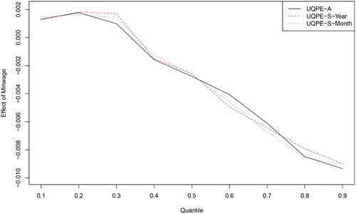
Next, we consider the proposed method UQPE-S in Sections 4. Since the data of minimum wage is recorded in years and the data of CPS is recorded in months, we consider b = 10 (year) and 120 (month), respectively. The data of 2011 and January 2011 are regarded as ${\mathit{D}}_1$ for UQPE-S-Year (b = 10) and UQPE-S-Month (b = 120), respectively. The difference between the estimated effect of Minwage for UQPE-A, UQPE-S-Year and UQPE-S-Month is illustrated in Figure 2, which plots at nine different quantiles (from the 10th to the 90th). From Table 7 and Figure 2, we can see that the estimated coefficients and the effects of Minwage on log wages under different quantiles by UQPE-A, UQPE-S-Year, and UQPE-S-Month are all very close.

Fig. 2 The estimates of the effect of Minwage on log wages by UQPE-A, UQPE-S-Year, and UQPE-S-Month for Labor income and minimum wage dataset.

Finally, as with the streaming data setup, when the last batch of data arrives (2020 and December 2020 are regarded as ${\mathit{D}}_b$ for UQPE-S-Year (b = 10) and UQPE-S-Month (b = 120), respectively), the total running time of UQPE-A with nine quantiles is also 52.98 sec, which needs to compute all the data. However, UQPE-S-Year is 0.87 sec and UQPE-S-Month is 0.08 sec, because only ${\mathit{D}}_b$ and some past statistics are required. In addition, for the setting of massive data, that is, all data can be stored, the cumulative time from 1 to b of UQPE-S-Year (b = 10) and UQPE-S-Month (b = 120) with nine quantiles is 21.58 sec and 18.51 sec, respectively. Therefore, UQPE-S (UQPE-S-Year and UQPE-S-Month) is much faster to compute than UQPE-A.

6.2 Daily Return of Stocks and Exchange Rate Dataset

In order to illustrate the proposed methods in Sections 4 for large batches b, we used data from 871 trading days between January 1, 2020 and August 25, 2023 for all companies listed on the Shanghai Stock Exchange in China and exchange rate between the U.S. dollar and the Chinese currency. The dataset contains 1,339,591 observations, where suspension and special treatment stock transactions have been deleted. There were 1546 stocks in 2020, 1629 stocks in 2021, 1665 stocks in 2022 and 1689 stocks in 2023. We focus on the effects of Return (daily return of stock) on the quantile of the unconditional distribution of ERF (exchange rate fluctuation).

In this application, $\mathit{Y}=\mathit{Return}$, which is (closing price of the day–closing price of the previous day)/closing price of the previous day, ${\mathit{X}}_1=\mathit{ERF}$, which is our interested covariate, ${\mathit{X}}_2=TR$ (daily turnover rate of stock) and ${\mathit{X}}_3=\mathit{Vol}$ (daily trading volume of stock). Similar to the analysis of streaming time series data conducted in Deshpande, Javanmard, and Mehrabi (2023) and Jiang, Choy, and Yu (2023), the dataset in this study is not independent and identically distributed. However, we employ OLS, UQPE-A, CQR, and UQPE-S to analyze the dataset. It is important to note that this application poses a limitation on the iid assumption commonly used in practical time series data analysis. Table 8 and Figure 3 report the estimated coefficients ${\mathit{X}}_1=\mathit{ERF}$ of model (6.1) with $\mathit{X}={({\mathit{X}}_1,{\mathit{X}}_2,{\mathit{X}}_3)}^{\top }$ by methods OLS, CQR, UQPE-A, and UQPE-S under nine different quantiles (from the 10th to the 90th), which shows the difference between conditional and unconditional quantiles regressions.

Fig. 3 The estimates of the effect of ERF on Return by OLS, CQR, UQPE-A, and UQPE-S.

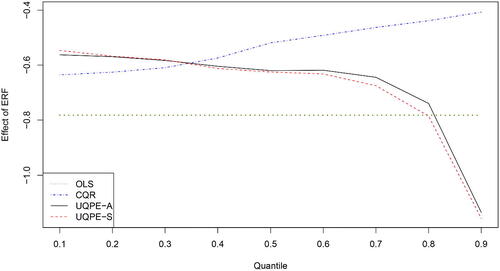
Table 8 The estimated coefficient of ERF by methods CQR, UQPE-A, and UQPE-S for Daily return of stocks and exchange rate dataset.

Method	$\tau =0.1$	0.2	0.3	0.4	0.5	0.6	0.7	0.8	0.9
CQR	−0.6335	−0.6257	−0.6094	−0.5740	−0.5190	−0.4916	−0.4628	−0.4384	−0.4071
UQPE-A	−0.5625	−0.5693	−0.5930	−0.6043	−0.6201	−0.6187	−0.6443	−0.7395	−1.1355
UQPE-S	−0.5466	−0.5674	−0.5812	−0.6121	−0.6252	−0.6322	−0.6749	−0.7856	−1.1572

Next, we consider the proposed method UQPE-S in Sections 4. For different stocks, the exchange rate is the same every day, so we choose ${\mathit{D}}_1$ for the first 30 trading days. Since the data between January 1, 2021 and August 25, 2023 is recorded in days, we consider b = 842. The difference between the estimated effect of ERF for UQPE-A and UQPE-S is illustrated in Table 8 and Figure 3. From Table 8 and Figure 3, we can see that the effects of ERF on Return under different quantiles by UQPE-A and UQPE-S are all very close.

Finally, as with the streaming data setup, when the last batch of data arrives (the transaction data as of August 25, 2023 is regarded as ${\mathit{D}}_b$), the total running time of UQPE-A with nine quantiles is also 65.37 sec and UQPE-S is 0.02 sec. In addition, for the setting of massive data, that is, all data can be stored, the cumulative time from 1 to b of UQPE-S (b = 842) with nine quantiles is 18.11 sec. Therefore, UQPE-S is much faster to compute than UQPE-A.

7 Discussion

In this article, we delve into renewable parameter estimation for unconditional quantile regression applied to streaming datasets. A pivotal insight derived from our work is the introduction of a smoothing logistic regression estimator, a crucial tool in generating renewable estimators for unconditional quantile regression. This innovative approach necessitates only the availability of the current data batch within the stream, along with sufficient statistics on the historical data at each stage of analysis. Notably, our proposed renewable methods do not impose constraints on the number of batches, allowing them to adapt seamlessly to situations where streaming data arrives rapidly and continuously.

Theoretical analysis reveals that the proposed estimators for streaming datasets attain optimal efficiency, with asymptotic covariance matrices mirroring those of estimators derived from full data. The algorithm’s swiftness stems from its reliance on the Newton-Raphson method. Empirical results presented in Sections 5 and 6 demonstrate that our proposed method closely approximates the estimator derived from complete data, yet boasts a shorter running time.

Furthermore, the smoothing technique employed for the logistic regression estimator in this article can be extended to benefit other estimation methods, such as quantile regression and Huber estimation. As highlighted in Kong and Xia (2019) and Jiang and Yu (2022), our renewable estimation method is not confined solely to streaming data, but is also apt for the analysis of massive data. “Massive data” denotes data that exceeds a computer’s storage or computational capacity, often originating from a distributed system. Specifically, we can employ the divide-and-conquer method to partition the dataset into b blocks, or the dataset itself may stem from b sub-devices. This empowers us to analyze massive data with the aid of our renewable estimation method.

Supplementary Materials

The proofs of the proposed theorems are given in the supplementary material file.

Acknowledgments

We thank the editor, associate editor and two reviewers for their constructive comments, which helped us improve the article.

Disclosure Statement

No potential conflict of interest was reported by the author(s).

Additional information

Funding

This research is supported by the National Social Science Foundation of China (Series number: 21BTU040) and the Ministry of Education of the People’s Republic of China, Humanities and Social Science Foundation (Series number: 22YJC910005) and London Mathematics Society (Scheme 42206).

References

- Amba, S. M., and Nguyen, B. H. (2019), “Exchange Rate and Equity Price Relationship: Empirical Evidence from Mexican and Canadian Markets,” The International Journal of Business and Finance Research, 13, 33–43.
- Bahmani-Oskooee, M., and Sohrabian, A. (1992), “Stock Prices and the Effective Exchange Rate of the Dollar,” Applied Economics, 24, 459–64. DOI: 10.1080/00036849200000020.
- Borgen, N. (2016), “Fixed Effects in Unconditional Quantile Regression,” The Stata Journal, 16, 403–415. DOI: 10.1177/1536867X1601600208.
- Chen, X., Liu, W., and Zhang, Y. (2019), “Quantile Regression Under Memory Constraint,” Annals of Statistics, 47, 3244–3273.
- Deshpande, Y., Javanmard, A., and Mehrabi, M. (2023), “Online Debiasing for Adaptively Collected High-Dimensional Data with Applications to Time Series Analysis,” Journal of the American Statistical Association, 118, 1126–1139. DOI: 10.1080/01621459.2021.1979011.
- Dube, A. (2019), “Minimum Wages and the Distribution of Family Incomes,” American Economic Journal: Applied Economics, 11, 268–304. DOI: 10.1257/app.20170085.
- Fernandes, M., Guerre, E., and Horta, E. (2021), “Smoothing Quantile Regressions,” Journal of Business & Economic Statistics, 39, 338–357. DOI: 10.1080/07350015.2019.1660177.
- Firpo, S., Fortin, N. M., and Lemieux, T. (2009), “Unconditional Quantile Regressions,” Econometrica, 77, 953–973.
- Ghosh, P. (2021), “Box-Cox Power Transformation Unconditional Quantile Regressions with An Application on Wage Inequality,” Journal of Applied Statistics, 48, 3086–3101. DOI: 10.1080/02664763.2020.1795817.
- He, X., Pan, X., Tan, K. M., and Zhou, W. (2023), “Smoothed Quantile Regression with Large Scale Inference,” Journal of Econometrics, 232, 367–388. DOI: 10.1016/j.jeconom.2021.07.010.
- Horowitz, J. (1998), “Bootstrap Methods for Median Regression Models,” Econometrica, 66, 1327–1352. DOI: 10.2307/2999619.
- Inoue, A., Li, T., and Xu, Q. (2021), “Two Sample Unconditional Quantile Effect,” arXiv:2105.09445v1.
- Jiang, R., Choy, S. K., and Yu, K. (2023), “Non-Crossing Quantile Double-Autoregression for the Analysis of Streaming Time Series Data,” Journal of Time Series Analysis. DOI: 10.1111/jtsa.12725.
- Jiang, R., and Yu, K. (2021), “Smoothing Quantile Regression for a Distributed System,” Neurocomputing, 466, 311–326. DOI: 10.1016/j.neucom.2021.08.101.
- ——(2022), “Renewable Quantile Regression for Streaming Data Sets,” Neurocomputing, 508, 208–224.
- ——(2023), “No-Crossing Single-Index Quantile Regression Curve Estimation,” Journal of Business & Economic Statistics, 41, 309–320.
- Koenker, R., and Bassett, G. (1978), “Regression Quantile,” Econometrica, 46, 33–50. DOI: 10.2307/1913643.
- Kong, E., and Xia, Y. (2019), “On the Efficiency of Online Approach to Nonparametric Smoothing of Big Data,” Statistica Sinica, 29, 185–201. DOI: 10.5705/ss.202015.0365.
- Lee, D. S. (1999), “Wage Inequality in the United States during the 1980s: Rising Dispersion or Falling Minimum Wage?” The Quarterly Journal of Economics, 114, 977–1023. DOI: 10.1162/003355399556197.
- Luo, L., and Song, P. (2020), “Renewable Estimation and Incremental Inference in Generalized Linear Models with Streaming Data Sets,” Journal of the Royal Statistical Society, Series B, 82, 69–97. DOI: 10.1111/rssb.12352.
- Luo, L., Zhou, L., and Song, P. (2023), “Real-Time Regression Analysis of Streaming Clustered Data with Possible Abnormal Data Batches,” Journal of the American Statistical Association, 118, 2029–2044. DOI: 10.1080/01621459.2022.2026778.
- Martinez-Iriarte, J., Montes-Rojas, G., and Sun, Y. (2022), “Location-Scale and Compensated Effects in Unconditional Quantile Regressions,” arXiv:2201.02292v1.
- Nadaraya, E. (1964), “Some New Estimates for Distribution Functions,” Theory of Probability and Its Applications, 9, 497–500. DOI: 10.1137/1109069.
- Pan, M.-S., Fok, R., and Liu, Y. (2007), “Dynamic Linkages between Exchange Rates and Stock Prices: Evidence from East Asian Markets,” International Review of Economics & Finance, 16, 503–520. DOI: 10.1016/j.iref.2005.09.003.
- Sasaki, Y., Ura, T., and Zhang, Y. (2022), “Unconditional Quantile Regression with High-Dimensional Data,” Quantitative Economics, 13, 955–978. DOI: 10.3982/QE1896.
- Schifano, E., Wu, J., Wang, C., Yan, J., and Chen, M.-H. (2016), “Online Updating of Statistical Inference in the Big Data Setting,” Technometrics, 58, 393–403. DOI: 10.1080/00401706.2016.1142900.
- Wang, H., Min, Y., and Stufken, J. (2019), “Information-based Optimal Subdata Selection for Big Data Linear Regression,” Journal of the American Statistical Association, 114, 393–405. DOI: 10.1080/01621459.2017.1408468.
- Wang, K., Wang, H., and Li, S. (2022), “Renewable Quantile Regression for Streaming Datasets,” Knowledge-Based Systems, 235, 107675. DOI: 10.1016/j.knosys.2021.107675.
- Xie, R., Bai, S. Y., and Ma, P. (2023), “Optimal Sampling Designs for Multi-Dimensional Streaming Time Series with Application to Power Grid Sensor Data,” arXiv:2303.08242v1.
- Yang, Y., and Yao, F. (2023), “Online Estimation for Functional Data,” Journal of the American Statistical Association, 118, 1630–1644.
- Zhang, B., and Li, X. (2010), “Currency Appreciation and Stock Market Performance: Evidence from China,” Frontiers of Economics in China, 5, 393–411. DOI: 10.1007/s11459-010-0104-2.