Investigating Growth-at-Risk Using a Multicountry Nonparametric Quantile Factor Model

Abstract

We develop a nonparametric quantile panel regression model. Within each quantile, the quantile function is a combination of linear and nonlinear parts, which we approximate using Bayesian Additive Regression Trees (BART). Cross-sectional information is captured through a conditionally heteroscedastic latent factor. The nonparametric feature enhances flexibility, while the panel feature increases the number of observations in the tails. We develop Bayesian methods for inference and apply several versions of the model to study growth-at-risk dynamics in a panel of 11 advanced economies. Our framework usually improves upon single-country quantile models in recursive growth forecast comparisons.

Keywords:

• Macroeconomic forecasting
• Nonparametric regression
• Regression trees
• Spillovers

1 Introduction

Empirical macroeconomics has seen an upsurge of interest in modeling the tails of predictive distributions. A recent influential paper is Adrian, Boyarchenko, and Giannone (ABG, 2019), which investigated the impact of financial conditions on the conditional distribution of GDP growth and found it to be important in the lower quantiles. Before and after ABG, a large literature has used quantile regression methods to forecast tail risks to economic growth (see, among many others, Giglio, Kelly, and Pruitt 2016; De Nicolò and Lucchetta 2017; Cook and Doh 2019; González-Rivera, Maldonado, and Ruiz 2019; Delle Monache, De Polis, and Petrella 2020; Figueres and Jarociński 2020; Plagborg-Møller et al. 2020; Reichlin, Ricco, and Hasenzagl 2020; Adrian et al. 2022; Ferrara, Mogliani, and Sahuc 2022; Mitchell, Poon, and Mazzi 2022). Other studies consider tail risks to other macroeconomic variables such as unemployment or inflation (e.g., Gaglianone and Lima 2012; Manzan and Zerom 2013; Manzan 2015; Korobilis 2017; Ghysels, Iania, and Striaukas 2018; Galbraith and van Norden 2019; Korobilis et al. 2021; Kiley 2022; Pfarrhofer 2022).

The existing literature, with few exceptions, uses quantile models for a single variable of interest. These models assume a linear relationship between the predictors and the quantile function of some outcome variable.¹ For macroeconomic data this assumption might be warranted in normal times but in turbulent times it could be that relationships change or turn nonlinear. Moreover, often several variables rather than a single one are of interest, so that a joint model would be preferable. These observations motivate the model we develop in this article.

In contrast to much of the existing literature we propose a nonparametric model which involves multiple equations and allows for the assessment of whether the quantile function is linear or unknown and possibly highly nonlinear. In particular, the model we propose is a multicountry, nonparametric quantile regression, which we then use to investigate growth-at-risk in a panel of 11 advanced economies.

The justification for adopting nonparametric methods is provided by Clark et al. (2023) and Huber et al. (2023), which find Bayesian nonparametric vector autoregressions (VARs) to be able to successfully model the tails of predictive densities of macroeconomic variables in a flexible and accurate manner. These papers found that Bayesian Additive Regression Trees (BART) are an effective nonparametric method that is particularly useful in crisis times (e.g., the Financial Crisis of 2008/2009 or the Covid pandemic) when growth-at-risk issues are of particular importance. However, in normal periods, the predictive gains from using BART are more muted (and sometimes negative). In this article we extend the BART regression methods used in these papers to the quantile BART case. Since the predictive gains of BART vary over the business cycle, we assume that within each quantile, the quantile function is the sum of a linear model and some unknown nonlinear function, which we approximate using BART. Studies such as Taddy and Kottas (2010) have developed other Bayesian approaches to nonparametric model-based quantile regression.

The justification for use of a multicountry model is that a panel dimension can often improve forecasts with respect to single-country models; see, among many others, Bai et al. (2022) and Feldkircher et al. (2022). Moreover, and specifically for the quantile case, macroeconomic datasets are short, leading to a small number of observations in the tails of the distribution. We develop a model for the pth quantile that includes a factor that summarizes the available cross-country information at that quantile. In addition, as indicated below, our Bayesian model specification has features that allow information from other countries to inform estimates for a given country. Exploiting this cross-country information through a pooling prior may improve predictive accuracy by parsimoniously including international information to inform coefficients associated with domestic quantities.

In terms of empirical results, our proposed models commonly improve on the benchmark single-country parametric quantile model in recursive growth forecast comparisons, more so in the tails than near the center of the distribution. Importantly, we find that combining BART with quantile regressions pays off in terms of predictive accuracy, especially in the right tail. Moreover, some form of international information (either by directly including non-domestic series or through the introduction of the static heteroscedastic factor) leads to accuracy gains. Zooming into U.S.-specific results reveals nonlinear effects of financial conditions on growth-at-risk whereas the effects are closer to a linear specification when moving toward the center of the distribution. This is corroborated by a higher relevance (in terms of variation explained) of the BART piece.

Focusing on full sample results suggests that the common factor is important. It explains a large fraction of the forecast error variance in most countries and during most time periods (with particularly high shares during recessionary episodes).

The remainder of the article is structured as follows. Section 2 defines and motivates our QF-BART model, including the relevant priors, and provides additional details on how we compute predictions. Section 3 contains the forecast evaluation. Section 4 considers international growth-at-risk dynamics. Section 5 summarizes and concludes.

2 A Multicountry Nonparametric Quantile Factor Model

We model the joint distribution of (for simplicity, de-meaned) output growth for a panel of N countries. These are stored in an N-dimensional vector ${\mathit{y}}_t=(y_{1,t},\dots ,y_{N,t})\prime$ with $y_{i,t}$ denoting time t output growth in country i. Domestic real activity might depend on the lags of ${\mathit{y}}_t$ as well as lags of other exogenous factors, both of which are included in a K-dimensional vector ${\mathit{x}}_{i,t}$. We adopt a notational convention where ${\mathit{x}}_{i,t}$ is structured such that J domestic quantities for country i are always ordered first, followed by all K – J non-domestic variables if applicable (i.e., lagged output growth rates of the other countries). We assume that $y_{i,t} (i=1,\dots ,N)$ follows a quantile regression model which, for the pth quantile, is given by: (1) $$y_{i,t}={\omega }_g{g}_{\mathit{\text{ip}}}({\mathit{x}}_{i,t})+{\omega }_{\beta }\mathit{\beta }{\prime }_{\mathit{\text{ip}}}{\mathit{x}}_{i,t}+{\lambda }_{\mathit{\text{ip}}}{f}_{p,t}+{ϵ}_{\mathit{\text{ip}},t},\hspace{1em}{ϵ}_{\mathit{\text{ip}},t}\sim {\text{AL}}_p({\sigma }_{\mathit{\text{ip}}}),$$(1) with $g_{\mathit{\text{ip}}}:{\mathbb{R}}^K\to \mathbb{R}$ denoting unknown country-specific functions and ${\mathit{\beta }}_{\mathit{\text{ip}}}$a $K\times 1$-dimensional vector of regression coefficients; ω_g and ${\omega }_{\beta }$ are deterministic binary parameters that we use to select the parametric or nonparametric part, or both parts of our model, respectively. The case ${\omega }_g=1$ and ${\omega }_{\beta }=0$ would correspond to a fully nonlinear model (labeled BART), whereas ${\omega }_g=0$ and ${\omega }_{\beta }=1$ would be a (conditionally) linear quantile regression (QR). Setting ${\omega }_g={\omega }_{\beta }=1$ yields a model which estimates both linear and nonparametric parts, which we refer to as mixBART (see also Clark et al. 2023).

Shocks to domestic economic conditions often feature cross-sectional dependence. Kose, Otrok, and Whiteman (2003) show that business cycles in a large panel of economies feature a factor structure and tend to co-move. Similarly, Stock and Watson (2005) find that a significant portion of the widespread reduction in the volatility of G7 economic activity is associated with a reduction in the magnitude of the common international shocks. In our model, we introduce a common shock term to capture contemporaneous relations across the elements in ${\mathit{y}}_t$. This leads to a static factor model with ${\lambda }_{\mathit{\text{ip}}}$ denoting the country-specific factor loading and $f_{p,t}$ the corresponding international factor. Both the factors and factor loadings are quantile-specific. We assume that the latent factor is conditionally independent over time and arises from a Gaussian distribution, $f_{p,t}|h_{p,t}\sim \mathcal{N}(0,\hspace{0.17em}\mathrm{\text{exp}}\hspace{0.17em}(h_{p,t}))$, with $h_{p,t}$ being a (logarithmic) variance that evolves according to an AR(1) process: $$h_{p,t}={\mu }_p+{\rho }_p(h_{p,t-1}-{\mu }_p)+{\varsigma }_p{u}_{p,t},\hspace{1em}{u}_{p,t}\sim \mathcal{N}(0,1).$$

Here we let μ_p denote the unconditional mean, ρ_p the autoregressive parameter, and ${\varsigma }_p^2$ the error variance of the log-volatility process. This log-volatility process introduces dependence over time.

The presence of the factor implies that the equations across countries but within a given quantile are correlated. Using the jargon from the panel VAR literature (see Canova and Ciccarelli 2013), the factor establishes static interdependencies across countries. An economic interpretation of the factor, related to the findings in Stock and Watson (2005), is that it reflects a common international business cycle shock that affects the pth quantile function of each country. The Online Appendix provides additional details on the interpretation and implications of the factor structure.

Finally, ${ϵ}_{\mathit{\text{ip}},t}$ follows an asymmetric Laplace (AL) distribution scaled by a parameter σ_ip with its pth quantile being equal to zero. The AL distribution is chosen purely as a technical device to target the pth quantile of the dependent variable in order to estimate the underlying quantile function.²

2.1 Discussion of Model Features

The model proposed in the previous section possesses several features which should not only improve its predictive capabilities but also allow for additional inferential opportunities. Here, we briefly summarize these features.

First, the flexible combination of linear and nonparametric components allows for capturing different degrees of nonlinearities across quantiles. The recent literature finds that macroeconomic relations differ in the lower tails of the distribution of output growth compared to the middle of the distribution and upper tails, as well as that, in the the lower tails, macroeconomic relations might be subject to substantial nonlinearities. The former observation on relationships changing in the lower tails relates to the fact that coefficients of a regression model can change during extreme periods and can be well captured with a linear QR (see, e.g., ABG). The latter observation concerns additional nonlinearities in the effects of selected covariates on output growth that may occur in a given quantile. These nonlinearities could change across quantiles, perhaps being more important in the extremes of a distribution and relatively unimportant in tranquil periods of the business cycle (e.g., in the center of the distribution). BART provides enough flexibility to capture these nonlinearities that may exist across and within quantiles of the data generating process (DGP).

Second, our model allows for lagged and contemporaneous relations across countries. The key point to notice is that these interdependencies can differ across quantiles. For instance, it could be that in the presence of a global adverse economic shock, cross-country dependencies are more important than during tranquil times. This behavior is effectively captured by estimating separate loadings, factors, functions g_ip , and regression parameters ${\mathit{\beta }}_{\mathit{\text{ip}}}$. For instance, in normal periods it could be that short-run fluctuations in GDP growth depart from each other. In such a situation, the corresponding factor loadings ${\mathit{\lambda }}_p=({\lambda }_{1p},\dots ,{\lambda }_{\mathit{\text{Np}}})\prime$ should be close to zero for p close to the median.

Third, since the factor is conditionally heteroscedastic, it can also control for sudden common shifts in the conditional variance of the dependent variables. Inclusion of this factor allows us to control for shocks common to all countries in our panel, a feature which might be extremely important during periods such as the recent Covid pandemic (see, e.g., the discussion in Carriero et al. (in-press)). In addition, the fact that the volatility process evolves according to an AR(1) process implies that the factor displays no time dependence conditional on $h_{p,t}$ but might be persistent after integrating out $h_{p,t}$.

2.2 Approximating the Unknown Functions Using BART

We treat the function g_ip as unknown and approximate it using BART (Chipman, George, and McCulloch 2010). Though other alternatives are possible, BART has been successfully employed in economics for forecasting financial time series in Huber and Rossini (2022), nowcasting GDP in selected European economies in Huber et al. (2023), and tail forecasting of output, inflation, and unemployment in Clark et al. (2023). BART is a sum-of-trees model that approximates g_ip by summing over many individual trees that all take a simple form and act as “weak learners.”

The BART approximation for g_ip is given by: $$g_{\mathit{\text{ip}}}\approx {\widehat{g}}_{\mathit{\text{ip}}}=\sum _{s=1}^{S}v({\mathit{x}}_{i,t}|{\mathcal{T}}_{\mathit{\text{ip}}}^s,{\mathit{\mu }}_{\mathit{\text{ip}}}^s),$$ with v denoting a tree function that is determined by a tree structure ${\mathcal{T}}_{\mathit{\text{ip}}}^s$ and a vector of terminal node parameters ${\mathit{\mu }}_{\mathit{\text{ip}}}^s$. This terminal node parameter vector has dimension $b_{\mathit{\text{ip}}}^s$ and is country (i), quantile (p) and tree (s) specific.

The tree structure consists of multiple binary decision rules that ask whether a covariate exceeds a threshold and, according to them, produces (disjoint) partitions of the input space. These take the form $x_{\mathit{\text{ij}},t}>c$ or $x_{\mathit{\text{ij}},t}\le c$, with $x_{\mathit{\text{ij}},t}$ denoting the jth element of ${\mathit{x}}_{i,t}$ and c being a splitting/threshold value. Sequences of these decision rules lead to a terminal node coupled with a corresponding terminal node parameter in ${\mathit{\mu }}_{\mathit{\text{ip}}}^s$. The parameters in ${\mathit{\mu }}_{\mathit{\text{ip}}}^s$ thus act as the “leaves” of the tree. That is, they are fitted values assigned to the observations which are allocated to a specific terminal node based on the splits determined by the configuration in ${\mathit{x}}_{i,t}$.

BART is capable of handling arbitrary forms of nonlinearities. For instance, it flexibly handles higher order interaction effects between the covariates and the responses, picks up time variation and, if necessary, also allows for linear relations.

When S is large, the BART approximation is prone to overfitting if no further regularization is introduced. Chipman, George, and McCulloch (2010) use regularization priors to force the trees to be simple. We achieve this through shrinkage priors on the tree structure and the terminal node parameters. Following Chipman, George, and McCulloch (1998), the prior on ${\mathcal{T}}_{\mathit{\text{ip}}}^s$ is obtained by constructing a tree-generating stochastic process. The prior $p({\mathcal{T}}_{\mathit{\text{ip}}}^s)$ has three key aspects. First, tree complexity ultimately depends on the depth of the tree. Since the tree-generating process grows trees sequentially, we let d denote the current depth of the tree. Hence, if d is large, the tree is complex and thus might overfit the data. To force the individual trees to be simple, we assume that a given node at depth d is nonterminal with probability proportional to $\alpha {(1+d)}^{-\zeta },$ where α is between 0 and 1 and $\zeta >0$. Notice that this probability decreases in d which implies that growing more complicated trees becomes unlikely if d is large. The amount of shrinkage is controlled by α and ζ. These hyperparameters are often set to $\alpha =0.95$ and ζ = 2, implying that trees with two or three terminal nodes receive over 80% of total prior probability. Chipman, George, and McCulloch (2010) found that, for over 40 datasets, this choice performs well, and extensive cross-validation for α and ζ only improves predictive accuracy by small margins. The second and third aspects of the prior are concerned with how decision rules are constructed. To this end, we use discrete uniformly distributed priors to select the variables showing up in the decision rule as well as a uniform prior over the splitting/threshold values.

The second source of shrinkage is a Gaussian shrinkage prior on ${\mu }_{\mathit{\text{ij}},p}^s$, the jth element of ${\mathit{\mu }}_{\mathit{\text{ip}}}^s$. Chipman, George, and McCulloch (2010) recommend scaling the prior using the range of the data. More specifically, let $y_{i,\mathrm{\text{min}}}$ and $y_{i,\mathrm{\text{max}}}$ denote the minimum and maximum of the observed data in country i. The corresponding Gaussian prior is then ${\mu }_{\mathit{\text{ij}},p}^s\sim \mathcal{N}(0,v_{\mathit{\text{ip}}}^2)$, setting $v_{\mathit{\text{ip}}}=(y_{i,\mathrm{\text{max}}}-y_{i,\mathrm{\text{min}}})/\left(2\gamma \sqrt{S}\right)$ with $\gamma >0$ being a prior scaling parameter, typically set equal to 2. The prior implies that if the number of trees S is large, the prior variance decreases and the amount explained by a single tree is decreased; in line with the related literature, we set S = 250. This is consistent with each tree explaining only a small share of variation in the response variable, but the ensemble model provides sufficient flexibility to capture even complicated conditional mean relations. Another feature, noted by Huber et al. (2023), is that the prior variance increases in the range of the data. Hence, if outliers arise, the prior becomes increasingly loose and allows for more flexibility in terms of prior probability about capturing observations outside the range of past data.

The priors on the tree structures and the terminal node parameters constitute the main ingredients of BART. Since our model also features a linear part, we also need to specify priors on ${\mathit{\beta }}_{\mathit{\text{ip}}}$, which are discussed in the next section.

2.3 Priors on the Remaining Coefficients of the Model

On the coefficients ${\mathit{\beta }}_{\mathit{\text{ip}}}$ we use a variant of the horseshoe prior: ${\beta }_{\mathit{\text{ij}},p}\sim \mathcal{N}({\underset{¯}{\beta }}_{\mathit{\text{jp}}},{\phi }^2{\psi }_{\mathit{\text{ij}},p}^2)$ with scaling parameters $\phi \sim {\mathcal{C}}^{+}(0,1)$ and ${\psi }_{\mathit{\text{ij}},p}\sim {\mathcal{C}}^{+}(0,1)$; ${\mathcal{C}}^{+}$ denotes a half-Cauchy distribution, ${\psi }_{\mathit{\text{ij}},p}$ is a coefficient and quantile-specific scaling parameter, and $\phi$ is a global shrinkage parameter that is common to all coefficients. Notice that the presence of $\phi$ introduces dependencies across coefficients (including across countries) and across quantiles. The key advantage is that the presence of the local shrinkage parameters ${\psi }_{\mathit{\text{ij}},p}$ allows the detection of signals (i.e., nonzero or heterogeneous ${\beta }_{\mathit{\text{ij}},p}$ over the cross section) even if $\phi$ is close to zero.

The prior mean ${\underset{¯}{\beta }}_{\mathit{\text{jp}}}$ pools information over the cross section. In our hierarchical specification, it is estimated from the data using a Gaussian prior for the domestic variables, and deterministically set to zero for non-domestic quantities: ${\underset{¯}{\beta }}_{\mathit{\text{jp}}}\sim \mathcal{N}(0,{\tilde{\phi }}_j)$ for $j=1,\dots ,J,$ with ${\underset{¯}{\beta }}_{\mathit{\text{jp}}}=0$ for $j=J+1,\dots ,K$. The parameter ${\tilde{\phi }}_j$ is the prior variance of the common mean, which we set to a weakly informative value of 10 for the empirical application. We refer to this prior as the pooled horseshoe (HSP).³

For the factor loadings λ_ip , we use a set of independent Gaussian priors for all i, p: ${\lambda }_{\mathit{\text{ip}}}\sim \mathcal{N}(0,1)$. Note that λ_ip is a scalar and, hence, we use this relatively weakly informative prior rather than a prior such as the HS which is used to avoid over-parameterization as might occur with high dimensional parameters.

The remaining coefficients of the model relate to the error term. Kozumi and Kobayashi (2011) write the AL using a scale-location mixture of Gaussians: (2) $${ϵ}_{\mathit{\text{ip}},t}={\theta }_p{\nu }_{\mathit{\text{ip}},t}+{\tau }_p\sqrt{{\sigma }_{\mathit{\text{ip}}}{\nu }_{\mathit{\text{ip}},t}}{e}_{\mathit{\text{ip}},t},$$(2) with ${\theta }_p=\frac{1-2p}{p(1-p)},\hspace{1em}{\tau }_p^2=\frac{2}{p(1-p)},\hspace{1em}{\nu }_{\mathit{\text{ip}},t}={\sigma }_{\mathit{\text{ip}}}{z}_{\mathit{\text{ip}},t},\hspace{1em}{e}_{\mathit{\text{ip}},t}\sim \mathcal{N}(0,1)$, and $z_{\mathit{\text{ip}},t}\sim \hspace{0.17em}\mathrm{\text{Exp}}\hspace{0.17em}(1)$.⁴ On the scale parameter σ_ip we use an inverse Gamma prior, ${\sigma }_{\mathit{\text{ip}}}\sim {\mathcal{G}}^{-1}(a_{\sigma }/2,b_{\sigma }/2),$ with the relatively weakly informative choices of $a_{\sigma }=1$ and $b_{\sigma }=1$. This completes the prior setup. Details of the Markov chain Monte Carlo (MCMC) algorithm used to carry out posterior inference are provided in the Online Appendix.

2.4 Remarks on Computing Predictive Distributions

Our focus is on predicting international GDP growth up to h-steps-ahead where $h\ge 1$. In Section A.2 of the Online Appendix we provide a detailed account on how to compute these predictive densities. Here, we give a brief summary and focus on the difficulties in computing predictive densities in nonparametric quantile regressions. As detailed in (A.1) of the Online Appendix, the predictive distribution for the pth quantile of h-step-ahead GDP growth in country i, (3) $$\begin{array}{c}p({\mathcal{Q}}_p(y_{i,T+h})|{\mathit{y}}_{1:T},{\mathit{x}}_{1:T},{\mathit{x}}_{i,T+h})\\ \mathrm{\hspace{1em}}\mathrm{\hspace{1em}}={\int }_{{\mathbf{\Xi }}_{\mathit{p}}}p({\mathcal{Q}}_p(y_{i,T+h})|{\mathbf{\Xi }}_{\mathit{p}},{\mathit{x}}_{i,T+h})p({\mathbf{\Xi }}_{\mathit{p}}|{\mathit{y}}_{1:T},{\mathit{x}}_{1:T})d{\mathbf{\Xi }}_{\mathit{p}},\end{array}$$(3) is obtained through Monte Carlo integration by sampling from the posterior of the parameters and the latent states, stored in ${\mathbf{\Xi }}_{\mathit{p}}$, and then computing the forecast of the pth quantile ${\mathcal{Q}}_p(y_{i,T+h})$. The first term on the right-hand side of (3) is the conditional predictive distribution that is Gaussian and depends on ${\mathit{x}}_{i,T+h}$ which includes only information that is available up to time T. Depending on the specification, ${\mathit{x}}_{i,T+h}$ includes GDP growth for all countries measured in time T and the CISS in time T. The second term is the posterior distribution with ${\mathit{y}}_{1:T}$ and ${\mathit{x}}_{1:T}$ denoting full data matrices that have typical rows $\mathit{y}{\prime }_t$ and $(\mathit{x}{\prime }_{1,t},\dots ,\mathit{x}{\prime }_{N,t})$.

Two remarks are in order about (3). First, computing (3) over a grid of quantiles p provides information that can be used to back out the predictive distribution implied by the different quantiles of our model. This, however, relies on approximations to the true predictive density. For instance, Adrian, Boyarchenko, and Giannone (2019) estimate the predictive quantiles and then fit a skew-t distribution to approximate the exact predictive density. In our framework, we use the posterior median of the predictive quantiles to back out the full predictive distribution nonparametrically using the methods outlined in Mitchell, Poon, and Zhu (2023). This is necessary if interest is on computing functions of forecasts such as average forecasts over different horizons, probabilistic forecasts or risk measures based on forecast distributions.

Second, for h > 1 we face the issue of whether we use direct or iterative forecasts. Since ${\mathit{x}}_{i,t}$ includes exogenous quantities, computing iterative forecasts requires making assumptions on how the exogenous elements in ${\mathit{x}}_{i,t}$ evolve over the forecast horizon. Moreover, as Marcellino, Stock, and Watson (2006) show, the predictive accuracy of iterative forecasts might be more affected by model mis-specification. This risk is lessened through the use of direct forecasts, the approach we adopt. Direct forecasts have the advantage that no assumptions on how the exogenous elements in ${\mathit{x}}_{i,t}$ evolve over time are required. In addition, one can compute them straightforwardly within our nonparametric and quantile-specific model.

One disadvantage, however, is that by computing direct forecasts we potentially neglect a nonlinear moving average structure in the shocks and this might impact predictive inference.⁵ To see this more clearly, let us consider a special case of our general model in (1) that sets ${\omega }_g=1$ and ${\omega }_{\beta }=0$ and ${\mathit{x}}_{i,t}=y_{i,t-1}$ (i.e., no exogenous quantities). The resulting one-step-ahead predictive regression is then given by $y_{i,t+1}=g_{\mathit{\text{ip}}}(y_{i,t})+r_{i,t+1}$, where $r_{i,t+h}={\lambda }_{\mathit{\text{ip}}}{f}_{p,t+h}+{ϵ}_{\mathit{\text{ip}},t+h}$. The two-step-ahead iterative forecasting equation is $y_{i,t+2}=g_{\mathit{\text{ip}}}(g_{\mathit{\text{ip}}}(y_{i,t})+r_{i,t+1})+r_{i,t+2}$ and thus depends on $r_{i,t+1}$. In general, for h-steps-ahead the relevant predictive equation reads: $$y_{i,t+h}={\tilde{g}}_{\mathit{\text{ip}}}^{(h)}(y_{i,t},r_{i,t+h-1},\dots ,r_{i,t+1})+r_{i,t+h},$$ where ${\tilde{g}}_{\mathit{\text{ip}}}^{(h)}$ is a composite function defined recursively. Instead, our direct forecasting approach implies the following approximation through a function ${\widehat{g}}_{\mathit{\text{ip}}}$: $${\tilde{g}}_{\mathit{\text{ip}}}^{(h)}(y_{i,t},r_{i,t+h-1},\dots ,r_{i,t+1})\approx {\widehat{g}}_{\mathit{\text{ip}}}^{(h)}(y_{i,t}),$$ where ${\widehat{g}}_{\mathit{\text{ip}}}^{(h)}(y_{i,t})$ denotes the BART estimate from the model $y_{i,t+h}={\widehat{g}}_{\mathit{\text{ip}}}^{(h)}(y_{i,t})+r_{i,t+h}$. Hence, the composite function ${\tilde{g}}^{(h)}$ might take an extremely complicated form and depends on the forecasts errors up to horizon h – 1, and is approximated, again, through BART. In contrast to linear models, we argue that the BART approximation is more robust to mis-specification related to (a neglect of) serial correlation in the factors and errors in the direct forecasting setup.⁶

In Online Appendix A.3 we carry out two robustness exercises to check whether the potential neglect of a moving average term is having an impact on our empirical findings. First, we augment our model to include estimates of forecast errors (see Lusompa 2023, for a discussion). Second, we use iterative forecasting methods (under a random walk assumption for the exogenous covariates in ${\mathit{x}}_{i,t}$). Both these approaches produce forecast scores which are almost identical to those produced in the main body of the article. We view this as evidence that our nonparametric model can flexibly adjust to mis-specification caused by approximating the composite function ${\tilde{g}}_{\mathit{\text{ip}}}^{(h)}(y_{i,t},r_{i,t+h-1},\dots ,r_{i,t+1})$ through ${\widehat{g}}_{\mathit{\text{ip}}}^{(h)}(y_{i,t})$ and by omitting the forecast errors.

3 Forecast Evaluation

3.1 Data, Competitors and Forecasting Design

Our sample runs from 1975Q1 to 2021Q4. We use real GDP data from the Main Economic Indicators (MEI) database, maintained by the OECD, and the composite indicator of systemic stress (CISS) by the European Central Bank. For data availability reasons we include Austria (AT), Denmark (DK), Finland (FI), France (FR), Germany (DE), Italy (IT), Netherlands (NL), Spain (ES), Sweden (SE), United Kingdom (UK), and the United States (US). This yields a cross-section of N = 11 countries. Charts of our dataset are provided in the Online Appendix.

The models are estimated for $p\in \{$0.05,0.1,0.16,0.25,0.4,0.5,0.6,0.75,0.84,0.9,0.95$\}$ and we forecast for $h=1,\dots ,4$. Our focus is on modeling the annualized quarterly growth rate of real GDP, measured as $y_{i,t}=400\times \hspace{0.17em}\mathrm{\text{log}}\hspace{0.17em}(Y_{i,t}/Y_{i,t-1})$, with $Y_{i,t}$ denoting real GDP in levels in time t. We denote the CISS for country i as $z_{i,t}$. For each model, we consider two different choices for the covariates. The first includes the lag of GDP growth and the CISS for country i in the equation for $y_{i,t}$, implying that K = 2, which we refer to as the single-country (SC) specification. The second contains cross-country information in ${\mathit{x}}_{i,t}$ by including the lag of GDP growth and the CISS of all countries jointly; hence, $K=2N$. This is referred to as CC to indicate that the information set includes cross-country data. In terms of (3), this specification implies that ${\mathit{x}}_{i,T+h}=(y_{1,T},z_{1,T},\dots ,y_{N,T},z_{N,T})\prime$ and $y_{i,T+h}=400\times \hspace{0.17em}\mathrm{\text{log}}\hspace{0.17em}(Y_{i,T+h}/Y_{i,T+h-1})$. In terms of the prior, we report results for our specification that allows for pooling through the prior HSP, as it generally performs a little better than the standard horseshoe prior that forces the coefficients to zero (the Online Appendix includes some comparisons).

All specifications we consider can be viewed as simpler variants of our general model. These simplifications relate to the dataset chosen (i.e., the SC or CC variant), whether the static factor is included, and whether we consider nonparametric quantile functions.

Then, we consider models that allow for static relations across countries within a given quantile. These models have a factor structure produced by allowing ${\mathit{\lambda }}_p\ne \mathbf{0}$. If we use a factor we add the label FM. Finally, we investigate whether BART-based models can improve tail forecasts by setting ${\omega }_{\beta }=0,{\omega }_g=1$. This yields the multicountry quantile BART model (labeled BART). The linear (Bayesian) quantile regression is obtained by excluding the nonparametric component by setting ${\omega }_{\beta }=1$, ${\omega }_g=0$. This model is labeled QR. Finally our most flexible model includes both linear and nonparametric components, with ${\omega }_{\beta }={\omega }_g=1$. This specification is labeled as mixBART. An overview of all models is provided in Table 1.

Table 1 Model overview.

Data	Weights	Factor
Single-country (SC)	${\omega }_g=0,{\omega }_{\beta }=1$ (QR)	${\mathit{\lambda }}_p=0$ (—)
Cross-country (CC)	${\omega }_g=1,{\omega }_{\beta }=0$ (BART)	${\mathit{\lambda }}_p\ne 0$ (FM)
	${\omega }_g={\omega }_{\beta }=1$ (mixBART)

NOTE: “Data” refers to the information set for individual country models. “Weights” refers to the specification of the conditional quantile function: parametric, nonparametric, or both parts. “Factor” indicates whether an international factor modeling the cross-sectional covariance structure within quantiles is present. We consider all possible combinations of these specification choices.

It is worth stressing that the different combinations above can also be used to end up with the benchmark specification proposed in ABG. This is achieved by including only the CISS and lagged GDP growth as covariates and excluding the factor and nonparametric components of the models. To ensure comparability to ABG, we estimate this benchmark using frequentist methods. The Bayesian version of ABG is obtained by removing the factor and setting ${\omega }_{\beta }=1,{\omega }_g=0$.

In the tables and figures that follow, we will use acronyms to indicate the different models. For doing so, we adopt the convention that we first indicate the model (i.e., whether we use QR, BART or mixBART), then (if applicable) whether we use the HSP prior, then whether cross-country information is included and finally whether we use a factor model or not. For instance, BART CC FM denotes the BART-based panel model with cross-country information and the factor being present.

After describing the data and models, we now briefly discuss the design of our forecasting exercise. We carry out recursive forecasting that is based on an expanding window of observations. As stressed in Section 2.4 we compute h > 1-step-ahead forecasts using the direct forecasting approach. The first 60 quarters of data are used as the initial estimation sample, which implies our forecast evaluation period begins in 1990Q1 for h = 1 and 1990Q4 for h = 4. We use the posterior median of the predictive quantiles.⁷ It is also worth noting that, for h = 4, ABG target the average annual growth rate, $400\times \hspace{0.17em}\mathrm{\text{log}}\hspace{0.17em}(Y_{i,T+h}/Y_{i,T})/h$, and we average our horizon-specific quarterly growth rate forecasts for $h=1,2,3,4$ to be in line with this target. To compute this average, we proceed as follows. We estimate the predictive quantiles for the h-step-ahead forecast and based on these infer the implied predictive distribution to obtain a smooth version from which we can readily sample future relations of $y_{i,T+h}$. This is achieved using the techniques outlined in Mitchell, Poon, and Zhu (2023) and yields horizon-specific smooth predictive densities which we then use to compute posterior distributions of average growth rate forecasts and the corresponding quantiles.⁸ More details are provided in the Online Appendix.⁹

After obtaining forecasts for the different quantiles, we evaluate predictive accuracy using Quantile Scores (QS) and quantile-weighted continuous ranked probability scores (qw-CRPS, see Gneiting and Ranjan (2011) and the Online Appendix) with three weighting schemes: no weighting, that is, conventional CRPS, labeled “none”; left tail, “left;” and right tail, “right.”

3.2 Tail Forecasting with Nonparametric Quantile Regressions

In this section we first discuss the overall forecasting performance for the different models and loss functions. Then, we focus on the best performing models and discuss differences in predictive accuracy across countries. Finally, we consider details about the forecasting properties of the model for US GDP growth, which has been the focus of a large previous literature, and for Italy and Sweden, as examples of countries for which BART works relatively well in the right and left tails, respectively.

3.2.1 Overall Results

Our forecasting exercise gives rise to a great deal of information. We consider a large number of models that differ along the dimensions outlined in the previous sub-section, and we obtain country-specific forecasting results. To first achieve an understanding about the predictive accuracy across countries, we focus on boxplots, shown in Figure 1. Each of these boxplots represents the cross-country dispersion of the different qw-CRPSs relative to the ABG benchmark of the various models. Blue lines are the median over the cross section, red lines show the mean and black points mark individual countries. The black vertical line is centered on unity, implying that if the mean (median) is located to the left of the vertical line, a given model outperforms the ABG benchmark on average across the countries under consideration (for at least 50% of the countries). These plots provide a simple means of assessing the overall performance of the models and whether forecast accuracy is heterogeneous across countries.

Fig. 1 Boxplots of relative quantile weighted continuous ranked probability scores (CRPS) for $h\in \{1,4\}$ benchmarked to the frequentist ABG model. Lower ratios indicate better performance. Blue lines are the median over the cross section, and red lines show the mean. Points indicate individual countries.

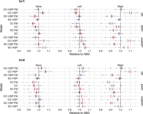
Figure 1 indicates that the overall best model in terms of average and median performance across countries, criteria and horizons is BART CC FM. QR CC-HSP FM is comparable only in the left tail for h = 1, and QR SC-HSP FM only in the right tail for h = 1 and h = 4.

About the importance of the cross country information, while results are mixed for QR and mixBART, for the best performing BART specification CC is better than SC in all cases and for both horizons. This finding is in line with the existence of commonalities in business cycles among the advanced economies.

It is also noticeable that FM seems to help all models, but more in the right than in the left tail. A possible explanation is the increased commonality (across countries) of the CISS during recessions, which makes the common factor less relevant in the left tail as compared to the right tail.

With respect to ABG, not only on average but for most countries, BART CC FM is better for both horizons and all parts of the distribution. Moreover, the Bayesian variant of the ABG-style QR (that is, the SC-HS specification of QR) is slightly better than the original ABG implementation, for virtually all countries for h = 1 and most of them for h = 4.

3.2.2 Country-Specific Results

The previous discussion identified model features which help for producing more accurate tail and overall forecasts. To better understand cross-country similarities and differences, we now zoom into country-specific findings. To reduce the dimensionality of our results, we focus on BART CC FM, the overall best performing model, and BART CC, which also performs well on average across countries. Our findings are summarized in Table 2, while the Online Appendix contains additional empirical results. Each cell in the heatmap shows the qw-CRPS relative to the ABG benchmark model. Numbers smaller than 1 indicate outperformance vis-á-vis the ABG model (blue colored) whereas numbers exceeding 1 suggest a weaker performance than the benchmark (red colored). The best performing specification by predictive metric and country is indicated in bold. Statistical significance based on (Diebold and Mariano 1995, testing for equal predictive accuracy relative to the benchmark), at the {1, 5, 10}% level of significance is indicated as ${}^{\ast },{}^{°}$, and $\prime$.

Table 2 Relative quantile weighted continuous ranked probability scores (CRPS) at $h\in \{1,4\}$ for the best performing BARTs benchmarked to the frequentist ABG model.

NOTE: Lower ratios (in blue) indicate better performance (and vice versa, in red). Best specification in bold. Significance: {1, 5, 10}% with ${}^{\ast },{}^{°}$ and $\prime$.

Focusing on one-step-ahead predictions for the “none” weighting, BART CC FM produces the most accurate density forecasts for all countries. The same holds in the right tail, with particularly large gains for France and Italy (0.81 and 0.80, respectively). In the left tail, BART CC FM improves on ABG for all countries except the US, in which case the difference is small (1.02) and not significant. At the longer horizon, similar results hold, with BART CC FM being the best performing specification for all countries according to CRPS and its right tail version, and with BART CC FM better than ABG in the left tail for 8 of 11 countries. For the other countries (US, UK, and Denmark), the largest left-tail score ratio is 1.08 for the UK, while the lowest values in the right tail are 0.70 and 0.74 for, respectively, France and Italy. Of course, the literature on tail risks to economic activity has typically focused on using financial indicators to improve left-tail forecasts and not found much gain for right-tail forecasts. As we show below, the gains we find in right-tail forecasts are partly driven by the pandemic portion of the sample (which is small). Some of the gains we find may also be attributed to our flexible nonparametric models.¹⁰

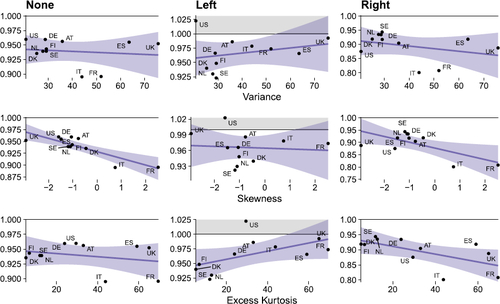
This discussion confirms that our model has the potential to improve upon simpler benchmarks by comparatively large margins. These improvements, however, are sometimes different across countries and one might ask what determines the differences. In particular, for h = 1, BART CC FM works particularly well for France and Italy in the right tail, while it is a bit worse for the US in the left tail. Hence, we analyze the cross-country relationship between unconditional features in the data and the one-step-ahead qw-CRPSs (ratios relative to the ABG benchmark).¹¹ The features we consider are the variance, skewness, and excess kurtosis.

Figure 2 shows these relationships in terms of cross-country scatterplots and regression relations. The latter have to be viewed with some caution given the small sample size involved. Nevertheless, two features stand out from the figure. First, about the left tail, the US seems a bit of an outlier, with the lowest variance of all countries. The four countries with the best left tail performance from BART CC FM (Sweden, Denmark, Finland, and Netherlands) are instead all characterized by very low excess kurtosis and tend to have low variance. Second, about the right tail, France is the country with the largest skewness and kurtosis, and Italy is also well above the average, in particular for skewness. We view this evidence of the roles of kurtosis and variance in driving tail forecast accuracy as a subject for future research.

Fig. 2 Relationship between predictive metrics for BART CC FM relative to the frequentist ABG (h = 1) and unconditional empirical moments of the underlying time series. Blue shaded areas refer to the 95% confidence interval.

A final interesting issue is whether the model ranking we have obtained is stable or not over time and, related, whether there are periods where the nonparametric models performed particularly well versus ABG, with the financial crisis and the Covid pandemic as episodes of particular interest. We shed light on this issue with Figure 3, which graphs the cumulative sum of indicated CRPS-variant for $h\in \{1,4\}$ relative to the ABG model, for QR CC and the overall best BART specifications.

Fig. 3 Relative cumulative sum of indicated CRPS-variant for $h\in \{1,4\}$ benchmarked to the frequentist ABG model, best overall BART specifications.

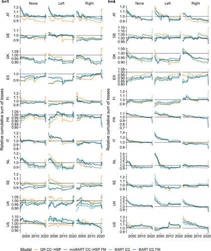
Overall, up until the pandemic, the time paths of relative performance accuracy are largely similar across the none, left, and right weighting schemes. Before the pandemic, for most countries, our proposed nonparametric forecasting approaches improve on the ABG benchmark in both the left and right tails.

The Covid period leads to some sizable shifts in relative performance that seem to drive some of the patterns in the full-sample results presented above. First, relative to ABG, our left tail results are helped by the Covid observations (i.e., score ratios are better in the full sample than in the sample ending in 2019). Second, in the right tail, the superiority of BART CC FM over BART CC seems to be driven by the Covid period. The better performance of our BART-based approaches relative to the standard QR can be attributed to the fact that the underlying forecast densities of the QR display a much larger predictive variance and in general more variation than the predictive distributions of the BART-based models (see the discussion in the next sub-section). Moreover, in the pre-Covid sample, BART CC is as good as (or sometimes slightly better than) BART CC FM. Furthermore, in several countries QR CC was rather good until the onset of the Covid period, so the excellent right tail performance of BART CC FM is at least in part driven by the pandemic. Specifically, in the case of the US the good right-tail performance also depends on the Covid period, typically not included in previous analysis on growth-at-risk, but the secular decline in CRPS ratios already started during/after the financial crisis. Finally, and related to the previous point, the financial crisis seems to have improved a bit the relative performance of the BART specifications, in particular for h = 1, though in general not to the point of changing the model rankings.

3.2.3 Properties of Growth Dynamics

Having shown that our set of nonparametric models yields excellent tail forecasts across countries, we now illustrate certain features of our model using estimates for the US, Italy, and Sweden.

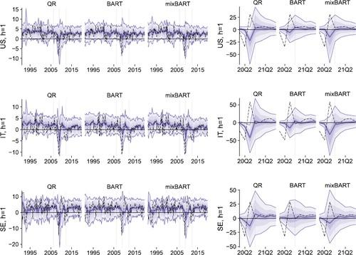
The first question that arises is whether the different models we propose yield predictive densities which are similar. This comparison is made in Figure 4, which shows the out-of-sample predictive distribution by quantile (posterior median) across QR, BART and mixBART, all for the CC FM model variant. Consider first the pre-pandemic sample that ends with 2019. One immediate observation is that, consistent with the literature, QR generates left-tail forecasts which are much more volatile than right-tail predictions, and particularly so during the great financial crisis. BART CC FM also yields more variability in left tail forecasts than right tail, but the left tail forecast is less variable for BART CC FM than QR. In left tail volatility, mixBART is somewhere between QR and BART. These patterns apply to all three countries. The pandemic portion of the sample produces larger changes in predictive distributions and much more variation across models. For all countries the QR forecasts are more variable over time than the BART forecasts, with mixBART’s forecasts generally somewhere in between. In addition, over this period the predictive densities are much wider with QR than BART, which turns out to contribute to BART’s relatively stronger forecast accuracy in the pandemic recovery. The stronger variation in the predictive density and the elevated predictive variance explain the weaker tail forecasting performance of linear QRs during the pandemic, highlighting that standard QRs have difficulties dealing with the outliers observed during the Covid period.

Fig. 4 Predictive distributions across CC FM model variants, HSP prior (when applicable). Blue shades cover the quantile pairs 5/95, 10/90, etc., alongside the median (blue line). Dashed lines mark realizations. Dotted vertical lines indicate selected quarters for which the full quantile function estimate is provided below.

To hone in on the statistical differences between our model specifications, we now consider several quarters (forecasts for 2006Q2, 2009Q1, 2012Q2, and 2020Q4) and plot the posterior quantiles of the estimated quantile function across specifications. These (also out-of-sample estimates) are shown in Figure 5. In rather quiet periods such as 2006Q2 and 2012Q2, we hardly find any differences in predictive quantiles. Instead, in the financial crisis (2009Q1), we find larger differences. These are particularly pronounced in the left tail, but are present also in other parts of the distribution, and for all the three countries.

Fig. 5 Posterior moments of the predictive quantile function for selected countries and quarters. We show the 68% credible set surrounding the median estimate. QR in gray, BART in blue, mixBART in red; CC FM and HSP prior (when applicable). Dashed lines mark realizations.

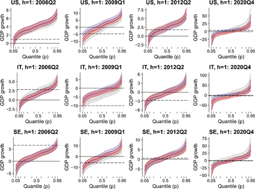
Finally, we consider 2020Q4. In that period, QR heavily over-predicts the right tail, but also the entire distribution seems shifted to the right for all three countries. This is driven by the fact that in the previous quarter, GDP growth strongly rebounded after the sharp decline during the first half of 2020. In the fourth quarter, however, GDP growth slowed, and the QR fails to capture this in the predictive distribution. This might be driven by the lack of flexibility when it comes to capturing rapid changes in the underlying time series. By contrast, both models that use BART appear to adjust quickly. In particular, the BART model produces predictive quantiles where both tails suggest more modest reactions of GDP growth, in line with the actual outcomes.

In the final part of this section we consider whether the different models give rise to different relations between the CISS and the conditional distribution of GDP growth, focusing on the US for the sake of space. Our framework allows us to analyze this question and back out how the conditional quantile functions vary with the CISS, keeping the other factors of the corresponding model at their unconditional means. This is achieved as follows. We vary the domestic CISS indicator (using a sequence of values between the minimum and maximum values over the full sample) and then assess how the implied quantile function changes. In this assessment, we use full-sample estimates of the models and the one-step-ahead forecast horizon.

Figure 6 shows the resulting estimates for the parametric linear, nonparametric, and combined function estimates for QR, BART, and mixBART. The first row shows $\mathit{\beta }{\prime }_{\mathit{\text{ip}}}{\mathit{x}}_{i,t}$ for mixBART and the QR, whereas the second row shows $g_{\mathit{\text{ip}}}({\mathit{x}}_{i,t})$ for BART and mixBART. Finally, the third row shows the sum over the linear and nonlinear part. The dashed lines are linear approximations to the estimated quantile function.

Fig. 6 Estimated functional relationship between the domestic CISS and GDP within each quantile in the United States. We show the 68% posterior credible set alongside the median. The dashed lines provide a linear approximation to the nonparametric functions. HSP prior when applicable.

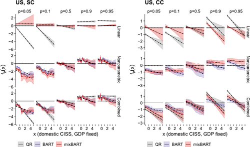
The left panels of the figure display the functional relations for single-country models. The findings indicate that the linear piece of mixBART is either constant and barely significant or centered on zero, implying no linear relationship between financial conditions and GDP growth. The QR essentially replicates the findings of ABG. In the left tail, the effect of financial conditions on growth is strong, whereas, in the middle of the distribution, the effect becomes weaker. In the upper tail, the QR implies the lack of a relationship.

When we consider the nonparametric piece and the combined mean relations, we find substantial evidence for nonlinearities in the left tail. For $p\in \{0.05,0.1\}$, the mean relationship (for both BART and mixBART models) suggests a rather linear but negative effect of the CISS on the left tail of GDP growth but if the CISS exceeds 1.5 the effect becomes much stronger. Afterwards, for larger values of the CISS the relationship becomes weaker until the regression relationship flattens out. This indicates that both models unveil a threshold effect in the left tail. The more we move into the center of the distribution, the more linear the effect becomes. Visually, this can be inspected by noting that the credible sets associated with the nonlinear function fully cover the linear approximation. The key difference to the standard QR is that we also detect negative but linear effects in the right tail of the conditional distribution.

Turning to the models that leverage cross-country information gives rise to a different picture. In that case, mixBART generates a linear effect that is negative in the left tail up to the median. For the right tail the effect remains sizable and negative. Interestingly, the results for the standard QR change markedly as well. Whereas we only find strong effects in the left tail for the single-country model (which is similar to the ABG benchmark), inclusion of cross-country information implies that the effects become much stronger for small values of the CISS and slightly weaker for larger values of the CISS. The key difference, however, is that we also observe strong negative relations in the right tail. By contrast, the nonparametric and combined effects become more linear and the kink at a CISS value of around 1.5 remains but is much less pronounced.

4 International Growth-at-Risk Dynamics

4.1 The Quantitative Importance of Nonparametric Features

In the previous section we have shown that our proposed framework yields forecast distributions which are often more accurate than the ones obtained from the ABG benchmark and simpler nested alternatives. One key advantage of the model is that it allows for varying importance of the nonparametric aspects across countries and quantiles and this improves forecasts in many cases. Moreover, at least for the US, nonlinearities seem to matter more in the tails than in the center of the distribution. We now assess whether this also holds for other countries and investigate in which parts of the distribution nonlinearities are relevant.

For this purpose, we compute the share of variance that is explained by BART relative to the combined linear and BART part in each conditional quantile for the mixBART specification: $\%{\text{BART}}_{\mathit{\text{ip}}}=\text{var}(g_{\mathit{\text{ip}}}({\mathit{X}}_i))/(\text{var}(g_{\mathit{\text{ip}}}({\mathit{X}}_i))+\text{var}({\mathit{X}}_i{\mathit{\beta }}_{\mathit{\text{ip}}}))$, where ${\mathit{X}}_i=({\mathit{x}}_{i,1},\dots ,{\mathit{x}}_{i,t})\prime$ is a T × K matrix. We compute these shares for each draw from the MCMC algorithm and then average them over time. The results over the full sample are depicted in Figure 7. To gauge the statistical significance, we indicate the 68% posterior credible set alongside the median.

Fig. 7 Decomposition of the explained variance for mixBART CC-HSP FM (end of sample), variance share explained by BART relative to the total explained variance. We show the 68% posterior credible set alongside the median.

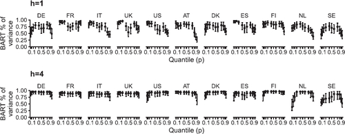
For h = 1, BART is relevant for all countries and percentiles, with values of the explained variance generally larger than 50%. These values are particularly pronounced in the left tail, approaching 100% for France, Italy, UK, US, Austria, Spain, and Finland. Yet, there are exceptions, in particular Germany, the Netherlands, and Sweden. For these countries, BART seems to matter more in the center of the predictive distribution. This heterogeneity provides further justification for our flexible approach. It is worth reiterating that BART can also approximate linear functions; this may yield a high share of variance for BART, even though the nonparametric function is approximately linear. For h = 4, the fraction of variance explained by BART further increases for virtually all countries and percentiles (with the exception of the left tail for the Netherlands), which is in line with the previous findings that nonlinearities become even more important at longer forecast horizons. In the Online Appendix we also provide information on how the posterior means of the shares change over the forecast evaluation sample. The values are quite stable over time, just a bit smaller at the beginning of the sample when the number of observations is lower.

As a rough gauge of variable importance, we compute selection frequencies of individual variables in the BART splitting rules. These results are again shown in the Online Appendix. Summarizing, for the domestic variants we find that the CISS covariate usually is selected more frequently than GDP growth. Differences between quantiles are negligible, as are differences between BART and mixBART. For our CC specifications, domestic economic conditions are chosen as splitting variables slightly more often on average. It is worth mentioning that all variables appear in the splitting rules.

4.2 The Role of the Common Factor

In this sub-section, we investigate the common factor across quantiles; for details about the implied covariance structure of our model, see the Online Appendix. In a first step, we assess the relevance of the common factor volatility specification by considering time averages of variance decompositions. These are obtained by leveraging the Gaussian representation of the AL (the distribution of ${ϵ}_{\mathit{\text{ip}},t}$ in (1)), as follows: $${\text{VD}}_{\mathit{\text{ip}},t}=\frac{{\lambda }_{\mathit{\text{ip}}}^2\hspace{0.17em}\mathrm{\text{exp}}\hspace{0.17em}(h_{p,t})}{{\lambda }_{\mathit{\text{ip}}}^2\hspace{0.17em}\mathrm{\text{exp}}\hspace{0.17em}(h_{p,t})+\text{var}({ϵ}_{\mathit{\text{ip}},t})},$$ with $\text{var}({ϵ}_{\mathit{\text{ip}},t})$ denoting the variance of ${ϵ}_{\mathit{\text{ip}},t}$. These shares are computed by drawing from the posteriors of the loadings, the log-volatilities and the augmentation parameters in (2). This yields a posterior distribution over variance shares and we report the posterior mean. This decomposition provides information on the share of variation in the shocks (conditional on the quantile) that is explained through the common factor (similar to Stock and Watson 2005).

Table 3 reports time averages of variance decompositions resulting from the BART CC FM model. Interestingly, for most countries the commonality is larger and more substantial in the tails than at the center of the distribution, and a bit larger in the right than in the left tail. These larger contributions in extreme periods can be traced back to the fact that several of the recessions in our hold-out period can be viewed as shocks with a pronounced global dimension (such as the global financial crisis or the Covid pandemic) and the factor is picking this up. Similarly, periods characterized by sharp expansions in business cycles have also been pretty synchronized across the countries we consider. The post-pandemic recovery, for instance, is a period where GDP growth rates increased markedly at roughly the same time across countries.

Table 3 Time averages of variance decompositions, BART CC FM.

Quantile (p)	AT	DE	DK	ES	FI	FR	IT	NL	SE	UK	US
0.05	0.85	0.84	0.79	0.83	0.77	0.86	0.84	0.84	0.86	0.87	0.82
0.10	0.77	0.72	0.63	0.77	0.61	0.80	0.76	0.73	0.76	0.77	0.75
0.25	0.63	0.59	0.42	0.61	0.38	0.56	0.61	0.56	0.53	0.61	0.58
0.50	0.83	0.68	0.30	0.95	0.21	0.98	0.90	0.56	0.40	0.89	0.71
0.75	0.79	0.76	0.50	0.77	0.48	0.80	0.81	0.69	0.59	0.78	0.69
0.90	0.83	0.85	0.68	0.81	0.65	0.85	0.84	0.79	0.75	0.82	0.77
0.95	0.91	0.91	0.82	0.90	0.82	0.92	0.91	0.89	0.87	0.92	0.87

Across countries, we find a considerable degree of homogeneity within country groups. For instance, Finland, Denmark, and Sweden feature commonalities that are very pronounced in the tails but decline once we approach the center of the distribution both from left and right. The US and the UK share a rather similar pattern in terms of commonalities (high shares in the tails and for the median, smaller shares for the quantiles in between).

The heterogeneity across quantiles in the role of the common factor is further supported by Figure 8, which reports estimates of the factors (upper panels) and associated log-volatility per quantile (lower panels). In the upper panel, we observe that especially in the tails the factor moves sharply during global events such as the global financial crisis and the Covid pandemic. To a somewhat smaller extent the results also suggest declines in the beginning of the 1990s and the early 2000s. When we focus attention on the 50% quantile we find strikingly different results. In the center of the distribution, the factor is small and very close to zero throughout the sample. During the pandemic we find a strong pronounced decrease in 2020Q2, which was triggered by an unprecedented downturn in real activity globally but also a strong increase in 2020Q3 (which was accompanied with sharply increasing GDP growth rates throughout all our countries).

Fig. 8 Estimates of factors and associated log-volatility per quantile, BART CC FM. We show the 68% and 90% posterior credible sets (shaded areas) alongside the median (solid line).

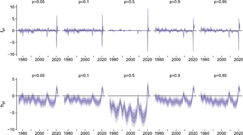
Turning to the evolution of the log-volatilities, the lower panel generally yields insights consistent with the findings discussed for the level of the factor. The log-volatility spikes during recessions (i.e., in the early 1990s, 2008/09, and 2020), and for p = 0.5 the level of the log-volatility is much smaller than for the other quantiles but then exceeds the increases in volatility observed for the other quantiles of the distribution. This finding also sheds light on why the amount of variation explained through the factor for most countries is lowest but still sizable in the 50% quantile. In most periods, the volatility of the common shock factor is small (around –5 to –10 on the log-scale) but then during the pandemic it rapidly increases and reaches values of around 5 on the log-scale. This suggests that in tranquil periods the factor only explains little variation in the shocks but in recessions (or turbulent times) this share increases appreciably and approaches 1.

To conclude, the Online Appendix considers how changes to the factor, labeled factor shocks, impact GDP growth across countries and quantiles (following Stock and Watson 2005). It turns out that a factor shock has different effects in the left tail than the right tail. In both tails, growth is negatively affected, but in QR estimates, the size of the effect (and persistence of the negative effect) is much larger in the left tail with respect to the nonparametric models. The Online Appendix also studies the international effects of a shock to US financial conditions, finding asymmetry in the sense that a positive shock affects the growth quantiles, whereas a negative shock’s effects are not as sharp. The responses are instead much more proportional and symmetric in the linear model, highlighting the importance of allowing for nonlinearities in the specification of quantile regressions.

5 Conclusions

In this article we propose a nonparametric quantile panel regression model which assumes that the quantiles depend on a set of predictors through nonlinear functions. We learn the unknown functions using BART. This nonparametric feature enhances model flexibility, especially in the tails. Using cross-sectional information, in addition, enables us to improve predictive accuracy. This is achieved by proposing a pooling prior as well as introducing cross-country information through latent heteroscedastic factors and lagged cross-country covariates. To carry out estimation and inference we design a scalable MCMC algorithm and apply the model to investigate growth-at-risk using a panel of 11 countries.

In terms of empirical results, our proposed models commonly improve on the benchmark ABG-style QR in recursive growth forecast comparisons, more so in the tails than near the center of the distribution. Moreover, some form of international information definitely pays off (modest improvements via a pooling prior, and more sizeable ones by outright including non-domestic series). The effects of the common factor are also relevant. In terms of predictions it often yields appreciable gains in forecast accuracy and, in-sample, it explains a large fraction of the forecast error variance in most countries, in particular in the tails.

The Covid period affects some of the patterns in the empirical results. In particular, relative to ABG, our left tail results are helped by the Covid observations; score ratios are better in the full sample than the in the sample ending in 2019. Moreover, in the pre-Covid sample, the factor is less relevant. Furthermore, in several countries QR with cross-sectional information was good also in the right tail until the onset of the Covid period, so the very good right tail performance of BART CC FM is at least partly driven by the Covid period.

Supplementary Materials

The online appendix includes additional details on the posterior simulation algorithm, robustness checks and additional empirical results.

Acknowledgments

The views expressed herein are solely those of the authors and do not necessarily reflect the views of the Federal Reserve Bank of Cleveland or the Federal Reserve System. We would like to thank the editor, the associate editor and a referee, as well as Ivan Petrella and Dimitris Korobilis for many helpful suggestions on earlier versions of the article.

Data Availability Statement

Codes and replication files are available at github.com/mpfarrho/qf-bart.

Disclosure Statement

The authors report there are no competing interests to declare.

Additional information

Funding

Marcellino thanks MIUR – PRIN Bando 2017 – prot. 2017TA7TYC for financial support; Huber and Pfarrhofer gratefully acknowledge financial support from the Austrian Science Fund (FWF, grant no. ZK 35).

Notes

1 Examples of exceptions include Korobilis et al. (2021) and Pfarrhofer (2022), which assume time variation in the quantile regression coefficients. However, even these papers are single-equation and assume particular parametric forms for the time variation. A multiple-equation exception is Adrian et al. (2022), which exploits information in the term structure for an empirical application involving linear panel quantile regression. Another one is the multivariate quantile regression developed in Iacopini, Ravazzolo, and Rossini (2022).

2 The density of AL ${}_p({\sigma }_p)$ is given by $p(1-p)/{\sigma }_p\hspace{0.17em}\mathrm{\text{exp}}\hspace{0.17em}(-{\rho }_p({ϵ}_t)/{\sigma }_p)$, where ${\rho }_p(x)=x(p-\mathbb{I}(x<0))$ is the check loss function and $\mathbb{I}(•)$ the usual indicator function. This does not imply that we assume the actual data to follow an AL distribution. For details on the correspondence between the Bayesian and classical approaches to inference in quantile regression, see Yu and Moyeed (2001).

3 Setting the full common mean to a zero vector of size K yields the conventional horseshoe (HS). The Online Appendix includes some comparisons of the HSP and HS priors. HSP typically has a small advantage over the HS version.

4 The density of the AL is provided in footnote 2, with $\mathbb{E}({ϵ}_{\mathit{\text{ip}},t})=[1-2p]/[p(1-p)]$ and Var $({ϵ}_{\mathit{\text{ip}},t})=[1-2p+2p^2]/[p^2{(1-p)}^2]$. Note that p determines the skewness of the distribution, and that its pth quantile is equal to zero. For our specific choices of θ_p and ${\tau }_p^2$, with independent standard normal variables $e_{\mathit{\text{ip}},t}\sim \mathcal{N}(0,1)$ and exponentially distributed $z_{\mathit{\text{ip}},t}\sim \mathcal{E}(1)$, it can be shown that the left- and right-hand side of (2) are equal in distribution; see chap. 3 in Kotz, Kozubowski, and Podgórski (2001) for a proof and additional details.

5 Note that all the techniques (including the MCMC algorithm in the Online Appendix) remain valid in this case. This is because in the Bayesian framework we implicitly condition on our model being true when we derive the full conditional posterior distributions.

6 For some empirical evidence on this claim, see Clark et al. (2023) who show that BART can produce accurate forecast distributions under homoscedastic shocks even if the DGP is heteroscedastic.

7 Additional details on how we compute the posterior densities of the quantile functions and other nonlinear functions of the parameters (such as impulse responses) are provided in the Online Appendix.

8 As opposed to directly modeling $400\times \hspace{0.17em}\mathrm{\text{log}}\hspace{0.17em}(Y_{i,T+h}/Y_{i,T})/h$, our approach has the advantage that we estimate a set of horizon-specific forecasting models and thus gain flexibility.

9 A shortcoming of this approach is that we treat the horizon-specific predictive densities as being independent. This assumption might be at odds with the data if the target series is persistent. To cope with this, Mogliani and Odendahl (2023) propose using copulas to capture horizon-specific correlations. In simulations, they show that the predictive gains from doing so are small if the data feature little persistence. Given that our target series is in growth rates we do not expect substantial improvements in predictive accuracy and hence treat the horizon-specific predictive densities as independent. This claim is also supported by our robustness checks in the Online Appendix.

10 Clark, Carriero, and Marcellino (2022) also find that ABG can be beaten in the right tail for the US.

11 The results for the four-steps-ahead qw-CRPSs are included in the Online Appendix.

References

- Adrian, T., Boyarchenko, N., and Giannone, D. (2019), “Vulnerable Growth,” American Economic Review, 109, 1263–89. DOI: 10.1257/aer.20161923.
- Adrian, T., Grinberg, F., Liang, N., Malik, S., and Yu, J. (2022), “The Term Structure of Growth-at-Risk,” American Economic Journal: Macroeconomics, 14, 283–323. DOI: 10.1257/mac.20180428.
- Bai, Y., Carriero, A., Clark, T. E., and Marcellino, M. (2022), “Macroeconomic Forecasting in a Multi-Country Context,” Journal of Applied Econometrics, 37, 1230–1255. DOI: 10.1002/jae.2923.
- Canova, F., and Ciccarelli, M. (2013), “Panel Vector Autoregressive Models: A Survey,” in VAR Models in Macroeconomics–New Developments and Applications: Essays in Honor of Christopher A. Sims (Vol. 32), pp. 205–246, Leeds: Emerald Publishing Ltd.
- Carriero, A., Clark, T. E., Marcellino, M., and Mertens, E. (in-press), “Addressing COVID-19 Outliers in BVARs with Stochastic Volatility,” Review of Economics and Statistics.
- Chipman, H. A., George, E. I., and McCulloch, R. E. (1998), “Bayesian CART Model Search,” Journal of the American Statistical Association, 93, 935–948. DOI: 10.1080/01621459.1998.10473750.
- Chipman, H. A., George, E. I., and McCulloch, R. E. (2010), “BART: Bayesian Additive Regression Trees,” The Annals of Applied Statistics, 4, 266–298.
- Clark, T., Carriero, A., and Marcellino, M. (2022), “Specification Choices in Quantile Regression for Empirical Macroeconomics,” Federal Reserve Bank of Cleveland working papers, 22–25.
- Clark, T. E., Huber, F., Koop, G., Marcellino, M., and Pfarrhofer. M. (2023), “Tail Forecasting with Multivariate Bayesian Additive Regression Trees,” International Economic Review, 64, 979–1022. DOI: 10.1111/iere.12619.
- Cook, T., and Doh, T. (2019), “Assessing Macroeconomic Tail Risks in a Data-Rich Environment,” Federal Reserve Bank of Kansas City Research working paper, 19–12.
- De Nicolò, G., and Lucchetta, M. (2017), “Forecasting Tail Risks,” Journal of Applied Econometrics, 32, 159–170. DOI: 10.1002/jae.2509.
- Delle Monache, D., De Polis, A., and Petrella, I. (2020), “Modeling and Forecasting Macroeconomic Downside Risk,” CEPR Discussion Paper Series, 15109.
- Diebold, F. X., and Mariano, R. S. (1995), “Comparing Predictive Accuracy,” Journal of Business & Economic Statistics, 13, 253–263. DOI: 10.2307/1392185.
- Feldkircher, M., Huber, F., Koop, G., and Pfarrhofer, M. (2022), “Approximate Bayesian Inference and Forecasting in Huge-Dimensional Multi-Country VARs,” International Economic Review, 63, 1625–1658. DOI: 10.1111/iere.12577.
- Ferrara, L., Mogliani, M., and Sahuc, J. G. (2022), “High-Frequency Monitoring of Growth at Risk,” International Journal of Forecasting, 38, 582–595. DOI: 10.1016/j.ijforecast.2021.06.010.
- Figueres, J. M., and Jarociński, M. (2020), “Vulnerable Growth in the Euro Area: Measuring the Financial Conditions,” Economics Letters, 191, 109126. DOI: 10.1016/j.econlet.2020.109126.
- Gaglianone, W. P., and Lima, L. R. (2012), “Constructing Density Forecasts from Quantile Regressions,” Journal of Money, Credit and Banking, 44, 1589–1607. DOI: 10.1111/j.1538-4616.2012.00545.x.
- Galbraith, J. W., and van Norden, S. (2019), “Asymmetry in Unemployment Rate Forecast Errors,” International Journal of Forecasting, 35, 1613–1626. DOI: 10.1016/j.ijforecast.2018.11.006.
- Ghysels, E., Iania, L., and Striaukas, J. (2018), “Quantile-based Inflation Risk Models,” National Bank of Belgium Research Working Paper, 349.
- Giglio, S., Kelly, B., and Pruitt, S. (2016), “Systemic Risk and the Macroeconomy: An Empirical Evaluation,” Journal of Financial Economics, 119, 457–471. DOI: 10.1016/j.jfineco.2016.01.010.
- Gneiting, T., and Ranjan, R. (2011), “Comparing Density Forecasts Using Threshold- and Quantile-Weighted Scoring Rules,” Journal of Business & Economic Statistics, 29, 411–422. DOI: 10.1198/jbes.2010.08110.
- González-Rivera, G., Maldonado, J., and Ruiz, E. (2019), “Growth in Stress,” International Journal of Forecasting, 35, 948–966. DOI: 10.1016/j.ijforecast.2019.04.006.
- Huber, F., Koop, G., Onorante, L., Pfarrhofer, M., and Schreiner, J. (2023), “Nowcasting in a Pandemic Using Non-parametric Mixed Frequency VARs,” Journal of Econometrics, 232, 52–69. DOI: 10.1016/j.jeconom.2020.11.006.
- Huber, F., and Rossini, L. (2022), “Inference in Bayesian Additive Vector Autoregressive Tree models,” The Annals of Applied Statistics, 16, 104–123. DOI: 10.1214/21-AOAS1488.
- Iacopini, M., Ravazzolo, F., and Rossini, L. (2022), “Bayesian Multivariate Quantile Regression with Alternative Time-Varying Volatility Specifications,” arXiv, 2211.16121.
- Kiley, M. T. (2022), “Unemployment Risk,” Journal of Money, Credit and Banking, 54, 1407–1424. DOI: 10.1111/jmcb.12888.
- Korobilis, D. (2017), “Quantile Regression Forecasts of Inflation under Model Uncertainty,” International Journal of Forecasting, 33, 11–20. DOI: 10.1016/j.ijforecast.2016.07.005.
- Korobilis, D., Landau, B., Musso, A., and Phella, A. (2021), “The Time-Varying Evolution of Inflation Risks,” ECB working paper series, 2600.
- Kose, M. A., Otrok, C., and Whiteman, C. H. (2003), “International Business Cycles: World, Region, and Country-Specific Factors,” American Economic Review, 93, 1216–1239. DOI: 10.1257/000282803769206278.
- Kotz, S., Kozubowski, T., and Podgórski, K. (2001), The Laplace Distribution and Generalizations: A Revisit with Applications to Communications, Economics, Engineering, and Finance (Vol. 183), Boston, MA: Springer.
- Kozumi, H., and Kobayashi, G. (2011), “Gibbs Sampling Methods for Bayesian Quantile Regression,” Journal of Statistical Computation and Simulation, 81, 1565–1578. DOI: 10.1080/00949655.2010.496117.
- Lusompa, A. (2023), “Local Projections, Autocorrelation, and Efficiency,” Quantitative Economics, 14, 1199–1220. DOI: 10.3982/QE1988.
- Manzan S. (2015), “Forecasting the Distribution of Economic Variables in a Data-Rich Environment,” Journal of Business and Economic Statistics, 33, 144–164. DOI: 10.1080/07350015.2014.937436.
- Manzan, S., and Zerom, D. (2013), “Are Macroeconomic Variables Useful for Forecasting the Distribution of US Inflation?” International Journal of Forecasting, 29, 469–478. DOI: 10.1016/j.ijforecast.2013.01.005.
- Marcellino, M., Stock, J. H., and Watson, M. W. (2006), “A Comparison of Direct and Iterated Multistep AR Methods for Forecasting Macroeconomic Time Series,” Journal of Econometrics, 135, 499–526. DOI: 10.1016/j.jeconom.2005.07.020.
- Mitchell, J., Poon, A., and Mazzi, G. L. (2022), “Nowcasting Euro Area GDP Growth Using Quantile Regression,” Advances in Econometrics, 43A, 51–72.
- Mitchell, J., Poon, A., and Zhu, D. (2023), “Constructing Density Forecasts from Quantile Regressions: Multimodality in Macro-Financial Dynamics,” FRB of Cleveland working pper, 22-12R.
- Mogliani, M., and Odendahl, F. (2023), “Density Forecast Frequency Transformation via Copulas,” mimeo.
- Pfarrhofer, M. (2022), “Modeling Tail Risks of Inflation Using Unobserved Component Quantile Regressions,” Journal of Economic Dynamics and Control, 143, 104493. DOI: 10.1016/j.jedc.2022.104493.
- Plagborg-Møller, M., Reichlin, L., Ricco, G., and Hasenzagl, T. (2020), “When is Growth at Risk?” Brookings Papers on Economic Activity, pp. 167–229. DOI: 10.1353/eca.2020.0002.
- Reichlin, L., Ricco, G., and Hasenzagl, T. (2020), “Financial Variables as Predictors of Real Growth Vulnerability,” Deutsche Bundesbank Discussion paper, 05/2020.
- Stock, J. H., and Watson, M. W. (2005), “Understanding Changes in International Business Cycle Dynamics,” Journal of the European Economic Association, 3, 968–1006. DOI: 10.1162/1542476054729446.
- Taddy, M., and Kottas, A. (2010), “A Bayesian Nonparametric Approach to Inference for Quantile Regression,” Journal of Business and Economic Statistics, 28, 357–369. DOI: 10.1198/jbes.2009.07331.
- Yu, K., and Moyeed, R. A. (2001), “Bayesian Quantile Regression,” Statistics & Probability Letters, 54, 437–447. DOI: 10.1016/S0167-7152(01)00124-9.