Max Share Identification of Multiple Shocks: An Application to Uncertainty and Financial Conditions

Abstract

We generalize the Max Share approach to allow for simultaneous identification of a multiplicity of shocks in a Structural Vector Autoregression. Our machinery therefore overcomes the well-known drawbacks that individually identified shocks (i) tend to be correlated to each other or (ii) can be separated under orthogonalizations with weak economic ground. We show that identification corresponds to solving a nontrivial optimization problem. We provide conditions for non-emptiness of solutions and point-identification, and Bayesian algorithms for estimation and inference. We use the approach to study the effects of uncertainty and financial shocks, allowing for the possibility that the former responds contemporaneously to other shocks, distinguishing macroeconomic from financial uncertainty and credit supply shocks. Using U.S. data we find that financial uncertainty mimics a demand shock, while the interpretation of macro uncertainty is more mixed. Furthermore, variation in uncertainty partially represents the endogenous response of uncertainty to other shocks.

KEYWORDS:

• Causality
• Forecast error variance
• Identification
• Structural vector autoregression
• Uncertainty

1 Introduction and Related Literature

Since the contribution of Sims (1980), structural vector autoregressions (SVARs) are the typical toolkit for investigating the dynamic effects caused by macroeconomic shocks. While early studies employed zero short-run, sign and long-run restrictions on impulse response functions (IRFs) for the identification of structural shocks (Sims 1980; Blanchard and Quah 1989; Uhlig 2005), a most recent device, known as Max Share identification, constrains the Forecast Error Variance Decomposition (FEVD) of target variables (Uhlig 2004). For example, this approach identifies technology shocks as those which explain the most of the FEVD of labor productivity at 10-year period (Francis et al.2014). Other applications include DiCecio and Owyang (2010) (technology shocks), Barsky and Sims (2011) and Kurmann and Sims (2021) (news shocks), Mumtaz, Pinter, and Theodoridis (2018) (credit shocks), Mumtaz and Theodoridis (2023) (inflation target shocks), Caldara et al. (2016) (uncertainty and credit shocks), Levchenko and Pandalai-Nayar (2020) (sentiment shocks) and Angeletos, Collard, and Dellas (2020) (a variety of supply and demand shocks).

The Max Share approach is common because its implementation is easy and delivers less biased impulse responses than standard long run restrictions (Francis et al.2014). However, it presents two drawbacks. First, it can identify only one shock at a time. This makes the identified shock be often correlated with other disturbances; as such it is not truly structural. For instance, Cascaldi-Garcia and Galvão (2021) find that uncertainty and news shocks, if singularly identified, are strongly correlated. Thus, literature has been adopting a sequential procedure, where Max Share is applied to orthogonalized shocks. In practice, orthogonalizations rely on arbitrary ordering restrictions, making any economic interpretation hard (Uhlig 2004). For example, Caldara et al. (2016) apply the Max Share identification to sequentially identify uncertainty and financial shocks, finding that changing the order of identification dramatically affects the results, for example uncertainty can be both expansionary and recessionary. Second, Max Share confounds shocks (Giannone, Lenza, and Reichlin 2019; Dieppe, Francis, and Kindberg-Hanlon 2021; Kurmann and Sims 2021); identified disturbances tend to be a linear combination of the truly structural shocks.

In this article, we generalize the Max Share toolkit to identification of a multiplicity of shocks. Instead of constraining the FEV to a single shock, we simultaneously restrict (a function of) the FEV of target variables to more shocks. Researchers have been increasingly identifying more shocks (Mertens and Ravn 2013; Furlanetto, Ravazzolo, and Sarferaz 2017; Piffer and Podstawski 2018; Brianti 2021; Cascaldi-Garcia and Galvão 2021; Ludvigson, Ma, and Ng 2021; Giacomini, Kitagawa, and Read 2022); while some strategies, such as sign restrictions and proxy SVARs, allow for identification of a multiplicity of disturbances, the methodological contribution of this article is to make the Max Share identification suitable for more shocks. This addresses the problem of sequential identification implied by the standard Max Share approach and mitigates the issue of shocks confounding.

Our identification strategy involves the solution of a constrained maximization problem, where the objective function is an equally weighted linear combination of the FEVD of the (target) variables of interest and the constraints are the inequality restrictions on the FEVD, that is on the contributions of the shocks to the FEV of different variables (for instance, in our application, macro uncertainty shocks explain variation of macro uncertainty proxy more than the fluctuation in credit spreads). Depending on the application, those restrictions can be replaced by, or combined with, traditional sign restrictions. We show that the problem corresponds to a non-convex quadratic optimization on the columns of the rotation matrix transforming reduced-form residuals into structural shocks. However, we provide a flexible toolkit and establish mild conditions under which the solution of the optimization problem exists (non-emptiness of the identified set) and is unique (point-identification). We develop simple algorithms to perform Bayesian estimation and inference, even though of course the identification result and properties do hold also in a frequentist setting.

A simulation exercise shows that our approach recovers the impulse response functions in different Data Generating Processes (DGPs) and mitigates the problem of confounded shocks.

Turning to the empirical application, we apply the proposed identification scheme to a SVAR model estimated with U.S. data and identify macro uncertainty, financial uncertainty and pure financial (credit supply) shocks. Since the influential paper of Bloom (2009), the business cycle relationship between uncertainty and macroeconomic variables has received extensive consideration (Bloom (2014) provides an excellent survey). Three challenges come to the fore. First, the common assumption in empirical works is that uncertainty is exogenous, that is it does not respond contemporaneously to economic variables. However, the current evidence makes researchers unable to take up a position on the direction of the causality between uncertainty and economic variables. Henceforth, we use the terms exogenous (endogenous) as shorthand for predetermined (not predetermined) within the period.

A separate challenge is about the origins of uncertainty. Standard theories claim that uncertainty originates from macroeconomic fundamentals, for example productivity. However, it has been argued that uncertainty can depress the economy through sources of uncertainty specific to financial markets (Bollerslev, Tauchen, and Zhou 2009; Ng and Wright 2013). The current literature does not disentangle the contributions of macroeconomic versus financial uncertainty to business cycle fluctuations, nor does it allows feedback between macroeconomic and financial uncertainty. Exceptions are the small-scale models in Ludvigson, Ma, and Ng (2021) and Angelini et al. (2019) and the contribution in Shin and Zhong (2020).

While Furlanetto, Ravazzolo, and Sarferaz (2017), Caldara et al. (2016), Caggiano et al. (2021), and Brianti (2021) extensively discuss the need to identify credit shocks to sharpen identification of uncertainty shocks accordingly, there is high degree of comovement between indicators of financial distress and uncertainty proxies (Caldara et al.2016; Brianti 2021; Caggiano et al.2021); also, uncertainty and financial shocks have theoretically the same qualitative effects on both prices and quantities. It is therefore difficult to impose plausible zero or sign restrictions to identify these two disturbances.

Our approach deals with the three issues above. We find that financial uncertainty shocks act as negative demand shocks, that is decrease real activity; increase in macro uncertainty leads to a recession, but the effect on prices is much more mixed. The responses to the two shocks are also quantitatively different: macroeconomic uncertainty has a stronger and more persistent effect on the real activity variables. Our results show that uncertainty is endogenous to some extent, in the sense that a nontrivial share of the variance of measures of uncertainty represents endogenous responses to non-uncertainty shocks. Finally, increases in credit spreads trigger a recession.

The article is organized as follows. Section 2 provides the econometrics framework and the standard Max Share identification; Section 3 introduces our approach and its properties; Section 4 presents the empirical application; Section 5 concludes. A separate supplemental Appendix provides full proofs (Appendix A), validation of the identification approach through fully structural models (Appendix B), additional details about the simulation exercises (Appendix C), robustness checks (Appendix D), detailed description of the algorithms (Appendix E), generalization to the frequency domain (Appendix F) and further extensions (Appendix G and H).

2 Theoretical Framework

Consider a SVAR(p) model (2.1) $${\mathit{A}}_0{\mathit{y}}_t=\mathit{a}+\sum _{j=1}^p{\mathit{A}}_j{\mathit{y}}_{t-j}+{\mathit{ϵ}}_t$$(2.1) for $t=1,\dots ,T,$ where ${\mathit{y}}_t$ is an $n\times 1$ vector of endogenous variables, ${\mathit{ϵ}}_t$ an $n\times 1$ vector white noise process, normally distributed with mean zero and variance-covariance matrix ${\mathit{I}}_n$, ${\mathit{A}}_j$ is an n × n matrix of structural coefficient for $j=0,\dots ,p$. The disturbances ${\mathit{ϵ}}_t$ are mutually uncorrelated, and are therefore interpretable as structural shocks. The initial conditions ${\mathit{y}}_1,\dots ,{\mathit{y}}_p$ are given. Let $\mathit{\theta }=({\mathit{A}}_0,{\mathit{A}}_{+})$ collect the structural parameters, where ${\mathit{A}}_{+}=(\mathit{a},{\mathit{A}}_j)$ for $j=1,\dots ,p$.

The reduced-form representation is a Vector Autoregression (VAR): (2.2) $${\mathit{y}}_t=\mathit{b}+\sum _{j=1}^p{\mathit{B}}_j{\mathit{y}}_{t-j}+{\mathit{u}}_t,$$(2.2) where $\mathit{b}={\mathit{A}}_0^{-1}\mathit{a}$ is an $n\times 1$ vector of constants, ${\mathit{B}}_j={\mathit{A}}_0^{-1}{\mathit{A}}_j$, ${\mathit{u}}_t={\mathit{A}}_0^{-1}{\mathit{ϵ}}_t$ denotes the $n\times 1$ vector of reduced-form errors. $\mathit{\text{var}}({\mathit{u}}_t)=E({\mathit{u}}_t\mathit{u}{\prime }_t)=\mathbf{\Sigma }={\mathit{A}}_0^{-1}({\mathit{A}}_0^{-1})\prime$ is the n × n variance-covariance matrix of reduced-form errors. Let $\mathit{\varphi }=(\mathit{B},\mathbf{\Sigma })\in \mathbf{\Phi }$ collect the reduced-form parameters, where $\mathit{B}\equiv \left[\mathit{b},{\mathit{B}}_1,\dots ,{\mathit{B}}_p\right],\mathbf{\Phi }\subset {\mathcal{R}}^{n+n^{2}p}\times \mathbf{\Xi }$, and $\mathbf{\Xi }$ is the space of symmetric positive semidefinite matrices.

We define the n × n matrix (2.3) $$\mathit{I}{\mathit{R}}^h={\mathit{C}}_h(\mathit{B}){\mathit{A}}_0^{-1}$$(2.3) as the impulse response at hth horizon for $h=0,1,\dots$, where ${\mathit{C}}_h(\mathit{B})$ is the hth coefficient matrix of ${({\mathit{I}}_n-{\sum }_{h=1}^p{\mathit{B}}_h{L}^h)}^{-1}$. Its (i, j)-element denotes the effect on the ith variable in ${\mathit{y}}_{t+h}$ of a unit shock to the jth element of ${\mathit{ϵ}}_t$. As is well-known there are several observationally equivalent ${\mathit{A}}_0$ matrices, and expression (2.3) actually involves a set of impulse responses.

To formalize this fact we follow Uhlig (2005) and define the set of all IRFs through an n × n orthonormal matrix $\mathit{Q}\in \mathbf{\Theta }(n)$, where $\mathbf{\Theta }(n)$ characterizes the set of all orthonormal n × n matrices. Uhlig (2005) show that $\{{\mathit{A}}_0=\mathit{Q}\prime {\mathbf{\Sigma }}_{\mathit{\text{tr}}}^{-1}:\mathit{Q}\in \mathbf{\Theta }(n)\}$ is the set of observationally equivalent ${\mathit{A}}_0$’s consistent with reduced-form parameters, where $\mathbf{\Sigma }$ relates to ${\mathit{A}}_0$ by $\mathbf{\Sigma }={\mathit{A}}_0^{-1}{({\mathit{A}}_0^{-1})}^{\prime }$, ${\mathbf{\Sigma }}_{\mathit{\text{tr}}}$ denotes the lower triangular Cholesky matrix with nonnegative diagonal coefficients of $\mathbf{\Sigma }$. The likelihood function depends on $\mathit{\varphi }$ and does not contain any information about Q, leading to ambiguity in decomposing $\mathbf{\Sigma }$. The identification problem arises because there is a multiplicity of Q’s which deliver ${\mathit{A}}_0$ given $\mathit{\varphi }$. Specifically, the impulse response of variable i to shock j at horizon h, that is (i, j)-element of $\mathit{I}{\mathit{R}}^h$, can be expressed as $\mathit{e}{\prime }_i{\mathit{C}}_h(\mathit{B}){\mathbf{\Sigma }}_{\mathit{\text{tr}}}\mathit{Q}{\mathit{e}}_j\equiv \mathit{c}{\prime }_{\mathit{\text{ih}}}(\mathit{\varphi }){\mathit{q}}_j$, where ${\mathit{e}}_i$ is the ith column vector of ${\mathit{I}}_n,{\mathit{q}}_j$ is the jth column of Q and $\mathit{c}{\prime }_{\mathit{\text{ih}}}(\mathit{\varphi })$ represents the ith row vector of ${\mathit{C}}_h(\mathit{B}){\mathbf{\Sigma }}_{\mathit{\text{tr}}}$. Alternative identification schemes can be achieved by placing a set of restrictions on Q. For example, imposing $\mathit{Q}={\mathit{I}}_n$ implies a recursive ordering identification, that is the Cholesky decomposition, whereas sign restrictions specify a set of admissible Q’s.

2.1 Sign Restrictions

Before introducing our identification toolkit, we review the sign restrictions, which are often combined with the Max Share identification in empirical applications. Assume that the researcher is interested in imposing some sign restrictions on the impulse response vector to the jth structural shock, and let s_hj denote the number of sign restrictions on impulse responses at horizon h. In this case, the impulse response is given by the jth column vector of $\mathit{I}{\mathit{R}}^h={\mathit{C}}_h(\mathit{B}){\mathbf{\Sigma }}_{\mathit{\text{tr}}}\mathit{Q}$, and the sign restrictions are $${\mathit{S}}_{\mathit{\text{hj}}}(\mathit{\varphi }){\mathit{q}}_j\ge \mathbf{0},$$where ${\mathit{S}}_{\mathit{\text{hj}}}(\mathit{\varphi })\equiv {\mathit{D}}_{\mathit{\text{hj}}}{\mathit{C}}_h(\mathit{B}){\mathbf{\Sigma }}_{\mathit{\text{tr}}}$ is a $s_{\mathit{\text{hj}}}\times n$ matrix and ${\mathit{D}}_{\mathit{\text{hj}}}$ is the $s_{\mathit{\text{hj}}}\times n$ selection matrix that selects the sign-restricted responses from the $n\times 1$ response vector ${\mathit{C}}_h(\mathit{B}){\mathbf{\Sigma }}_{\mathit{\text{tr}}}{\mathit{q}}_j$. The nonzero elements of ${\mathit{D}}_{\mathit{\text{hj}}}$ can be equal to 1 or to–1 depending on the sign of the restriction on the impulse response of interest. By considering multiple horizons, the whole set of sign restrictions placed on the jth shock is (2.4) $${\mathit{S}}_j(\mathit{\varphi }){\mathit{q}}_j\ge \mathbf{0}.$$(2.4)

Specifically, ${\mathit{S}}_j$ is a $({\sum }_{h=0}^{{\overline{h}}_j}{s}_{\mathit{\text{hj}}})\times n$ matrix defined by ${\mathit{S}}_j(\mathit{\varphi })=\left[\mathit{S}{\prime }_{0j}(\mathit{\varphi }),\dots ,\mathit{S}{\prime }_{{\overline{h}}_{j}j}(\mathit{\varphi })\right]\prime$. Let ${\mathcal{I}}_{\mathcal{S}}\subset \{1,2,\dots ,n\}$ be the set of indices such that $j\in {\mathcal{I}}_{\mathcal{S}}$ if some of the impulse responses to the jth structural shock are sign-constrained. Thus, the set of all sign restrictions is (2.5) $${\mathit{S}}_j(\mathit{\varphi }){\mathit{q}}_j\ge \mathbf{0},\text{for}j\in {\mathcal{I}}_{\mathcal{S}}.$$(2.5)

2.2 The Forecast Error Variance

Given the available information up to t–1, $\mathit{\text{FE}}(h)\equiv {\mathit{y}}_{t+\tilde{h}}-{\mathit{y}}_{t+\tilde{h}|t-1}$ is the $\tilde{h}$-step ahead forecast error. The Forecast Error Variance at $\tilde{h}$ is

$\mathit{\text{FEV}}(\tilde{h})\equiv E\left[({\mathit{y}}_{t+\tilde{h}}-{\mathit{y}}_{t+\tilde{h}|t-1})({\mathit{y}}_{t+\tilde{h}}-{\mathit{y}}_{t+\tilde{h}|t-1})\prime \right]={\sum }_{h=0}^{\tilde{h}}\mathit{I}{\mathit{R}}^h\mathit{I}{\mathit{R}}^{h\prime }$. Thus, ${\mathit{\text{CFEV}}}_j^i(\tilde{h})$ denotes the FEV at horizon $\tilde{h}$ of variable i explained by the jth structural shock—expressed with a number in the interval $[0,1]$ -: (2.6) $${\mathit{\text{CFEV}}}_j^i(\tilde{h})=\mathit{q}{\prime }_j{\mathbf{\Upsilon }}_{\tilde{\mathit{h}}}^{\mathit{i}}(\mathit{\varphi }){\mathit{q}}_j,$$(2.6) where ${\mathbf{\Upsilon }}_{\tilde{\mathit{h}}}^{\mathit{i}}(\mathit{\varphi })=\frac{{\sum }_{h=0}^{\tilde{h}}{\mathit{c}}_{\mathit{\text{ih}}}(\mathit{\varphi })\mathit{c}{\prime }_{\mathit{\text{ih}}}(\mathit{\varphi })}{{\sum }_{h=0}^{\tilde{h}}\mathit{c}{\prime }_{\mathit{\text{ih}}}(\mathit{\varphi }){\mathit{c}}_{\mathit{\text{ih}}}(\mathit{\varphi })}$ is a n × n positive semidefinite matrix. This is typically employed to illustrate the sources of variables’ fluctuation at different horizons.

2.3 Standard Max Share Identification

Uhlig (2004) and subsequent literature propose to identify shocks by maximizing the FEV of a target variable i to the shock of interest j: (2.7) $${\mathit{q}}_{j^{*}}=\underset{{\mathit{q}}_j}{\mathrm{\text{arg}}\max }\mathit{q}{\prime }_j{\mathbf{\Upsilon }}_{\tilde{\mathit{h}}}^{\mathit{i}}(\mathit{\varphi }){\mathit{q}}_j$$(2.7) subject to (2.8) $${\mathit{S}}_j(\mathit{\varphi }){\mathit{q}}_j\ge \mathbf{0},\text{for}j\in {\mathcal{I}}_{\mathcal{S}}$$(2.8) and (2.9) $$\mathit{q}{\prime }_j{\mathit{q}}_j=1.$$(2.9)

This is a convex and user-friendly problem; for example, in absence of sign restrictions, ${\mathit{q}}_{j^{*}}$ is the eigenvector corresponding to the highest eigenvalue of the reduced-form matrix ${\mathbf{\Upsilon }}_{\tilde{\mathit{h}}}^{\mathit{i}}(\mathit{\varphi })$. For instance, Francis et al. (2014) identify a technology shock as the shock with the maximum contribution to the FEV of labor productivity at the 10-year horizon (e.g., $\tilde{h}=40$ with quarterly data).

However, this approach presents two drawbacks. First, in presence of more than one shock of interest, Max Share identification is sequentially applied on orthogonalized shocks. In practice, orthogonalizations rely on arbitrary ordering restrictions. For example, in an n-variable system if there are two shocks of interest, the first shock might be identified as the shock that has the maximum contribution to the FEV of variable 1 over some horizon. This point-identifies ${\mathit{q}}_1$. The second shock might then be identified as the shock that has the maximum contribution to the FEV of variable 2 over some horizon, subject to the constraint ${\mathit{q}}_2^{\prime }{\mathit{q}}_1=0$ (i.e., so the two identified shocks are uncorrelated). Second, Max Share identification tends to confound shocks, that is delivers identified shocks that are a linear combination of the truly structural disturbances. The following bivariate example analytically illustrates the methodology and its issues.

Example 2.1.

Appendix A.2 provides the proof of the results in this example. The structural framework of the bivariate SVAR(0) is the following (adding some dynamics would not change the spirit of the findings): (2.10) $${\mathit{A}}_0\left(\begin{array}{c}{y}_{1t}\\ y_{2t}\end{array}\right)=\left(\begin{array}{c}{ϵ}_{1t}\\ {ϵ}_{2t}\end{array}\right),{\mathit{A}}_0=\left(\begin{array}{cc}{a}_{11}& a_{12}\\ a_{21}& a_{22}\end{array}\right),t=1,\dots ,T,$$(2.10) where $(y_{1t},y_{2t})$ are two endogenous variables, respectively. $({ϵ}_{1t},{ϵ}_{2t})$ denotes an iid normally distributed vector of structural shocks with variance-covariance the identity matrix. $\mathit{\theta }={\mathit{A}}_0$ collects the structural parameters, and the contemporaneous impulse responses are elements of ${\mathit{A}}_0^{-1}$. The reduced-form model is indexed by $\mathbf{\Sigma }$ (the variance-covariance matrix of the endogenous variables), which satisfies $\mathbf{\Sigma }={\mathit{A}}_0^{-1}{({\mathit{A}}_0^{-1})}^{\prime }$. Let ${\mathbf{\Sigma }}_{\mathit{\text{tr}}}=(\begin{array}{cc}{\sigma }_{11}& 0\\ {\sigma }_{21}& {\sigma }_{22}\end{array})$ denote its lower triangular Cholesky decomposition, where ${\sigma }_{11}>0,{\sigma }_{22}>0$, and ${\sigma }_{21}<0$ (the latter for simplicity, without loss of generalization). Thus, $\mathit{\varphi }=({\sigma }_{11},{\sigma }_{21},{\sigma }_{22})$ collects the reduced-form parameters. Following the example of Uhlig (2005), ${\mathit{A}}_0$ can be parameterized via the Cholesky matrix ${\mathbf{\Sigma }}_{\mathit{\text{tr}}}$ and a rotation matrix $\mathit{Q}=(\begin{array}{cc}\hspace{0.17em}\mathrm{\text{cos}}\hspace{0.17em}\rho & -\hspace{0.17em}\mathrm{\text{sin}}\hspace{0.17em}\rho \\ \hspace{0.17em}\mathrm{\text{sin}}\hspace{0.17em}\rho & \hspace{0.17em}\mathrm{\text{cos}}\hspace{0.17em}\rho \end{array})$ with spherical coordinate $\rho \in [0,2\pi ]$. The structural matrix of impact responses can be written as (2.11) $$\begin{array}{c}\mathit{I}{\mathit{R}}^0={\mathit{A}}_0^{-1}={\mathbf{\Sigma }}_{\mathit{\text{tr}}}\mathit{Q}\\ =\left(\begin{array}{cc}{\sigma }_{11}\hspace{0.17em}\mathrm{\text{cos}}\hspace{0.17em}\rho & -{\sigma }_{11}\hspace{0.17em}\mathrm{\text{sin}}\hspace{0.17em}\rho \\ {\sigma }_{21}\hspace{0.17em}\mathrm{\text{cos}}\hspace{0.17em}\rho +{\sigma }_{22}\hspace{0.17em}\mathrm{\text{sin}}\hspace{0.17em}\rho & -{\sigma }_{21}\hspace{0.17em}\mathrm{\text{sin}}\hspace{0.17em}\rho +{\sigma }_{22}\hspace{0.17em}\mathrm{\text{cos}}\hspace{0.17em}\rho \end{array}\right).\end{array}$$(2.11)

For simplicity, we assume no sign constraints other than the normalizations: ${\sigma }_{11}\hspace{0.17em}\mathrm{\text{cos}}\hspace{0.17em}\rho \ge 0$ and $-{\sigma }_{21}\hspace{0.17em}\mathrm{\text{sin}}\hspace{0.17em}\rho +{\sigma }_{22}\hspace{0.17em}\mathrm{\text{cos}}\hspace{0.17em}\rho \ge 0$. Let ${\mathit{Q}}_{\mathit{\text{ij}}}$ and $\mathit{I}{\mathit{R}}_{\mathit{\text{ij}}}^0$ denote the ijth element of the two matrices.

We are interested in identifying ${\mathit{q}}_1$ and ${\mathit{q}}_2$. Suppose that we apply the Max Share identification to ${\mathit{q}}_1$ first, that is the first shock is identified as the shock that has the maximum contribution to the one-step-ahead FEV of the first variable. As a result, ${\mathit{q}}_2$ is derived as the orthogonalized vector to ${\mathit{q}}_1$. In this case, the Appendix shows that ${ϵ}_{1t}=\hspace{0.17em}\mathrm{\text{cos}}\hspace{0.17em}\rho {ϵ}_{1t\mathit{\text{DGP}}}-\hspace{0.17em}\mathrm{\text{sin}}\hspace{0.17em}\rho {ϵ}_{2t\mathit{\text{DGP}}}$, where ${ϵ}_{1t\mathit{\text{DGP}}}$ and ${ϵ}_{2t\mathit{\text{DGP}}}$ are the shocks in the DGP. Unless the DGP satisfies the restriction ρ = 1 (equivalently, $\mathit{I}{\mathit{R}}_{11}^0={\sigma }_{11}$, that is the first shock explains 100 per cent of the one-step-ahead forecast error variance of the first variable), the identified shock is a linear combination of the true shocks. A similar argument applies when ${ϵ}_{2t}$ is identified via the standard Max Share, where the second shock explains 100 per cent of the one-step-ahead forecast error variance of the second variable (see the Appendix).

This illustrates that (i) order of orthogonalization changes the impulse responses and (ii) Max Share confounds shocks. Given the bivariate setting, identifying one column of Q mechanically pins down the other one. However, (i) and (ii) are general to the n-variable case, for example Dieppe, Francis, and Kindberg-Hanlon (2021).

3 Generalizing the Max Share Identification

Here we illustrate the identification of more shocks by constraining the FEVD and present the conditions for non-emptiness of the identified set and point-identification (Section 3.1), its implementation (Section 3.2), the issue of confounding shocks and Monte Carlo exercise (Section 3.3), and the relation to alternative identification methods (Section 3.4).

3.1 Identification

Our scheme identifies $k\le n$ shocks. This pins down ${\mathit{q}}_j=\mathit{Q}{\mathit{e}}_j$, with $j\in 1,\dots ,k$, where $\mathit{q}{\prime }_j{\mathit{q}}_{\tilde{j}}=0$ for $j\ne \tilde{j}$ is the standard orthogonality condition. Without loss of generality, suppose that (i) the k shocks of interest are ordered first, that is $j=1,2,\dots ,k,k+1,\dots ,n$, and (ii) the k corresponding target variables are ordered first, that is $i=1,2,\dots ,k,k+1,\dots ,n$.

The k shocks jointly maximize a function of the FEV of the target variables (3.1) subject to inequality constraints. Among the latter, we can have inequalities on the relative strength of the shocks, that is contributions of the shocks to the FEV of different variables (3.2) and standard sign restrictions (3.3), depending on the researcher’s beliefs. (3.1) $${\mathit{Q}}_{1:k}^{*}=\underset{{\mathit{Q}}_{1:k}}{\mathrm{\text{arg}}\max }\sum _{i=1}^k\mathit{q}{\prime }_i{\mathbf{\Upsilon }}_{\tilde{\mathit{h}}}^{\mathit{i}}(\mathit{\varphi }){\mathit{q}}_i$$(3.1) subject to (3.2) $$\mathit{q}{\prime }_j{\mathbf{\Upsilon }}_{\tilde{\mathit{h}}}^{\mathit{j}}(\mathit{\varphi }){\mathit{q}}_j\ge \mathit{q}{\prime }_j{\mathbf{\Upsilon }}_{\tilde{\mathit{h}}}^{\mathit{i}}(\mathit{\varphi }){\mathit{q}}_j\mathit{\text{for}}j=1,\dots ,k,\forall i\in I_{-j},$$(3.2) (3.3) $${\mathit{S}}_j(\mathit{\varphi }){\mathit{q}}_j\ge \mathbf{0},\text{for}j\in {\mathcal{I}}_{\mathcal{S}}\subseteq \{1,\dots ,k\},$$(3.3) and (3.4) $$\mathit{Q}{\prime }_{1:k}{\mathit{Q}}_{1:k}={\mathit{I}}_n.$$(3.4)

Three remarks are noteworthy: (i) the methodology can be tweaked to be applied over (as opposed to at) horizon τ by using ${\mathit{Q}}_{1:k}^{*}=\mathrm{\text{arg}}{\mathrm{\text{max}}}_{{\mathit{Q}}_{1:k}}{\sum }_{i=1}^k{\sum }_{\tilde{h}=0}^{\tau }\mathit{q}{\prime }_i{\mathbf{\Upsilon }}_{\tilde{\mathit{h}}}^{\mathit{i}}(\mathit{\varphi }){\mathit{q}}_i$ in (3.1) as shown in Appendix G; (ii) while $\tilde{h}$ in (3.1) and (3.2) is set equal across all target variables, one can use different horizons for different target variables, depending on the application (see Appendix H for a formal description); (iii) one could alternatively impose that a particular shock explains more of the variation of a particular target variable than any other shock, this would be achieved by using $\mathit{q}{\prime }_j{\mathbf{\Upsilon }}_{\tilde{\mathit{h}}}^{\mathit{j}}(\mathit{\varphi }){\mathit{q}}_j\ge \frac{1}{2}$ in place of (3.2).

The generalized Max Share approach proposed here avoids the sequential identification and mitigates the problem of confounding shocks as orthogonality is imposed on more shocks; simulations in Section 3.3 and Appendix C provide an illustration.

The identifying assumptions are that, at some horizon $\tilde{h}$, the first k shocks must (i) maximize the sum of the total variation in the target variables and (ii) satisfy the constraint that each shock needs to explain the variation of the corresponding target variable more than it explains the variation of any other variable (of course, sign restrictions can be used as well).

For instance, in our empirical application $\tilde{h}=5$, k = 3 and the variables and shocks of interest relate to macroeconomic uncertainty, financial uncertainty, and credit supply. We will identify the macroeconomic uncertainty shock as the innovation that maximizes its contribution to the sum of the FEV of the three target variables subject to the restrictions (3.2), which establish that the contribution of the macroeconomic uncertainty shock to the FEV of the macroeconomic uncertainty variable must be higher than the contribution to the FEV of financial uncertainty variables and credit spreads. Financial uncertainty and credit supply shocks are identified similarly. The restrictions are instrumental to separate macroeconomic uncertainty shocks from financial uncertainty and credit supply shocks.

Importantly, this approach imposes some restrictions on the relative strength of the shocks but it does not require the researcher to take a stance in regards to the possible exogeneity or endogeneity of uncertainty. In fact, Section 3.3 shows that our identification assumptions are consistent with DGPs regardless whether those frameworks consider endogenous or exogenous uncertainty.

It is worth stressing that the constraints in (3.2) are not automatically satisfied by maximization in (3.1): the latter requires to maximize a sum, while the constraints are imposed on the components of the sum. In practice, the degree of relevance of restrictions in (3.2) depends on the empirical exercise. In our application, we find that inequality constraints on the FEVD quantitatively (but not qualitatively) affect the results. This is less likely the case with the single shock Max Share identification (for instance, see Table 2 in Angeletos, Collard, and Dellas 2020).

There is a tradeoff between sharp identification and computation, and this is especially true when using inequality constraints (Uhlig 2017; Gafarov, Meier, and Olea 2018; Granziera, Moon, and Schorfheide 2018; Amir-Ahmadi and Drautzburg 2021; Giacomini and Kitagawa 2021; Giacomini, Kitagawa, and Volpicella 2022; Volpicella 2022). In fact restrictions that are too tight can lead to unfeasible or empty regions, that is the constraints are so demanding that they are rejected in the data. Here we provide sufficient conditions for the existence of a solution to the constrained optimization problem (non-emptiness of the identified set). Doing so solves the tradeoff by ensuring that an identification scheme can be found which is both informative and not rejected by data. Without loss of generality, Propositions 3.1 and 3.2 assume that there are no sign restrictions.

Recall that ${\mathit{q}}_j^{*}$ for $j-1,\dots ,k$ denotes the jth column of the identified matrix ${\mathit{Q}}_{1:k}^{*}$. For j = 1, given the constraints in (3.2)-(3.4), we define the following functions for k = 3: $$f_1=\frac{1}{2}\mathit{q}{\prime }_1\left[{\mathbf{\Upsilon }}_{\tilde{\mathit{h}}}^{\mathit{2}}(\mathit{\varphi })-{\mathbf{\Upsilon }}_{\tilde{\mathit{h}}}^{\mathit{1}}(\mathit{\varphi })\right]{\mathit{q}}_1,$$ $$f_2=\frac{1}{2}\mathit{q}{\prime }_1\left[{\mathbf{\Upsilon }}_{\tilde{\mathit{h}}}^{\mathit{3}}(\mathit{\varphi })-{\mathbf{\Upsilon }}_{\tilde{\mathit{h}}}^{\mathit{1}}(\mathit{\varphi })\right]{\mathit{q}}_1,$$ $$f_3=-\frac{1}{2}\mathit{q}{\prime }_1{\mathit{q}}_1+\frac{1}{2},$$ $$f_4=\frac{1}{2}\mathit{q}{\prime }_1{\mathit{q}}_1-\frac{1}{2}.$$

Similar functions can be trivially defined for $j=2,\dots ,k$ and/or when sign restrictions are imposed. In the case there were sign restrictions only, one could rely on the standard results in the literature to establish non-emptiness (Granziera, Moon, and Schorfheide 2018; Giacomini and Kitagawa 2021; Amir-Ahmadi and Drautzburg 2021).

We start with establishing a Gordan type alternative theorem, which will be instrumental to obtain the non-emptiness result.

Proposition 3.1.

Assume j = 1. If $\nexists \mathit{\lambda }\in {\mathcal{R}}_{+}^4/\left\{0\right\}$ such that $(\forall {\mathit{q}}_1\in {\mathcal{R}}^n){\sum }_{i=1}^4{\lambda }_i{f}_i\ge 0,{\mathit{q}}^{\mathit{*}}{}_1$ exists.

The proof is provided in supplemental Appendix A. This proposition rules out that—for a given shock—linear combinations of inequality constraints can contradict each other. Note that this proposition alone establishes non-emptiness for problem (3.1)–(3.3), but ignores the orthogonality conditions (3.4). The satisfaction of orthogonality condition is essential for identifying simultaneously all of the shocks, avoiding the well-known issue that shocks identified one-at-a-time can be correlated to each other.

Next we establish the conditions for the non-emptiness to the constrained optimization problem (3.1)–(3.4). Let $\mathit{\sigma }$ denote a permutation of $1,\dots ,k$ among the $k!$ possible permutations and $\mathit{\sigma }(z)$ for $z=1,\dots ,k$ denote the zth element of the permutation $\mathit{\sigma }$. The following proposition holds:

Proposition 3.2.

(Non-Emptiness) If there exists a permutation $\mathit{\sigma }$ such that

1. for $j=\mathit{\sigma }(1)$ Proposition 3.1 is satisfied,

2. conditions in Proposition 3.1 are met for all $j=\mathit{\sigma }(2),\dots ,\mathit{\sigma }(k)$ in the Nullspace of the previous j–1 columns of Q,

   then ${\mathit{Q}}_{1:k}^{*}$ exists.

Supplemental Appendix A provides a proof and a technical discussion. The proposition above is instrumental to find at least one matrix ${\mathit{Q}}_{1:k}^{*}$ such that its first k columns ${\mathit{q}}^{\mathit{*}}{}_1,\dots ,{\mathit{q}}^{\mathit{*}}{}_k$ satisfy Proposition 3.1 and are orthogonal to each other.

In supplemental Appendix E, we provide two algorithms checking for non-emptiness: an accept-reject sampler and an analytical detection of emptiness. Those algorithms are interesting per se as extend some contributions in the literature to multiple shocks identification. In the simulation exercise and empirical application the feasibility region is always non-empty.

The constrained optimization problem (3.1)-(3.4) is non-convex as we are optimizing over orthogonal vectors. The proposition below establishes a sufficient condition for ${\mathit{Q}}_{1:k}^{*}$ to be point-identified. Of course, this does not rule out local optima, in which case numerical optimization could still be challenging.

Proposition 3.3.

(Point-Identification) Assume that ${\mathit{Q}}_{1:k}^{*}$ exists. If $\mathit{c}{\prime }_{\mathit{\text{ih}}}(\mathit{\varphi }){\mathit{q}}_j\ge 0$ for $i=1,\dots ,k,j=1,\dots ,k$ and $h=0,\dots ,\tilde{h}$, then ${\mathit{Q}}_{1:k}^{*}$ is unique.

The formal proof is given in supplemental Appendix A. Here we would like to stress the intuition. Note that Proposition 3.3 imposes some sign restrictions. In particular, if the responses of the variables to the shocks in the objective functions (and in constraints 3.2) are sign-restricted, the optimization problem becomes linear and the feasibility region is convex (${\mathit{Q}}_{1:k}^{*}$ is selected over a closed convex feasibility region). Then point-identification follows. Thus, those conditions have an economic interpretation. In our application, we would need to impose that macro uncertainty proxy, financial uncertainty proxy and credit spreads increase after macro uncertainty, financial uncertainty and credit supply shocks. In this article, the imposition of those conditions is harmless as there is not much controversy about the fact that increased uncertainty raises credit spreads and the other way around. Also, we run a further check by estimating the model without explicitly imposing the conditions in Proposition 3.3: we find that the targeted variables satisfy those sign constraints. Of course, depending on the application, Proposition 3.3 may not be credibly imposed in some instances.

Proposition 3.4 establishes sufficient conditions under which the shocks of interest fully explain the FEV of the target variables.

Let ${\lambda }_{\mathrm{\text{max}},\tilde{h}}^i(\mathit{\varphi })=\mathrm{\text{max}}\{{\lambda }_{1,\tilde{h}}^i(\mathit{\varphi }),\dots ,{\lambda }_{n,\tilde{h}}^i(\mathit{\varphi })\}$ denote the maximal eigenvalue associated to ${\mathbf{\Upsilon }}_{\tilde{h}}^i(\mathit{\varphi })$ among its n real eigenvalues ${\lambda }_{1,\tilde{h}}^i(\mathit{\varphi }),\dots ,{\lambda }_{n,\tilde{h}}^i(\mathit{\varphi })$.

Proposition 3.4.

(100% FEVD) The k shocks fully explain the (sum of the) FEVD of the k target variables if the following conditions apply:

1. ${\mathit{Q}}_{1:k}^{*}=[{\mathit{q}}_1^{*},\dots ,{\mathit{q}}_k^{*}]$ exists, where ${\mathbf{\Upsilon }}_{\tilde{\mathit{h}}}^{\mathit{i}}(\mathit{\varphi }){\mathit{q}}_i^{*}={\lambda }_{\mathrm{\text{max}},\tilde{h}}^i(\mathit{\varphi }){\mathit{q}}_i^{*}$ for all $i=1,\dots ,k$,

2. ${\sum }_{i=1}^k{\lambda }_{\mathrm{\text{max}},\tilde{h}}^i(\mathit{\varphi })=k$.

This proposition comes naturally from the quadratic nature of the optimization problem. While Appendix A provides the formal proof, this proposition requires the orthonormal vectors of solution ${\mathit{Q}}_{1:k}^{*}$ to be the eigenvectors associated at the maximal eigenvalues of ${\mathbf{\Upsilon }}_{\tilde{\mathit{h}}}^{\mathit{i}}(\mathit{\varphi })$, with the sum of the latter to be k. The eigenvalues are a function of the reduced-form, so practical implementation of Proposition 3.4 is straightforward.

3.2 Implementation

The following Algorithm delivers the posterior distribution of the impulse response functions (or any other structural object) of interest.

Algorithm 3.1

1. Draw $\mathit{\varphi }$ from the posterior distribution of the reduced-form VAR.

2. Check non-emptiness.

3. Obtain ${\mathit{Q}}_{1:k}^{*}$ by solving the optimization problem (3.1)–(3.4) and compute the impulse response functions via (2.3).

4. Repeat Step 1–3, L times, for example L = 1000.

Algorithm 3.1 consists in a step of conventional sampling from the posterior of reduced-form parameters (Step 1), a step for investigation of feasibility (Step 2, see algorithms in supplemental Appendix E for its implementation), and a step of numerical optimization (Step 3). The optimization involves a quadratic objective function, but can be reduced to a much more tractable problem by using Proposition 3.3.

Algorithm 3.1 is only meaningful under point identification, for which Proposition 3.3 offers a sufficient condition. In absence of point identification one should rely on alternative algorithms developed in the literature on set identification, for example Algorithm in Giacomini and Kitagawa (2021).

Note that Step 1 uses a posterior distribution, which means it is based on a Bayesian estimation of the underlying reduced-form VAR. This choice is simply based on the observation that Bayesian VARs are widely used in empirical macroeconomics. Still, Step 1 can be easily adapted to a frequentist framework, for example using maximum likelihood estimates and invoking large sample results or using a bootstrap approach to produce draws from the VAR coefficients. In either case the entire procedure would still remain valid, since the remaining steps condition on the reduced-form parameters ($\mathit{\varphi }$) and do not depend on a prior over Q.

3.3 Confounding Shocks and Monte Carlo Exercise

A well-known problem of standard Max Share identification is the confounding shocks, that is identified shocks tend to be a linear combination of the true structural disturbances (Giannone, Lenza, and Reichlin 2019; Kurmann and Sims 2021; Dieppe, Francis, and Kindberg-Hanlon 2021). Example 2.1 delivers an analytical representation of the problem. Our approach mitigates the drawback; the intuition is that we orthogonalize over a set of columns, decreasing the chance to construct linearly combined shocks.

Simulation provides some evidence. Here we comment on the results of the Monte Carlo exercises, whereas (to save on space) Appendix C provides the corresponding plots. In the simulations, we set $\tilde{h}=5$ by following Caldara et al. (2016); see Section 4.1 for a discussion about persistence of uncertainty and financial shocks. Also, we checked that any Data Generating Process (DGP) is consistent with the inequality restrictions (3.2) and sign restrictions in Proposition 3.3.

We first employ a SVAR with exogenous uncertainty as DGP and generate artificial data for industrial production (IP), financial uncertainty (uF*), credit spread (CS), price index (PCEPI), monetary policy rate (FFR), and macroeconomic uncertainty (uM*). In order to produce exogeneity in uncertainty, data are generated by a recursive scheme with 1 lag (further lags do not change the results), where macro and financial uncertainty are ordered before the real variables. In the baseline scenario of Figure C.5, financial uncertainty is ordered before macroeconomic uncertainty, but the results still hold if we reverse the order between uncertainty disturbances. Ordering of the other variables do not affect the findings. In order to parameterize the DGP, we first estimate the recursive model via maximum likelihood with monthly U.S. data for the period 1962–2016; we then fix the DGP and the reduced-form VAR to those estimates. Once the artificial data have been generated, we use our approach to estimate the impulse response functions. Since the reduced-form is fixed to the DGP, any difference between the responses of the DGP and the estimated ones is wholly driven by identification, that is does not reflect estimation uncertainty. For brevity, here we provide simulated results mostly for financial uncertainty shocks.

Figure C.5 shows that our identification strategy can successfully identify the uncertainty shocks in presence of exogeneity. In the figure the gray line denotes the true responses based on the DGP. In the panels on the first row, we employ our identification scheme to estimate the impulse responses (black lines). According to panels (a), (b), and (c), our strategy works very well. For the panels on the second row we apply the standard Max Share for the financial uncertainty shock, showing that it fails in recovering the response of industrial production (in the medium-run) and credit spreads. Under the standard Max Share, we find that, if individually identified, the correlation between macro uncertainty, financial uncertainty and credit supply shocks is very high; this is consistent with the shocks being confounded.

We now explore the effectiveness of our scheme when uncertainty is endogenous. Accordingly, we consider a DGP where uncertainty is ordered after the other variables. This experiment is displayed in Figure C.6. Also in this case the simulation study suggests that our approach outperforms single-shock identification.

In Figure C.6 there remain differences between the identified and true impulse responses, for example response of credit spreads. These differences arise because there are still a few unidentified shocks in the system that could be confounded with the identified ones, which means that the differences will disappear if we were to increase the number of identified shocks. Figure C.7 illustrates this point. While the scenario in Figure C.6 identifies three (macro and financial uncertainty, credit supply) shocks, Figure C.7 also identifies monetary policy shock, leading to a better identification. This happens because the higher is the number of orthogonalized shocks, the lower is the probability of getting linearly dependent (confounding) shocks, and the lower is the bias in the simulation.

As argued by Dieppe, Francis, and Kindberg-Hanlon (2021), two additional recommendations would help mitigate the risk of confounded shocks further. First, employ our toolkit at horizon $\tilde{h}$ rather than over $\tilde{h}$ (Kurmann and Sims 2021; Dieppe, Francis, and Kindberg-Hanlon 2021). Second, use of frequency, rather than time, domain (Dieppe, Francis, and Kindberg-Hanlon 2021); Appendix F presents our toolkit in such a setting.

Finally, we further validate our identification by relying on fully structural models (see Appendix B).

3.4 Relation to Alternative Identification Methods

The identification approach outlined above allows to avoid strong identification assumptions such as recursive orderings, and therefore it lends itself naturally to investigate questions in which one wants to remain agnostic about the direction of the various causal effects. The study of the effects of uncertainty and financial shocks is just one example of such a situation, as both the theoretical literature and the empirical evidence so far are inconclusive on whether uncertainty is an exogenous impulse or an endogenous response.

Importantly, our strategy identifies all of the shocks simultaneously, thereby sidestepping the well-known issue that shocks identified one-at-a-time can be correlated to each other, a problem which is particularly relevant in, but not limited to, uncertainty literature. For instance, Cascaldi-Garcia and Galvão (2021) show that news and uncertainty shocks tend to be correlated if identified separately; as such they are not truly structural. Caldara et al. (2016) use the standard Max Share approach and separate uncertainty and financial shocks by imposing different ordering restrictions, finding that the order hugely affects the results. Of course, solving this problem comes at a cost. While classical Max Share identification can be easily solved by noting that the identified shock corresponds to the eigenvector with the maximal eigenvalue associated to a reduced-form matrix, the cost of allowing simultaneous identification of a multiplicity of shocks is that the optimization problem can become non-convex. This is a consequence of optimizing a function over a multiplicity of orthonormal vectors. In Section 3.1 we established mild conditions under which the problem is tractable and computationally fast.

A common use of the Max Share approach is to reduce the identification uncertainty implied by sign restrictions, that is employing sign restrictions as constraints in the optimization problem. The same applies to our approach. For example, we can disentangle demand (say, government spending) from supply (say, productivity) shocks by using sign restrictions as constraints in the maximization problem. A positive demand shock is expected to increase both quantities and prices, a positive supply shock requires quantities and prices not to co-move. In the maximization, we would use target variables, for example long-run labor productivity and short-run government spending, for supply and demand shocks, respectively. Our strategy can resolve further situations in which set-identification schemes are not sufficient to satisfactorily pin down the desired shock. For example, Kilian and Murphy (2012) show that qualitative information beyond sign restrictions is necessary to distinguish demand and supply shocks in the oil market. Similarly, separation between news and surprise shocks requires to rank the relative effect of those disturbances over target variables, see Amir-Ahmadi and Drautzburg (2021) for an example of such a situation: since their rank restrictions are linear inequalities in Q, they can be easily nested in (3.3). In order to separate credit and housing shocks Furlanetto, Ravazzolo, and Sarferaz (2017) assume that the former explain variation of total credits to households and firms more than the contributions to the fluctuations in the real estate value, and the other way around.

The approach proposed in this article achieves point-identification, avoiding the drawbacks of set-identification that affect most of the aforementioned studies (Baumeister and Hamilton 2015; Giacomini and Kitagawa 2021). Our machinery also naturally provides a new toolkit for researchers concentrating on the idea that a number of shocks can explain most of the movements in a possibly large set of macroeconomics aggregates. See the principal component analysis literature and, for a recent contribution, Angeletos, Collard, and Dellas (2020).

4 Empirical Application

4.1 Specification and Data

We now turn to our empirical application. Evaluating the relationship between economic variables and uncertainty requires selecting both a concept and metric of uncertainty. In the baseline model, we employ the Chicago Board Options Exchange S&P 100 Volatility Index as a measure of financial uncertainty and the measure developed by Jurado, Ludvigson, and Ng (2015) (JLN hereafter) as a measure of macroeconomic uncertainty. This is an average of the volatility of the residuals of a set of factor-augmented regressions.

Our baseline reduced form model is a VAR estimated with U.S. monthly data ranging from 1962m7 to 2016m12. We assume 7 lags and a diffuse Normal Inverse Wishart prior: $\mathbf{\Sigma }\sim \mathcal{I}\mathcal{W}(\mathbf{\Psi },d)$ and $\mathit{B}|\mathbf{\Sigma }\sim \mathcal{N}(\mathbf{0},\mathbf{\Sigma }\otimes \mathbf{\Omega })$, where $\mathbf{\Psi }={\mathit{I}}_n$ is the location matrix, $d=n+1$ is a scalar degrees of freedom hyperparameter and $\mathbf{\Omega }={\mathit{I}}_{\mathit{\text{np}}+1}$ is the variance-covariance matrix of B. The VAR includes 12 variables taken from the FRED database: macroeconomic uncertainty (JLN, index), financial uncertainty (VXO, index), credit spreads (CS, measured as the difference between the BAA Corporate Bond Yield and the 10-year Treasury Constant Maturity rate), number of non-farm workers (PAYEM, $100\Delta \mathit{\text{ln}}$), industrial production (IP, $100\Delta \mathit{\text{ln}}$), weekly hours per worker (HOURS, $100\Delta \mathit{\text{ln}}$), real consumer spending (SPEND, $100\Delta \mathit{\text{ln}}$), real manufacturers’ new orders (ORDER, index/100), real average earnings (EARNI, $100\Delta \mathit{\text{ln}}$), PCE price index (PCEPI, $100\Delta \mathit{\text{ln}}$), first difference of federal funds rate (FFR, Δ), S&P 500 (S&P, $\Delta \mathit{\text{ln}}$). All the variables are demeaned prior to estimation. In order to facilitate comparisons with other studies, the impulse responses are expressed with respect to the variables in levels.

We set $\tilde{h}=5$ by assuming a period of heightened uncertainty and credit following shocks, rather than just a one-off spike. This is consistent with Caldara et al. (2016). Formally, this corresponds to identify the macroeconomic uncertainty shock as the innovation that maximizes its contribution to the sum of the FEV of JLN, VXO and credit spread over 6 months, subject to the restrictions that the contribution of the macroeconomic uncertainty shock to the FEV of JLN must be higher than the contribution to the FEV of VXO and credit spreads. Financial uncertainty and credit supply shocks are identified similarly.

However, there is no theoretical or empirical consensus on the persistence of uncertainty and financial shocks. For example, see the opposite findings in Cerra and Saxena (2008), showing that financial shocks are more persistent than uncertainty disturbances, and Berger, Dew-Becker, and Giglio (2020) and Bonciani and Oh (2022), who find that uncertainty shocks are very persistent. Carrière-Swallow and Céspedes (2013) find mixed results across countries. Brianti (2021) argues that uncertainty is more or equally persistent than credit supply shocks, while Caldara et al. (2016) find similar persistence. Thus, we also estimate the model for $\tilde{h}=0,\dots ,4$, finding no significant differences. Supplemental Appendix D provides further robustness checks.

4.2 The Effects of Uncertainty and Financial Shocks

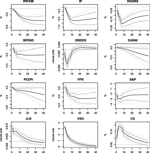
Figures 1 and 2 show the impulse responses to macro and financial uncertainty shocks, respectively. Uncertainty has a strong recessionary effect on employment, industrial production, hours worked, consumer spending and real manufacturers’ new orders; the financial conditions also deteriorate, as shown by the response of stock market and credit spreads. The fall in the federal funds rate is consistent with monetary policy trying to counteract the depressive effects of heightened uncertainty. Notably, shocks to macroeconomic uncertainty increase financial uncertainty, and vice-versa. Interestingly, we find some evidence in favor of a negative response of prices (using inflation rate provides similar results) for financial uncertainty shocks only; on the other hand, macro uncertainty does not seem to put any significant pressure on prices. This suggests that financial uncertainty disturbances mimic demand shocks, namely they trigger a recession and a deflationary pressure on the economy. The interpretation for macro uncertainty is more mixed.

Fig. 1 Responses to macroeconomic uncertainty shocks. The figure reports the posterior mean (black solid lines), the 68% Bayesian credibility region (black dashed lines), and the 90% Bayesian credibility region (gray dashed lines). The shock size is set to one standard deviation.

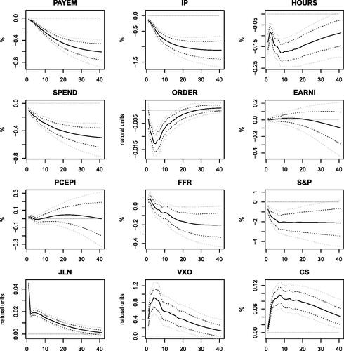
Fig. 2 Responses to financial uncertainty shocks. The figure reports the posterior mean (black solid lines), the 68% Bayesian credibility region (black dashed lines), and the 90% Bayesian credibility region (gray dashed lines). The shock size is set to one standard deviation.

Among others, Furlanetto, Ravazzolo, and Sarferaz (2017), Caldara et al. (2016), Caggiano et al. (2021), and Brianti (2021) stress the need to identify credit shocks and sharpen the identification of uncertainty shocks accordingly. Figure 3 shows that an increase in credit spreads has a depressive and deflationary effect on macroeconomic variables and leads to higher uncertainty, especially financial uncertainty. The fall of prices and the loose monetary policy are both more severe than what is induced by uncertainty shocks.

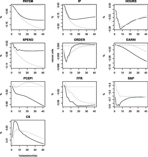
To facilitate comparisons, Figure 4 compares the impulse responses to macro and financial uncertainty shocks (by normalizing the shocks size to the same amount). The effects of macroeconomic and financial uncertainty are qualitatively different for prices (and earnings). Further quantitative differences arise. For example, the recessionary effect on real activity variables seem more pronounced following macroeconomic uncertainty shocks, while financial conditions deteriorate more with financial uncertainty shocks. In order to distinguish identified uncertainty shocks from other shocks, in supplemental Appendix D we (i) re-estimate the model by controlling for a series of demand and supply shocks, finding that the results are unchanged and (ii) show that the correlation between our identified uncertainty shocks and demand and supply shocks are not statistically significant.

Fig. 3 Responses to financial (credit supply) shocks. The figure reports the posterior mean (black solid lines), the 68% Bayesian credibility region (black dashed lines), and the 90% Bayesian credibility region (gray dashed lines). The shock size is set to one standard deviation.

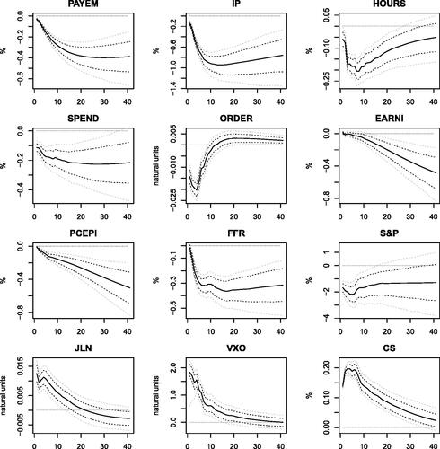
Fig. 4 Comparison between macro and financial uncertainty shocks. The gray and black line denote the posterior mean of the impulse response functions to macroeconomic and financial uncertainty shock, respectively. Size of the shocks has been normalized to 1%.

When re-estimating the responses without inequality constraints on the FEVD, we find that the results are qualitatively unchanged, but quantitative differences can raise (especially for the responses to the credit shocks and when the horizon of maximization is other than $\tilde{h}=5$).

4.3 Endogenous Uncertainty?

Since our scheme allows for a contemporaneous feedback effect from economic and financial variables to uncertainty, it provides a natural ground to look into the issue of endogeneity of uncertainty. In order to tackle this question, we look into the FEVD. Table 1 presents the FEVD of macroeconomic uncertainty proxy, financial uncertainty proxy, and credit spreads due to the three shocks of interest. It seems that uncertainty, especially macro uncertainty, is at least partially endogenous: the contribution of macro (financial) uncertainty shock to the FEV of JLN (VXO) is below 100%, suggesting that other shocks affect macro (financial) uncertainty. Considering estimation uncertainty (Bayesian credible intervals) does not change the overall picture, that is uncertainty, even contemporaneously, is never 100% exogenous.

Table 1 FEVD (%).

$u{F}^{*}$ shock	h = 0	h = 10	h = 20	h = 40
$u{F}^{*}$	91.63	10.64	6.39	4.46
$u{M}^{*}$	8.46	2.04	1.04	0.61
CS	9.57	3.86	1.90	1.04
$u{M}^{*}$ shock
$u{F}^{*}$	1.64	1.60	1.21	0.94
$u{M}^{*}$	86.81	10.05	5.25	2.95
CS	0.56	1.93	1.42	1.02
CS shock
$u{F}^{*}$	28.65	4.03	2.39	1.69
$u{M}^{*}$	7.48	2.01	0.97	0.62
CS	75.14	8.86	4.41	2.38

However, such a conclusion is debated in the literature. Ludvigson, Ma, and Ng (2021) argue that, while financial uncertainty is mainly exogenous, macroeconomic uncertainty presents some endogeneity. Angelini et al. (2019) find that both macroeconomic and financial uncertainty are mostly exogenous, and Carriero, Clark, and Marcellino (2021) point out that macroeconomic uncertainty displays some endogeneity, though more at quarterly than monthly frequency.

Each study above adopts a different identification strategy. Ludvigson, Ma, and Ng (2021) use a small-scale model and a set-identification approach based on narrative restrictions requiring the shocks to be consistent with some historical episodes and correlated with some external instruments. Instead, we use a large-scale model, which reduces the problems of possible omitted variable bias, and a point-identification approach, which avoids the problems inherent in set-identification discussed for example in Giacomini, Kitagawa, and Read (2021).

Angelini et al. (2019) also use a small-scale model in which there are no proxies for financial conditions. They achieve identification by assuming that in the sample preceding January 2008 financial uncertainty shocks could neither contemporaneously impact on nor been impacted by macro variables directly. However, an indirect channel on real variables through the impact from financial uncertainty to macro uncertainty is allowed since the Great Moderation. Differently from them, we never assume exogeneity of financial uncertainty, not even in some sub-samples, and we use a large-scale model which includes financial variables and a credit channel.

Carriero, Clark, and Marcellino (2021) employ a large model and achieve point-identification exploiting heteroscedasticity in the error terms of the SVAR. However, their framework does not include macroeconomic and financial uncertainty in the same unified setting. Furthermore, their approach requires an ordering restriction on the block of macroeconomic variables in which pure financial shocks are not explicitly identified. Instead, the approach of this article allows to identify shocks to financial and macroeconomic uncertainty which are orthogonal by construction, and to disentangle them from pure financial shocks.

5 Conclusions

This article developed a novel multiple shocks identification scheme for SVARs, based on generalizing the Max Share to joint identification of a multiplicity of shocks. Our approach overcomes some drawbacks induced by individually identified shocks, that is those shocks (i) tend to be correlated to each other or (ii) can be separated under orthogonalizations with weak economic ground. We characterized the properties of this approach, such as non-emptiness and point-identification, and provided an algorithm for its implementation. The toolkit developed in this article can be applied to any SVAR where standard ordering and sign restrictions are not desirable or sufficient to identify all of the shocks. We used the approach and U.S. data to investigate the effects of uncertainty (allowing for the possibility that uncertainty responds endogenously to other variables or shocks) and financial shocks. We found that financial uncertainty shocks mimic demand disturbances, while this is not the case for macro uncertainty. On the other hand, our results suggest that, while contemporaneous variation in uncertainty measures tends to be largely driven by uncertainty shocks, a nontrivial fraction of the variation in these measures is driven by other (non-uncertainty) shocks, particularly beyond short horizons.

Supplementary Materials

The Supplementary material consists of a Supplemental Appendix, data and codes. The Appendix contains omitted proofs (Appendix A), theory-driven justification of our approach applied to uncertainty and financial shocks (Appendix B), simulation exercises (Appendix C), robustness checks (Appendix D), algorithms for checking non-emptiness (Appendix E), representation in the frequency domain (Appendix F), generalization of the setting to (i) maximize the FEVD over (rather than at) a period of time (Appendix G) (ii) different timing for different shocks (Appendix H).

Acknowledgments

We thank the editor Professor Atsushi Inoue, an anonymous associate editor, and two anonymous referees. Their comments and suggestions considerably improved this article. We thank Toru Kitagawa, Ana Galvão, Valentina Corradi, Luca Fanelli, Marco Brianti, Robin Braun, Stepana Lazarova, MatthewRead, Martin Bruns and Kerem Tuzcuoglu for insightful suggestions. Volpicella gratefully acknowledges financial support the Royal Economic Society (Conference Grant, 2022). This article previously circulated with the title “Identification through the Forecast Error Variance Decomposition: an Application to Uncertainty,” and “Generalizing the Max Share Identification to multiple shocks identification: an Application to Uncertainty.”

Disclosure Statement

The authors report there are no competing interests to declare.

References

- Amir-Ahmadi, P., and Drautzburg, T. (2021), “Identification and Inference with Ranking Restrictions,” Quantitative Economics, 12, 1–39. DOI: 10.3982/QE1277.
- Angeletos, G.-M., Collard, F., and Dellas, H. (2020), “Business-cycle Anatomy,” American Economic Review, 110, 3030–3070. DOI: 10.1257/aer.20181174.
- Angelini, G., Bacchiocchi, E., Caggiano, G., and Fanelli, L. (2019), “Uncertainty across Volatility Regimes,” Journal of Applied Econometrics, 34, 437–455. DOI: 10.1002/jae.2672.
- Barsky, R. B., and Sims, E. R. (2011), “News Shocks and Business Cycles,” Journal of monetary Economics, 58, 273–289. DOI: 10.1016/j.jmoneco.2011.03.001.
- Baumeister, C., and Hamilton, J. D. (2015), “Sign Restrictions, Structural Vector Autoregressions, and Useful Prior Information,” Econometrica, 83, 1963–1999. DOI: 10.3982/ECTA12356.
- Berger, D., Dew-Becker, I., and Giglio, S. (2020), “Uncertainty Shocks as Second-Moment News Shocks,” The Review of Economic Studies, 87, 40–76. DOI: 10.1093/restud/rdz010.
- Blanchard, O. J., and Quah, D. (1989), “The Dynamic Effects of Aggregate Demand and Supply Disturbances,” American Economic Review, 79, 655–673.
- Bloom, N. (2009), “The Impact of Uncertainty Shocks,” Econometrica, 77, 623–685.
- ——- (2014), “Fluctuations in Uncertainty,” Journal of Economic Perspectives, 28, 153–76.
- Bollerslev, T., Tauchen, G., and Zhou, H. (2009), “Expected Stock Returns and Variance Risk Premia,” The Review of Financial Studies, 22, 4463–4492. DOI: 10.1093/rfs/hhp008.
- Bonciani, D., and Oh, J. (2022), “Uncertainty Shocks, Innovation, and Productivity,” The BE Journal of Macroeconomics, 23, 279–335. DOI: 10.1515/bejm-2021-0074.
- Brianti, M. (2021), “Financial Shocks, Uncertainty Shocks, and Monetary Policy Trade-Offs,” unpublished manuscript.
- Caggiano, G., Castelnuovo, E., Delrio, S., and Kima, R. (2021), “Financial Uncertainty and Real Activity: The Good, the Bad, and the Ugly,” European Economic Review, 136, 103750. DOI: 10.1016/j.euroecorev.2021.103750.
- Caldara, D., Fuentes-Albero, C., Gilchrist, S., and Zakrajšek, E. (2016), “The Macroeconomic Impact of Financial and Uncertainty Shocks,” European Economic Review, 88, 185–207. DOI: 10.1016/j.euroecorev.2016.02.020.
- Carrière-Swallow, Y., and Céspedes, L. F. (2013), “The Impact of Uncertainty Shocks in Emerging Economies,” Journal of International Economics, 90, 316–325. DOI: 10.1016/j.jinteco.2013.03.003.
- Carriero, A., Clark, T. E., and Marcellino, M. (2021), “Using Time-Varying Volatility for Identification in Vector Autoregressions: An Application to Endogenous Uncertainty,” Journal of Econometrics, 225, 47–73. DOI: 10.1016/j.jeconom.2021.07.001.
- Cascaldi-Garcia, D., and Galvão, A. B. (2021), “News and Uncertainty Shocks,” Journal of Money, Credit and Banking, 4, 779–811. DOI: 10.1111/jmcb.12727.
- Cerra, V., and Saxena, S. C. (2008), “Growth Dynamics: The Myth of Economic Recovery,” American Economic Review, 98, 439–457. DOI: 10.1257/aer.98.1.439.
- DiCecio, R., and Owyang, M. (2010), “Identifying Technology Shocks in the Frequency Domain,” Federal Reserve Bank of St. Louise Working Paper No 2010-025A.
- Dieppe, A., Francis, N., and Kindberg-Hanlon, G. (2021), “The Identification of Dominant Macroeconomic Drivers: Coping with Confounding Shocks,” ECB working paper no. 2021/2534.
- Francis, N., Owyang, M. T., Roush, J. E., and DiCecio, R. (2014), “A Flexible Finite-Horizon Alternative to Long-Run Restrictions with an Application to Technology Shocks,” Review of Economics and Statistics, 96, 638–647. DOI: 10.1162/REST_a_00406.
- Furlanetto, F., Ravazzolo, F., and Sarferaz, S. (2017), “Identification of Financial Factors in Economic Fluctuations,” The Economic Journal, 129, 311–337. DOI: 10.1111/ecoj.12520.
- Gafarov, B., Meier, M., and Olea, J. L. M. (2018), “Delta-Method Inference for a Class of Set-Identified SVARs,” Journal of Econometrics, 203, 316–327. DOI: 10.1016/j.jeconom.2017.12.004.
- Giacomini, R., and Kitagawa, T. (2021), “Robust Bayesian Inference for Set-Identified Models,” Econometrica, 89, 1519–1556. DOI: 10.3982/ECTA16773.
- Giacomini, R., Kitagawa, T., and Read, M. (2021), “Identification and Inference under Narrative Restrictions,” arXiv:2102.06456.
- ——- (2022), “Robust Bayesian Inference in Proxy SVARs,” Journal of Econometrics, 228, 107–126.
- Giacomini, R., Kitagawa, T., and Volpicella, A. (2022), “Uncertain Identification,” Quantitative Economics, 13, 95–123. DOI: 10.3982/QE1671.
- Giannone, D., Lenza, M., and Reichlin, L. (2019), “Money, Credit, Monetary Policy, and the Business Cycle in the Euro Area: What Has Changed Since the Crisis?” International Journal of Central Banking, 15, 137–173.
- Granziera, E., Moon, H. R., and Schorfheide, F. (2018), “Inference for VARs Identified with Sign Restrictions,” Quantitative Economics, 9, 1087–1121. DOI: 10.3982/QE978.
- Jurado, K., Ludvigson, S. C., and Ng, S. (2015), “Measuring Uncertainty,” American Economic Review, 105, 1177–1216. DOI: 10.1257/aer.20131193.
- Kilian, L., and Murphy, D. (2012), “Why Agnostic Sign Restrictions Are Not Enough: Understanding the Dynamics of Oil Market VAR Models,” Journal of the European Economic Association, 10, 1166–1188. DOI: 10.1111/j.1542-4774.2012.01080.x.
- Kurmann, A., and Sims, E. (2021), “Revisions in Utilization-Adjusted TFP and Robust Identification of News Shocks,” The Review of Economics and Statistics, 103, 216–235. DOI: 10.1162/rest_a_00896.
- Levchenko, A. A., and Pandalai-Nayar, N. (2020), “TFP, News, and “Sentiments”: The International Transmission of Business Cycles,” Journal of the European Economic Association, 18, 302–341. DOI: 10.1093/jeea/jvy044.
- Ludvigson, S., Ma, S., and Ng, S. (2021), “Uncertainty and Business Cycles: Exogenous Impulse or Endogenous Response?” American Economic Journal: Macroeconomics, 13, 369–410. DOI: 10.1257/mac.20190171.
- Mertens, K., and Ravn, M. O. (2013), “The Dynamic Effects of Personal and Corporate Income Tax Changes in the United States,” American Economic Review, 103, 1212–1247. DOI: 10.1257/aer.103.4.1212.
- Mumtaz, H., Pinter, G., and Theodoridis, K. (2018), “What do VARs tell US about the Impact of a Credit Supply Shock?” International Economic Review, 59, 625–646. DOI: 10.1111/iere.12282.
- Mumtaz, H., and Theodoridis, K. (2023), “The Federal Reserve’s Implicit Inflation Target and Macroeconomic Dynamics. A SVAR Analysis,” International Economic Review, forthcoming. DOI: 10.1111/iere.12638.
- Ng, S., and Wright, J. H. (2013), “Facts and Challenges from the Great Recession for Forecasting and Macroeconomic Modeling,” Journal of Economic Literature, 51, 1120–54. DOI: 10.1257/jel.51.4.1120.
- Piffer, M., and Podstawski, M. (2018), “Identifying Uncertainty Shocks Using the Price of Gold,” The Economic Journal, 128, 3266–3284. DOI: 10.1111/ecoj.12545.
- Shin, M., and Zhong, M. (2020), “A New Approach to Identifying the Real Effects of Uncertainty Shocks,” Journal of Business & Economic Statistics, 38, 367–379. DOI: 10.1080/07350015.2018.1506342.
- Sims, C. (1980), “Macroeconomics and Reality,” Econometrica, 48, 1–48. DOI: 10.2307/1912017.
- Uhlig, H. (2004), “What Moves GNP?” in Econometric Society 2004 North American Winter Meeting, number 636. Econometric Society.
- ——- (2005), “What Are the Effects of Monetary Policy on Output? Results from an Agnostic Identification Procedure,” Journal of Monetary Economics, 52, 381–419.
- Uhlig, H. (2017), “Shocks, Sign Restrictions, and Identification,” in Advances in Economics and Econometrics (Vol. 2), eds. M. B. Honore, A. Pakes, and L. Samuelson, pp. 95–127, Cambridge: Cambridge University Press.
- Volpicella, A. (2022), “SVARs Identification through Bounds on the Forecast Error Variance,” Journal of Business & Economic Statistics, 40, 1291–1301. DOI: 10.1080/07350015.2021.1927742.