Gamma-Driven Markov Processes and Extensions with Application to Realized Volatility

Abstract

We propose a novel class of Markov processes for dealing with continuous positive time series data, which is constructed based on a latent gamma effect and named gamma-driven (GD) models. The GD processes possess desirable properties and features: (i) it can produce any desirable invariant distribution with support on ${\mathbb{R}}^{+}$, (ii) it is time-reversible, and (iii) it has the transition density function given in an explicit form. Estimation of parameters is performed through the maximum likelihood method combined with a Gauss Laguerre quadrature to approximate the likelihood function. The evaluation of the estimators and also confidence intervals of parameters are explored via Monte Carlo simulation studies. Two generalizations of the GD processes are also proposed to handle nonstationary and long-memory time series. We apply the proposed methodologies to analyze the daily realized volatility of the FTSE 100 equity index.

KEYWORDS:

• Gauss Laguerre quadrature
• Generalized inverse-Gaussian distribution
• Positive continuous time series
• Stationarity
• Time-reversible processes
• Weight gamma density

1 Introduction

In stochastic process theory and application, there is extensive literature about the construction of Markov processes. More than being well adjustable to the data, desirable properties like stationarity and reversibility in time are sometimes required. In time series, there is solid literature on this type of construction. The classic AR(1) model is one of the most famous and defined by a sequence of random variables ${\left\{X_t\right\}}_{t\in \mathbb{Z}}$ satisfying $$X_t=\rho X_{t-1}+{ϵ}_t,$$where ${\left\{{ϵ}_t\right\}}_{t\in \mathbb{Z}}$ are independent and identically distributed random variables (iid) with zero mean and variance ${\sigma }^2$ and independent of $(X_{t-1},X_{t-2},\dots )$ and $\rho \in \mathbb{R}$.

Outside the scenario where normality is assumed, establishing the distribution of ${\left\{{ϵ}_t\right\}}_{t\in \mathbb{Z}}$ such that the strict stationarity of ${\left\{X_t\right\}}_{t\in \mathbb{Z}}$ is guaranteed is a challenging task. Some authors fixed this issue by dealing directly with the marginal of the model, ensuring that the results of interest were satisfied. Jacobs and Lewis (1977) and Lawrance and Lewis (1977) proposed the construction of first-order autoregressive processes with exponential marginals. Gaver and Lewis (1980), in turn, explored the properties of first-order autoregressive processes whose marginal followed a gamma distribution (for $0\le \rho <1$).

Joe (1980) made significant advances by proposing time series models with the distribution of the response variable X_t belonging to an infinitely divisible class closed by convolution. The class includes the Poisson, negative binomial (with fixed probability parameter), gamma (with fixed scale parameter), Generalized Poisson (with one fixed parameter), inverse-Gaussian (with one fixed parameter), and normal distributions. Among the models proposed by Joe (1980), there is a stationary and time-reversible AR(1) Markov model. There is vast literature about Markov process constructions with discrete marginal. For example, the integer-valued autoregressive (INAR) processes introduced by McKenzie (1985) and Al-Osh and Alzaid (1987).

Pitt, Chatfield, and Walker (2002) introduce an alternative way to the ones mentioned above to build first-order autoregressive models. The construction of the process is done by specifying the joint density of $(X_{t-1},X_t)$, or equivalently, specifying the marginal distribution of X_t and the conditional (transition) of $X_t|X_{t-1}$. Mena and Walker (2005) proposed the construction of a Markov process with a nonparametric approach to model the transition density with desirable stationary densities. A generalization of this nonparametric approach with a focus on the discrete case was considered by Contreras-Cristán, Mena, and Walker (2009).

Following this same line of construction, Anzarut et al. (2018) proposed a method for constructing strictly stationary Markov models, which have a similar structure to the models by Pitt, Chatfield, and Walker (2002) and Mena and Walker (2005). Their processes are driven by a Poisson transformation, which modulates their dependency structure. The construction allows for time-reversibility and stationarity with the desirable invariant distribution of interest. Further, the authors considered a Bayesian approach to make inference. Leisen et al. (2019) proposed construction of stationary Markov models having negative binomial marginals. They showed that choosing the negative binomial distribution as marginal leads them to find analytical conditions that satisfy the Chapman-Kolmogorov equations leading to a rich class of continuous-time Markov chains. Using their conditional probability structure, Palma and Mena (2021) proposed a dual continuous-time Markov process.

Our chief aim in this article is to propose a novel way to construct stationary Markov processes having any desirable positive continuous distribution in the marginals. To do that, we introduce a weighted gamma density function, which will control the dependence structure within our class of time series models. We call our class the gamma-driven (GD) Markov processes. We show that simple expressions can be found for the transition densities and autocorrelation. The GD models can be seen as an alternative to the Poisson-driven (PD) models by Anzarut et al. (2018). In particular, we show through an empirical illustration that our GD processes can have a better predictive power than PD processes for modeling realized volatility. Another key contribution of our article is the proposal of two generalizations of GD models to handle nonstationary and long-memory time series.

We apply the proposed gamma-driven models to analyze the daily realized volatility of FTSE 100 equity index log-returns computed every 10 min from October 31st, 2003, to May 31st, 2007. In an initial study under this “short” period of time, we compare our GD models with the Poisson-driven approach through out-of-sample prediction exercises. Our findings show that our models produce better predictions than Poisson-driven models for the realized volatility considered. In a second study, we consider the daily realized volatility of FTSE 100 for a longer period of time, from January 2nd, 2004 to December 4th, 2017. To handle this problem, an extension of the GD processes is developed to accommodate long memory, which is a feature commonly observed in the analysis of realized volatility. Our results reveal that such an extension is needed and yields better predictions when compared to the Markovian GD models.

The article is organized as follows. Section 2 deals with the construction of the gamma-driven (GD) Markov processes. Some properties of the GD models are established, such as time-reversibility and stationarity. Further, the cases where the marginals are gamma and inverse-Gaussian distributed are explored in more detail. Section 3 deals with maximum likelihood estimation combined with Gauss Laguerre quadrature to approximate the log-likelihood function. Furthermore, Monte Carlo simulations are presented to evaluate the performance of the proposed estimation procedure. We propose two generalizations of the GD processes to handle nonstationary and long-memory time series in Section 4. Section 5 illustrates the usefulness of our methodology, where the daily realized volatility of the FTSE 100 index log-returns is analyzed. Concluding remarks and possible future research are provided in Section 6. This article contains supplementary materials.

2 Gamma-Driven Markov Processes

We introduce the weighted gamma density function, which will play an important role in constructing the stationary gamma-driven Markov processes. A random variable Z following a gamma distribution with shape and scale parameters $\mathrm{(}\text{HTML translation failed}\mathrm{)}$ and $\beta >0$, respectively, is denoted by $Z\sim \text{Ga}(\alpha ,\beta )$ and has density function given by $g(z)=\frac{{\beta }^{\alpha }}{\Gamma (\alpha )}{z}^{\alpha -1}{e}^{-\beta z}$, for z > 0.

Definition 2.1.

(Weighted gamma density) Let X be a positive continuous random variable with density function f, and assume that Y is a random variable such that $Y|X=x\sim \text{Ga}(\varphi ,x)$, for $\varphi >0$. The weighted gamma density function is defined as the conditional density of $X|Y=y$, which assumes the form (1) $$\widehat{f}(x;y,\varphi )=\frac{x^{\varphi }{e}^{-\mathit{\text{xy}}}f(x)}{\eta (y,\varphi )},$$(1)

where $\eta (·,·)$ is the normalization constant (2) $$\eta (y,\varphi )={\int }_0^{\infty }{x}^{\varphi }{e}^{-\mathit{\text{xy}}}f(x)\mathit{\text{dx}}.$$(2)

If $X|Y=y$ has a conditional probability density function given in (1), the associated rth moment and Laplace transform are respectively given by (3) $$\begin{array}{c}E(X^r|Y=y)=\frac{\eta (y,r+\varphi )}{\eta (y,\varphi )}\hspace{1em}\text{and}\\ E(e^{-\mathit{\text{sX}}}|Y=y)=\frac{\eta (y+s,\varphi )}{\eta (y,\varphi )},\hspace{1em}s>0.\end{array}$$(3)

Let ${\left\{X_t\right\}}_{t\in \mathbb{N}}$ be a stationary stochastic process with arbitrary marginal density f with support on ${\mathbb{R}}_{+}$. Using the idea on weighted gamma densities above, we consider a latent stochastic process ${\left\{Y_t\right\}}_{t\in \mathbb{N}}$ such that $Y_t|X_t=x_t\sim \text{Ga}(\varphi ,x_t)$ and then $X_t|Y_{t-1}=y$ has a gamma weighted density function given in (1), for $t\in \mathbb{N}$. Under the above construction, we obtain that the conditional density function of X_t given $X_{t-1}=x_{t-1}$ (transition density) is (4) $$\begin{array}{c}f(x_t|x_{t-1})={\int }_0^{\infty }\widehat{f}(x_t;y,\varphi )\frac{x_{t-1}^{\varphi }{y}^{\varphi -1}{e}^{x_{t-1}y}}{\Gamma (\varphi )}\mathit{\text{dy}}\\ =\frac{{(x_t{x}_{t-1})}^{\varphi }f(x_t)}{\Gamma (\varphi )}{\int }_0^{\infty }\frac{e^{-y(x_t+x_{t-1})}{y}^{\varphi -1}}{\eta (y,\varphi )}\mathit{\text{dy}}.\end{array}$$(4)

Definition 2.1. We say that a stochastic process in discrete-time ${\left\{X_t\right\}}_{t\in \mathbb{N}}$ is a stationary gamma-driven (GD) Markov process if its density transitions are given by (4), for some density function f with support on ${\mathbb{R}}_{+}$.

We now show that a GD process is stationary and time-reversible. Therefore, the above method gives us one way to construct stationary Markov processes with any desirable positive continuous distribution in the marginals.

Proposition 2.2.

The gamma-driven processes are stationary and time-reversible.

Proof.

Let ${\left\{X_t\right\}}_{t\in \mathbb{N}}$ be a GD process. From (4), we have that (5) $$\begin{array}{c}f(x_t|x_{t-1})f(x_{t-1})=\frac{{(x_t{x}_{t-1})}^{\varphi }f(x_t)}{\Gamma (\varphi )}{\int }_0^{\infty }\frac{e^{-y(x_t+x_{t-1})}{y}^{\varphi -1}}{\eta (y,\varphi )}\mathit{\text{dyf}}(x_{t-1})\\ =f(x_{t-1}|x_t)f(x_t),\end{array}$$(5) for all $x_t,x_{t-1}>0$. In other words, the process satisfies the detailed balance equation and is therefore time-reversible. Using (4) again, it follows that (6) $$\begin{array}{c}{\int }_0^{\infty }f(x_t,x_{t-1})d{x}_{t-1}={\int }_0^{\infty }f(x_{t-1})\frac{{(x_t{x}_{t-1})}^{\varphi }f(x_t)}{\Gamma (\varphi )}\\ \hspace{1em}\times ({\int }_0^{\infty }\frac{e^{-y(x_t+x_{t-1})}{y}^{\varphi -1}}{\eta (y,\varphi )}\mathit{\text{dy}})d{x}_{t-1}\\ =f(x_t).\end{array}$$(6)

Hence, ${\left\{X_t\right\}}_{t\in \mathbb{N}}$ is a stationary process with marginal densities f. □

We now provide an expression for the conditional moments of the GD processes. These moments will be used to obtain the lag-1 autocorrelation of our Markov models.

Proposition 2.3.

Let ${\left\{X_t\right\}}_{t\in \mathbb{N}}$ be a GD process. For $t\ge 2$, the rth conditional moment of X_t given $X_{t-1}=x_{t-1}$ can be expressed by (7) $$\mathbf{E}(X_t^r|X_{t-1}=x_{t-1})=\frac{x_{t-1}^{\varphi }}{\Gamma (\varphi )}{\int }_0^{\infty }\frac{\eta (y,\varphi +r)y^{\varphi -1}{e}^{-x_{t-1}y}}{\eta (y,\varphi )}\mathit{\text{dy}}.$$(7)

Proof.

For $r\in \mathbb{N}$ and using (3) and (4), we obtain that rth conditional moment X_t given $X_{t-1}=x_{t-1}$ is given by $$\begin{array}{c}\mathbf{E}(X_t^r|X_{t-1}=x_{t-1})={\int }_0^{\infty }{x}_t^{r}f(x_t|x_{t-1})d{x}_t\\ ={\int }_0^{\infty }{x}_t^r{\int }_0^{\infty }\widehat{f}(x_t;y,\varphi )\frac{x_{t-1}^{\varphi }{y}^{\varphi -1}{e}^{-x_{t-1}y}}{\Gamma (\varphi )}\mathit{\text{dyd}}{x}_t\\ ={\int }_0^{\infty }\frac{x_{t-1}^{\varphi }{y}^{\varphi -1}{e}^{-x_{t-1}y}}{\Gamma (\varphi )\eta (y,\varphi )}{\int }_0^{\infty }{x}_t^{\varphi +r}{e}^{-x_{t}y}f(x_t)d{x}_t\mathit{\text{dy}}\\ ={\int }_0^{\infty }\frac{\eta (y,\varphi +r)x_{t-1}^{\varphi }{y}^{\varphi -1}{e}^{-x_{t-1}y}}{\eta (y,\varphi )\Gamma (\varphi )}\mathit{\text{dy}}.\end{array}$$

□

If the density function f is square integrable, we can use the above result to get that the lag-1 autocorrelation of a GD process can be expressed by (8) $$\text{corr}(X_t,X_{t-1})=\frac{1}{{\sigma }^2}(\frac{1}{\Gamma (\varphi )}{\int }_0^{\infty }\frac{y^{\varphi -1}{\eta }^2(y,\varphi +1)}{\eta (y,\varphi )}\mathit{\text{dy}}-{\mu }^2),$$(8) where $\mu ={\int }_0^{\infty }xf(x)\mathit{\text{dx}}$ and ${\sigma }^2={\int }_0^{\infty }{(x-\mu )}^{2}f(x)\mathit{\text{dx}}$ are respectively the mean and variance associated with the density f. The parameter ϕ controls the model dependence. This will be illustrated in the next sections, where we explore two special cases of the GD models.

2.1 Generalized Inverse-Gaussian GD Process

In this section, we consider the GD model having generalized inverse-Gaussian marginals (in short, GIG-GD). A random variable X following a GIG distribution with parameters $\beta \in \mathbb{R},\delta >0$ and $\gamma >0$ is denoted by $X\sim \text{GIG}(\beta ,\delta ,\gamma )$ and has probability density function given by (9) $$f(x)=\frac{{(\gamma /\delta )}^{\frac{\beta }{2}}}{2K_{\beta }\left(\sqrt{\delta \gamma }\right)}{x}^{\beta -1}{e}^{-\frac{1}{2}(\delta x^{-1}+\gamma x)},\hspace{1em}x>0,$$(9) where $K_{\beta }(u)=\frac{1}{2}{\int }_0^{\infty }{x}^{\beta -1}{e}^{-\frac{1}{2}u(x+x^{-1})}\mathit{\text{dx}}$ is the modified Bessel function of the third kind with index β; for instance, see Abramowitz and Stegun (1974).

By identifying a GIG kernel density, it can be shown that the normalized constant $\eta (·,·)$ in (2) is (10) $$\eta (y,\varphi )=\frac{{(\delta /(\gamma +2y))}^{\frac{\beta +\varphi }{2}}{K}_{\beta +\varphi }(\sqrt{\delta (\gamma +2y)})}{{(\delta /\gamma )}^{\frac{\beta }{2}}{K}_{\beta }\left(\sqrt{\delta \gamma }\right)}.$$(10)

Hence, using expression (10) and considering f a density function as in (9), we obtain that the weighted gamma density function $\widehat{f}$ assumes the form (11) $$\widehat{f}(x;y,\varphi )=\frac{x^{\varphi +\beta -1}\hspace{0.17em}\mathrm{\text{exp}}\hspace{0.17em}\{-\frac{1}{2}(\delta x^{-1}+(\gamma +2y)x)\}}{{(\delta /(\gamma +2y))}^{\frac{\beta +\varphi }{2}}{K}_{\beta +\varphi }(\sqrt{\delta (\gamma +2y)})},\hspace{1em}x>0.$$(11)

Note that the conditional distribution associated with the density in (11) is $\text{GIG}(\varphi +\beta ,\delta ,\gamma +2y)$. Let ${\left\{X_t\right\}}_{t\in \mathbb{N}}$ be a GIG-GD process. Then, its transition densities can be expressed as $$\begin{array}{c}f(x_t|x_{t-1})=\frac{{(x_t{x}_{t-1})}^{\varphi }{x}_t^{\beta -1}\hspace{0.17em}\mathrm{\text{exp}}\hspace{0.17em}\left\{-\frac{1}{2}(\delta x_t^{-1}+\gamma x_t)\right\}}{2{\delta }^{\frac{\varphi +\beta }{2}}\Gamma (\varphi )}\\ \times {\int }_0^{\infty }\frac{{(\gamma +2y)}^{\frac{\varphi +\beta }{2}}{e}^{-y(x_t+x_{t-1})}{y}^{\varphi -1}}{K_{\beta +\varphi }(\sqrt{\delta (\gamma +2y)})}\mathit{\text{dy}},\end{array}$$for $x_t>0$ and $t\ge 2$. The conditional expectation of X_t given $X_{t-1}=x_{t-1}$ is of interest to perform prediction or forecasting. From (7), we obtain that (12) $$\mathbb{E}(X_t|X_{t-1})=\frac{x_{t-1}^{\varphi }{\delta }^{\frac{1}{2}}}{\Gamma (\varphi )}{\int }_0^{\infty }\frac{y^{\varphi -1}{e}^{-x_{t-1}y}}{{(\gamma +2y)}^{\frac{1}{2}}}\frac{K_{\beta +\varphi +1}(\sqrt{\delta (\gamma +2y)})}{K_{\beta +\varphi }(\sqrt{\delta (\gamma +2y)})}\mathit{\text{dy}}.$$(12)

An expression for the 1-lag autocorrelation of the GIG-GD process can also be obtained by using (8) as follows: (13) $$\begin{array}{c}\text{corr}(X_t,X_{t-1})=\frac{{\gamma }^{\frac{\beta }{2}+1}{\delta }^{\frac{\varphi }{2}}{K}_{\beta }\left(\sqrt{\delta \gamma }\right)}{\Gamma (\varphi )(K_{\beta }(\sqrt{\delta \gamma }\left)K_{\beta +2}\right(\sqrt{\delta \gamma })-K_{\beta +1}^2(\sqrt{\delta \gamma }))}\\ \times {\int }_0^{\infty }\frac{K_{\varphi +\beta +1}^2(\sqrt{\delta (\gamma +2y)})y^{\varphi -1}}{{(\gamma +2y)}^{\frac{\varphi +\beta }{2}+1}{K}_{\varphi +\beta }(\sqrt{\delta (\gamma +2y)})}\mathit{\text{dy}}\\ -\frac{K_{\beta +1}^2\left(\sqrt{\delta \gamma }\right)}{K_{\beta +2}\left(\sqrt{\delta \gamma }\right)K_{\beta }\left(\sqrt{\delta \gamma }\right)-K_{\beta }^2\left(\sqrt{\delta \gamma }\right)}.\end{array}$$(13)

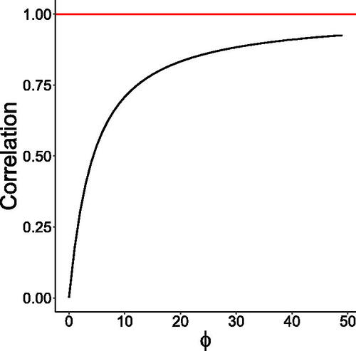
Figure 1 shows a plot of the lag-1 autocorrelation (13) as a function of ϕ for the GD model with marginals $\text{GIG}(1,2,3)$ distributed. The correlation between X_t and $X_{t-1}$ increases as ϕ increases and goes to zero when ϕ approaches zero.

Fig. 1 Plot of the lag-1 autocorrelation (13) as a function of ϕ for β = 1, δ = 2, and γ = 3.

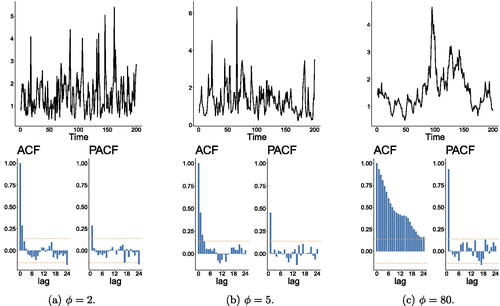
In Figure 2, we provide plots of simulated trajectories of the GIG-GD model with sample size n = 200 and their associated autocorrelation function (ACF) and partial autocorrelation function (PACF) plots for $(\beta ,\delta ,\gamma )=(1,2,3)$ and some values of ϕ. We can observe that the model seems to behave nonstationary when ϕ is large.

Fig. 2 Simulated trajectories of the GIG-GD process with marginals $\text{GIG}(1,2,3)$ distributed and their associated ACF and PACF plots for $\varphi =2,5$ and 80 and sample size 200.

2.2 Gamma GD Process

We now discuss the special case when the GD process has $\text{Ga}(a,b)$ marginals, where a > 0 and b > 0 are shape and scale parameters from a gamma distribution, respectively. The normalizing constant (2) is obtained for the gamma case by identifying a gamma kernel. More specifically, we have that $$\eta (y,\varphi )=\frac{b^a\Gamma (\varphi +a)}{\Gamma (a){(b+y)}^{\varphi +a}},\hspace{1em}y>0.$$

It can be checked that the associated weighted gamma density is $\text{Ga}(\varphi +a,b+y)$ distributed. Let ${\left\{X_t\right\}}_{t\in \mathbb{N}}$ be a GD process with $\text{Ga}(a,b)$ marginals. Then, its transition densities assume (14) $$\begin{array}{c}f(x_t|x_{t-1})=\frac{{(x_t{x}_{t-1})}^{\varphi }{x}_{t-1}^{a-1}{e}^{-b{x}_{t-1}}}{\Gamma (\varphi )\Gamma (\varphi +a)}\times \\ \text{}{\int }_0^{\infty }\mathrm{}\mathrm{}\mathrm{}{e}^{-y(x_t+x_{t-1})}{y}^{\varphi -1}{(b+y)}^{\varphi +a}\mathit{\text{dy}},\hspace{1em}\text{}{x}_t\mathrm{}>\mathrm{}0.\end{array}$$(14)

The conditional expectation and the lag-1 autocorrelation for the Gamma-GD process are given, respectively, by (15) $$\mathbb{E}(X_t|X_{t-1}=x_{t-1})=\frac{x_{t-1}^{\varphi }\Gamma (\varphi +a+1)}{\Gamma (\varphi )\Gamma (\varphi +a)}{\int }_0^{\infty }\frac{y^{\varphi -1}{e}^{-x_{t-1}y}}{(b+y)}\mathit{\text{dy}}$$(15)

and (16) $$\text{corr}(X_t,X_{t-1})=\frac{\varphi }{\varphi +a+1}.$$(16)

Note that we obtain an explicit and simple expression for the lag-1 autocorrelation. This also happens with the gamma Poisson-driven process by Anzarut et al. (2018). Another remarkable point is that the autocorrelation in our gamma model is by ϕ and also by the parameter a, related to the marginal distribution. For the gamma model by Anzarut et al. (2018), the lag-1 autocorrelation is just controlled by the parameter related to the latent Poisson variable.

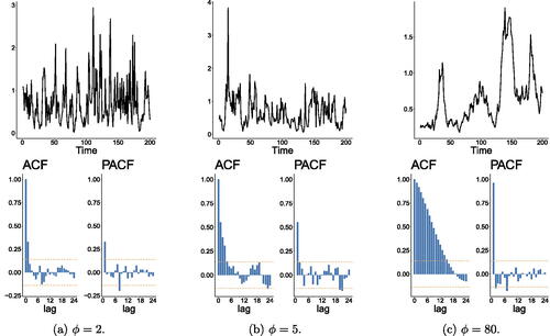
The autocorrelation (16) goes to 0 and 1 when ϕ tends to 0 and $\infty$, respectively. Figure 3 shows a plot of this function. We present plots of simulated trajectories, ACF, and PACF for the Gamma-GD process in Figure 4. Similarly, as in the GIG case, the simulated trajectory for the gamma case with $\varphi =80$ behaves like a nonstationary time series, which is suitable since $\text{corr}(X_t,X_{t-1})$ tends to 1 when $\varphi \to \infty$.

Fig. 3 Plot of the lag-1 autocorrelation (16) as a function of ϕ for a = 2.

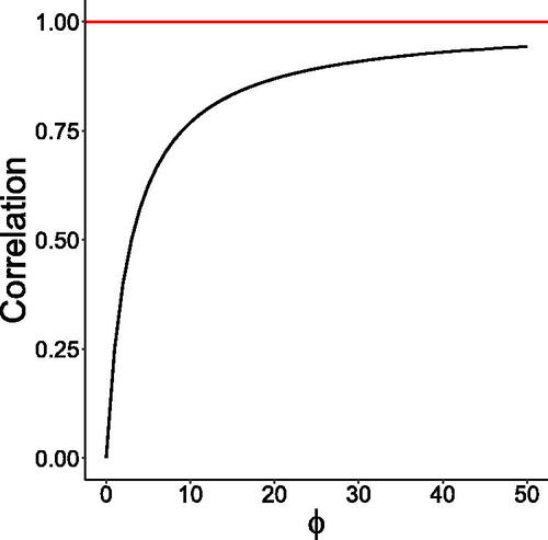
Fig. 4 Simulated trajectories of the Gamma-GD process with marginals $\text{Ga}(2,3)$ distributed and their associated ACF and PACF plots for $\varphi =2,5$, and 80 and sample size 200.

3 Parameter Estimation

We develop an estimation of the parameters of the GD processes through maximum likelihood estimation (MLE). We discuss the special cases where the marginals are gamma and GIG distributed. Denote by $x_1,\dots ,x_n$ an observed trajectory, and ${\theta }_1={(\varphi ,\beta ,\delta ,\gamma )}^{\top }$ and ${\theta }_2={(\varphi ,a,b)}^{\top }$ the vectors of parameters associated to the GIG-GD and Gamma-GD processes, respectively. The log-likelihood functions of the GIG and gamma cases are respectively given by (17) $$\begin{array}{c}\mathcal{l}({\theta }_1)=\sum _{i=2}^n[(\varphi +\beta -1)\hspace{0.17em}\mathrm{\text{log}}\hspace{0.17em}(x_i)+\varphi \hspace{0.17em}\mathrm{\text{log}}\hspace{0.17em}(x_{i-1})]\\ -\frac{1}{2}\sum _{i=2}^n(\delta x_i^{-1}+\gamma x_i)-(n-1)\hspace{0.17em}\mathrm{\text{log}}\hspace{0.17em}(\Gamma (\varphi ))\\ -\frac{(n-1)(\varphi +\beta )}{2}\mathrm{\text{log}}\hspace{0.17em}(\delta )\\ +\sum _{i=2}^n\hspace{0.17em}\mathrm{\text{log}}\hspace{0.17em}{\int }_0^{\infty }\frac{e^{-y(x_i+x_{i-1})}{y}^{\varphi -1}{(\gamma +2y)}^{(\varphi +\beta )/2}}{2K_{\varphi +\beta }(\sqrt{\delta (\gamma +2y)})}\mathit{\text{dy}}\\ +\frac{\beta }{2}\mathrm{\text{log}}\hspace{0.17em}(\gamma )-\frac{\beta }{2}\mathrm{\text{log}}\hspace{0.17em}(\delta )-\hspace{0.17em}\mathrm{\text{log}}\hspace{0.17em}(2)-\hspace{0.17em}\mathrm{\text{log}}\hspace{0.17em}(K_{\beta }(\sqrt{\delta \gamma }))\\ +(\beta -1)\hspace{0.17em}\mathrm{\text{log}}\hspace{0.17em}(x_1)-\frac{1}{2}(\delta x_1^{-1}+\gamma x_1)\end{array}$$(17)

and (18) $$\begin{array}{c}\mathcal{l}({\theta }_2)=\sum _{i=2}^n[(\varphi +a-1)\hspace{0.17em}\mathrm{\text{log}}\hspace{0.17em}(x_i)+\varphi \hspace{0.17em}\mathrm{\text{log}}\hspace{0.17em}(x_{i-1})]\\ -b\sum _{i=2}^n{x}_i-(n-1)\hspace{0.17em}\mathrm{\text{log}}\hspace{0.17em}(\Gamma (\varphi ))-(n-1)\hspace{0.17em}\mathrm{\text{log}}\hspace{0.17em}(\Gamma (\varphi +a))\\ +\sum _{i=2}^n\hspace{0.17em}\mathrm{\text{log}}\hspace{0.17em}{\int }_0^{\infty }{e}^{-y(x_i+x_{i-1})}{y}^{\varphi -1}{(b+y)}^{\varphi +a}\mathit{\text{dy}}+\\ a\hspace{0.17em}\mathrm{\text{log}}\hspace{0.17em}(b)-\hspace{0.17em}\mathrm{\text{log}}\hspace{0.17em}(\Gamma (a))+(a-1)\hspace{0.17em}\mathrm{\text{log}}\hspace{0.17em}(x_1)-b{x}_1.\end{array}$$(18)

The maximum likelihood estimators of the GIG-GD and Gamma-GD models are obtained by maximizing the log-likelihood functions (17) and (18), respectively. In both cases, we need to handle integrals. To tackle this problem, we propose an approximation for the integral through the numerical quadrature of Gauss Laguerre presented in Kahaner, Moler, and Nash (1989). The authors claim that certain functions usually appear as part of the integrand in infinite intervals and point out that two common cases are the functions $\hspace{0.17em}\mathrm{\text{exp}}\hspace{0.17em}\{-x\}$ and $\hspace{0.17em}\mathrm{\text{exp}}\hspace{0.17em}\{-x^2\}$. The method presented by the authors is based on the technique of weight functions. In particular, we have that approximation $${\int }_c^d{e}^{-x}h(x)\mathit{\text{dx}}=\sum _{k=1}^m{w}_{k}h(x_k)+R_n,$$where $h(·)$ is some function defined on the interval (c, d), the limits c and d can be finite or infinite, the points x_k are called nodes, while w_k are the weights associated with the nodes, and R_n denotes the rest; for more detail, please see Kahaner, Moler, and Nash (1989).

To approximate the integrals involved in the log-likelihood function, we use the gaussLaguerre function of the R package pracma with 17 weights and 17 nodes of the Gauss Laguerre Quadrature. The approximations to the integrals involved in the log-likelihoods (17) and (18) using Gauss Laguerre quadrature are (19) $$\begin{array}{c}{\int }_0^{\infty }\frac{e^{-y(x_i+x_{i-1})}{y}^{\varphi -1}{(\gamma +2y)}^{(\varphi +\beta )/2}}{2K_{\varphi +\beta }(\sqrt{\delta (\gamma +2y)})}\mathit{\text{dy}}\\ \hspace{1em}={\int }_0^{\infty }\frac{e^{-z}{\left(\frac{z}{x_i+x_{i-1}}\right)}^{\varphi -1}{\left(\gamma +\frac{2z}{x_i+x_{i-1}}\right)}^{(\varphi +\beta )/2}}{2K_{\varphi +\beta }\left(\sqrt{\delta \left(\gamma +\frac{2z}{x_i+x_{i-1}}\right)}\right)(x_i+x_{i-1})}\mathit{\text{dz}}\\ \hspace{1em}\approx \sum _{k=1}^{17}{w}_k\frac{{\left(\frac{z_k}{x_i+x_{i-1}}\right)}^{\varphi -1}{\left(\gamma +\frac{2z_k}{x_i+x_{i-1}}\right)}^{(\varphi +\beta )/2}}{2K_{\varphi +\beta }\left(\sqrt{\delta \left(\gamma +\frac{2z_k}{x_i+x_{i-1}}\right)}\right)(x_i+x_{i-1})}\end{array}$$(19)

and (20) $$\begin{array}{c}{\int }_0^{\infty }{e}^{-y(x_i+x_{i-1})}{y}^{\varphi -1}{(b+y)}^{\varphi +a}\mathit{\text{dy}}\\ =\frac{1}{x_i+x_{i-1}}{\int }_0^{\infty }{e}^{-z}{\left(\frac{z}{x_i+x_{i-1}}\right)}^{\varphi -1}{\left(b+\frac{z}{x_i+x_{i-1}}\right)}^{\varphi +a}\mathit{\text{dz}}\\ \hspace{1em}\approx \frac{1}{x_i+x_{i-1}}\sum _{k=1}^{17}{w}_k{\left(\frac{z_k}{x_i+x_{i-1}}\right)}^{\varphi -1}{\left(b+\frac{z_k}{x_i+x_{i-1}}\right)}^{\varphi +a}.\end{array}$$(20)

Remark 3.1.

In preliminary studies, we have evaluated the estimation of parameter via maximum likelihood method with the approximated likelihood for different values of nodes. From these studies, we noticed that 17 nodes were enough to produce accurate results in terms of point estimation and accuracy of standard errors for both GIG and gamma GD processes, as it will be demonstrated in our numerical experiments in what follows. In Section 2 of the supplementary materials, we show a simple example that illustrate the accuracy of the Gauss-Laguerre quadrature to approximate the integral involved in the gamma case.

We now present some Monte Carlo studies to evaluate the estimation method based on maximum likelihood with Gauss Laguerre Quadrature approximation for the log-likelihood function. All the implementations in this article are in R. We consider N = 1000 Monte Carlo replications and samples of sizes $n=500,1000,$ and 5000. Regarding the setting of parameters, we set ϕ = 2 and ϕ = 5. Further, we take $(\beta ,\delta ,\gamma )=(1,2,3)$ and $(a,b)=(2,3)$ for GIG and gamma models, respectively. The maximization of the approximated log-likelihood is done through the R function optim with the optimization method Nelder-Mead. For the initial values for the optimization, we consider $\varphi =1$ and the MLEs of the marginals (assuming iid sample) for the remaining parameters. In the GIG case, we used the gigFit function from the package GeneralizedHyperbolic for getting the initial guesses. For the gamma case, we used a vector of ones as initial guesses (corresponding to an exponential distribution with mean 1), which worked well without numerical issues.

We generate time series trajectories from the GIG-GD process and compute their maximum likelihood estimates. Table 1 provides the empirical means and the root mean squared error (RMSE) of the parameter estimates for the GIG model. The results for the gamma model are presented in Table 2. From these tables, we can observe that the parameters are well-estimated and that the bias and RMSE decrease as the sample size increases. We also provide boxplots, histograms, and qq-plots of the MLEs in Figures 1–6 from supplementary materials, which reveals that a normal approximation is adequate for the scenarios considered in this section.

Fig. 5 Plots of the daily realized volatility with its associated ACF and PACF.

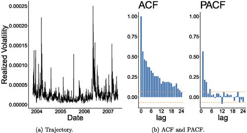
Fig. 6 One-step ahead prediction of the daily realized volatility of the FTSE 100 log-returns under the gamma-driven (left) and Poisson-driven (right) models with GIG marginals.

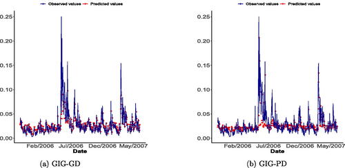
Table 1 Empirical means and RMSE (in parenthesis) of the maximum likelihood estimates for the GIG-GD process with $(\beta ,\delta ,\gamma )=(1,2,3)$, n = 500, 1000, 5000, and $\varphi =2,5$.

Parameters	n = 500	n = 1000	n = 5000
ϕ = 2	1.965 (0.333)	1.974 (0.233)	1.992 (0.102)
β = 1	0.931 (0.739)	0.993 (0.517)	0.998 (0.226)
δ = 2	2.109 (0.716)	2.032 (0.506)	2.014 (0.220)
γ = 3	2.975 (0.601)	3.013 (0.418)	2.993 (0.183)
ϕ = 5	4.957 (0.504)	4.995 (0.349)	5.003 (0.164)
β = 1	0.928 (0.834)	0.974 (0.569)	0.998 (0.257)
δ = 2	2.145 (0.859)	2.069 (0.569)	2.007 (0.257)
γ = 3	2.998 (0.659)	3.013 (0.466)	3.002 (0.205)

Table 2 Empirical means and RMSE (in parenthesis) of the maximum likelihood estimates for the Gamma-GD process with $(a,b)=(2,3)$, n = 500, 1000, 5000, and $\varphi =2,5$.

Parameters	n = 500	n = 1000	n = 5000
ϕ = 2	1.981 (0.250)	1.982 (0.173)	1.994 (0.079)
a = 2	2.032 (0.200)	2.015 (0.137)	2.002 (0.060)
b = 3	3.053 (0.271)	3.023 (0.192)	3.003 (0.081)
ϕ = 5	4.980 (0.440)	4.988 (0.306)	5.005 (0.138)
a = 2	2.060 (0.277)	2.027 (0.192)	2.002 (0.085)
b = 3	3.089 (0.356)	3.042 (0.249)	3.006 (0.108)

To get the standard errors of the maximum likelihood estimates, we propose using the Hessian matrix associated with the approximated log-likelihoods. To evaluate the performance of this approach, we perform Monte Carlo simulations where time series trajectories are generated from the GIG and gamma models, and confidence intervals are constructed for the parameters based on asymptotic normality and standard errors obtained via the Hessian matrix. If the standard errors are accurately estimated, the empirical coverages of the confidence intervals will be close from the nominal coverages. We consider 1000 Monte Carlo replications and parameter settings as before. Tables 3 and 4 provide the empirical coverages for the 90%, 95%, and 99% confidence intervals under the GIG and gamma cases, respectively. The empirical coverages are obtained as the proportion of times that the confidence intervals constructed in the Monte Carlo simulation contain the true value of the parameter. Looking at these tables, we can see that the proposed approach for getting standard errors and constructing confidence intervals for the parameters is working quite well since the empirical coverages are close to the desired ones for all cases considered. It is worth mentioning that in general Hessian matrix can be unstable and produce numerical issues, which cause problems to obtain standard errors based on it, but not in our case. Note that the complicated term of the log-likelihood function, the non-closed form integral, is replaced by a simple function via the Gauss-Laguerre expansion. This simplicity and the fact that such an approximation is accurate, explains why we did not experience issues with the Hessian matrix.

Table 3 Empirical coverages of confidence intervals for the parameters under the GIG-GD process with n = 500, 1000, 5000 when trajectories are generated from GIG-GD process.

Coverage →	90%	95%	99%	90%	95%	99%
$n\downarrow$	ϕ = 2			ϕ = 5
500	0.881	0.935	0.978	0.891	0.946	0.984
1000	0.895	0.943	0.977	0.916	0.952	0.992
5000	0.889	0.938	0.990	0.892	0.940	0.987
	β = 1			β = 1
500	0.889	0.945	0.984	0.902	0.943	0.988
1000	0.904	0.946	0.987	0.914	0.958	0.991
5000	0.905	0.954	0.992	0.916	0.951	0.991
	δ = 2			δ = 2
500	0.896	0.940	0.985	0.890	0.941	0.987
1000	0.906	0.949	0.987	0.910	0. 964	0.993
5000	0.905	0.954	0.988	0.910	0.956	0.990
	γ = 3			γ = 3
500	0.896	0.937	0.985	0.907	0.949	0.988
1000	0.892	0.954	0.986	0.907	0.950	0.990
5000	0.908	0.949	0.991	0.915	0.956	0.991

Table 4 Empirical coverages of confidence intervals for the parameters under the Gamma-GD process with n = 500, 1000, 5000 when trajectories are generated from Ga-GD process.

Coverage →	90%	95%	99%	90%	95%	99%
$n\downarrow$	ϕ = 2			ϕ = 5
500	0.888	0.934	0.982	0.898	0.938	0.985
1000	0.889	0.943	0.986	0.905	0.949	0.986
5000	0.874	0.939	0.988	0.900	0.953	0.991
	a = 2			a = 2
500	0.901	0.944	0.990	0.891	0.942	0.989
1000	0.908	0.960	0.993	0.901	0.958	0.993
5000	0.901	0.956	0.991	0.900	0.944	0.988
	b = 3			b = 3
500	0.896	0.948	0.986	0.898	0.941	0.987
1000	0.893	0.955	0.987	0.910	0. 964	0.993
5000	0.911	0.953	0.991	0.895	0.944	0.990

4 Generalizations

In this section we propose two generalizations of the gamma GD process to account for stylized features from realized volatility. We here consider a reparameterization of the gamma distribution in terms of mean and dispersion parameters for the marginals of the GD process addressed in this section. A random variable X following a gamma distribution with mean $\mu >0$ and dispersion $\kappa >0$ has density function given by $f(x)=\frac{{(\kappa /\mu )}^{\kappa }}{\Gamma (\kappa )}{x}^{\kappa -1}{e}^{-\kappa x/\mu }$, for x > 0. In this case, $E(X)=\mu$ and $\text{var}(X)={\mu }^2/\kappa$. This reparameterization can be obtained from $\Gamma (a,b)$ distribution by setting $a=\kappa$ and $b=\kappa /\mu$.

Remark 4.1.

Although we will be presenting such extensions for the gamma model, this can be easily be done for other distributions. For example, one could consider the inverse-Gaussian (IG) distribution (special case from the GIG model with $\beta =-1/2$) with parameterization in terms of the mean $\mu >0$ and variance ${\mu }^2/\kappa$, where κ is a dispersion parameter. The inclusion of covariates and long-memory extension for the IG model follow exactly as in the gamma case in what follows. An application of the IG long-memory model to a realized volatility data will be discussed in Section 5.2.

4.1 Inclusion of Covariates

We now define a nonstationary gamma GD process ${\left\{X_t\right\}}_{t\in \mathbb{N}}$ by assuming that its transition densities have the form (14) with κ and $\kappa /{\mu }_t$ replacing a and b, respectively, and ${\mu }_t=\hspace{0.17em}\mathrm{\text{exp}}\hspace{0.17em}({\psi }^{\top }{W}_t)$, where W_t is a matrix composed of $p\in \mathbb{N}$ time-varying covariates and ψ is a $p\times 1$ vector of associated regression coefficients to be estimated. Under this formulation, we have that $X_t\sim \Gamma (\kappa ,\kappa /{\mu }_t),E(X_t)={\mu }_t=\hspace{0.17em}\mathrm{\text{exp}}\hspace{0.17em}({\psi }^{\top }{W}_t)$, and $\text{var}(X_t)={\mu }_t^2/\kappa$, for $t\in \mathbb{N}$. Therefore, the model allows for nonstationary positive time series and covariates can be included in the model through the mean as in generalized linear models. Let us denote this model by Ga-GLMGD.

The maximum likelihood estimation (MLE) of parameters is performed similarly as in the stationary case discussed previously, with the log-likelihood function assuming a similar form as (18) with a and b replaced by κ and $\kappa /{\mu }_t$ (note that one of the parameters now is time-varying), respectively. The parameter vector here is $(\varphi ,\kappa ,{\psi }^{\top })$ and we estimate it via maximum likelihood.

We now present a small Monte Carlo simulation to check the performance of the MLEs. We generate a covariate time series W_t through a logit transformation of a realization of a first-order autoregressive process, say Z_t (with autoregressive coefficient 0.5 and variance noise equal to 1), that is $W_t=\text{logit}(Z_t)=\frac{e^{Z_t}}{1+e^{Z_t}}$, for $t=1,\dots ,n$. The idea here is to mimic a bounded time series covariate on the interval (0, 1) that is important to explain the response time series. The following settings are assumed for this Monte Carlo simulation (with 1000 replications): n = 500, 1000, ϕ = 5, κ = 3, ${\psi }_0=0.1$ (intercept) and ${\psi }_1=-0.2$. Table 5 provides the empirical means and RMSE of the maximum likelihood estimates obtained in the Monte Carlo simulation. We can notice that the estimation of the parameters via MLE is working well.

Table 5 Empirical means and RMSE (in parentheses) of the maximum likelihood estimates for the Ga-GLMGD process with ϕ = 5, κ = 3, ${\psi }_0=0.1,{\psi }_1=-0.2$, and sample sizes n = 500, 1000.

Parameter	n = 500	n = 1000
ϕ = 5	4.982 (0.494)	4.971 (0.341)
κ = 3	3.067 (0.333)	3.031 (0.235)
${\psi }_0=0.1$	0.081 (0.118)	0.084 (0.082)
${\psi }_1=-0.2$	–0.161 (0.206)	–0.168 (0.143)

4.2 Long-Memory Modeling

Inspired by the work by Corsi (2009), we now extend the GD processes to handle long-memory time series, which is an important feature to be considered when modelling realized volatility for many years. Let ${\left\{X_t\right\}}_{t\in \mathbb{N}}$ be a stochastic process and denote ${\mathcal{F}}_{t-1}=\sigma (X_{t-1},X_{t-2},\dots ,X_1)$, that is, the σ-algebra generated by $X_{t-1},X_{t-2},\dots ,X_1$. We define a gamma long-memory GD process by assuming that its transition densities have the form (14) with κ and $\kappa /{\mu }_t$ replacing a and b, respectively, and ${\mu }_t\equiv E(X_t|{\mathcal{F}}_{t-1})$ given by (21) $${\mu }_t={\psi }_0+{\psi }_1{X}_{t-1}+{\psi }_2\frac{1}{4}\sum _{i=1}^4{X}_{t-i-1}+{\psi }_3\frac{1}{17}\sum _{i=5}^{21}{X}_{t-i-1},$$(21) where ${\psi }_0>0$, and ${\psi }_1,{\psi }_2,{\psi }_3\ge 0$ are parameters to be estimated, $\frac{1}{4}{\sum }_{i=1}^4{X}_{t-i-1}$ is a medium-term investors who rebalance weekly and $\frac{1}{17}{\sum }_{i=5}^{21}{X}_{t-i-1}$ is a long-term investors who rebalance their positions after one or more months; for instance, see Pascalau and Poirier (2023). Note that the short-term traders with a daily, or shorter rebalance frequency, in other words, the dependence on $X_{t-1}$ enters the model via the conditional expectation μ_t (see Equation (21)(21) $${\mu }_t={\psi }_0+{\psi }_1{X}_{t-1}+{\psi }_2\frac{1}{4}\sum _{i=1}^4{X}_{t-i-1}+{\psi }_3\frac{1}{17}\sum _{i=5}^{21}{X}_{t-i-1},$$(21) ) and also through the latent gamma process ${\left\{Y_t\right\}}_{t\in \mathbb{N}}$ introduced in Section 2.

Remark 4.2.

It is worth mentioning that the nomenclature long-memory GD processes refers to the ability of such models to provide a good approximation for handling positive continuous long-memory time series and not to its theoretical property since in theory these models are short-memory like Corsi’s (2009) model.

As in the model introduced in Section 4.1, the log-likelihood function for the long-memory GD process has the form (18) with a and b replaced by κ and $\kappa /{\mu }_t$, with μ_t given by (21). The standard maximum likelihood method can be applied to obtain parameter estimates and to perform inference as well. The gamma long-memory GD model (in short Ga-LMGD) will be applied to a realized volatility data in Section 5.2.

5 Realized Volatility Data Analysis

In this section, we apply the gamma-driven models to the daily realized volatility of FTSE 100 equity index log-returns computed every 10 min from October 31st, 2003, to May 31st, 2007. We will initially analyze this realized volatility for this “short” period of time but in Section 5.2 a longer period will be considered, which requires a more complex modeling where long-memory can be accommodated. These data can be found at Heber et al. (2020) and consist of 939 observations. There are 38 missing observations (corresponding to holidays and weekends) and one outlier (corresponding to an isolated fact that occurred in London). The missing observations were not considered, and the outlier was replaced by a missing value (NA) and then imputed using the R package mice. These data have also been considered and analyzed by Anzarut et al. (2018), where a similar treatment for missing values and imputation was considered. After the data cleaning, we end up with 901 observations. For other recent works dealing with realized volatility, for instance, see Chen et al. (2018), Chen, Watanabe, and Lin (2021), and Takahashi, Watanabe, and Omori (in press).

Table 6 presents some descriptive statistics for the daily realized volatilities. Figure 5 shows the realized volatility and its associated ACF and PACF plots. These plots indicate a stationary behavior of the time series data.

Table 6 Descriptive statistics for the daily realized volatility of the FTSE 100 equity index log-returns computed every 10 min from October 31st, 2003, to May 31st, 2007.

n	Minimum	Maximum	Mean	Median	Standard deviation
901	$3.091\times {10}^{-6}$	$2.501\times {10}^{-4}$	$2.58\times {10}^{-5}$	$2.003\times {10}^{-5}$	$2.397\times {10}^{-5}$

We fit the GD processes to the realized volatilities multiplied by 1000. Then, we consider the maximum likelihood approach combined with the Gauss Laguerre quadrature to estimate the parameters under the GIG and gamma GD models. The maximum likelihood estimates, standard errors, and 95% confidence intervals for the parameters under the GIG and gamma assumptions are provided in Tables 7 and 8, respectively.

Table 7 Maximum likelihood estimates, standard errors, and 95% confidence intervals for the parameters under the GIG-GD process.

Parameters	Estimates	stand. err.	95% CI
ϕ	4.082	0.293	(3.507, 4.67)
$\beta$	–2.007	0.366	(–2.725, –1.289)
$\delta$	0.074	0.008	(0.058, 0.091)
$\gamma$	17.677	10.827	(0.000,38.897)

Table 8 Maximum likelihood estimates, standard errors, and 95% confidence intervals for the parameters under the Gamma-GD process.

Parameters	Estimates	stand. err.	95% CI
ϕ	4.929	0.308	(4.325, 5.532)
a	1.424	0.177	(1.078, 1.771)
b	55.134	5.653	(44.053, 66.214)

We check if the GIG and gamma GD models are fitting well the daily realized volatility considered here. To do that, we consider residual analyses with simulated envelopes and a probability integral transform approach. To save space in the article, all the results are presented in Section 3 of the supplementary materials. In summary, the goodness-of-fit analyses showed that both models are well-fitted to the data.

In what follows, we investigate whether the GIG and gamma GD models provide a suitable fit to the realized volatility and perform an out-of-sample prediction exercise. A comparison with a discrete-time Poisson-driven model by Anzarut et al. (2018) will also be presented.

5.1 Out-of-Sample Prediction

To assess the performance of the models in terms of forecasting, an out-of-sample prediction exercise is considered as done, for instance, in Agosto et al. (2016). This method divides the sample of size T into two parts. The first with size $T_0,\{x_{t-1}:t=1,\dots ,T_0\}$ is used to for the initial model estimation, and the remaining observations, of size $T-T_0,\{x_{t-1}:t=T_0+1,\dots ,T\}$, are used to the forecasting exercise. Given the parameter estimate using just the information until the time t, the corresponding one-step ahead forecast of $x_{t+1}$ is calculated as ${\widehat{x}}_{t+1|t}=\widehat{E}(X_{t+1}|X_t)$. This exercise is repeated for $t=T_0+1,\dots ,T$, thus, providing a sequence of one-step ahead predictions $\{{\widehat{x}}_{t+1|t}:t=T_0,\dots ,T\}$. To evaluate the predictive power of the models, we consider the mean square forecasting error (MSFE) $${\text{MSFE}}_t=\frac{1}{t-T_0}\sum _{s=T_0}^T{(x_{s+1}-{\widehat{x}}_{s+1|s})}^2,\hspace{1em}t=T_0+1,\dots ,T,$$

and the forecasting score (FS) $$\begin{array}{c}{\text{FS}}_t=\frac{1}{t-T_0}\sum _{s=T_0}^T(x_{s+1}\hspace{0.17em}\mathrm{\text{log}}\hspace{0.17em}({\widehat{x}}_{s+1|s})-{\widehat{x}}_{s+1|s}),\\ \mathrm{\hspace{1em}}\mathrm{\hspace{1em}}t=T_0+1,\dots ,T.\end{array}$$

For sake of comparison, we also consider here the discrete-time Poisson-driven model with GIG marginals (GIG-PD) by Anzarut et al. (2018). We performed maximum likelihood estimation of parameters and a summary is provided in Table 9 (using all the data); the parameter ϕ here is related to the latent Poisson variable from Anzarut et al.’s (2018) model.

Table 9 Maximum likelihood estimates, standard errors, and 95% confidence intervals for the parameters under the GIG-PG process.

Parameters	Estimates	stand. err.	95% CI
ϕ	96.43623	8.976	(81.672, 111.200)
β	–2.509	0.505	(–3.341, –1.678)
δ	0.289	0.016	(0.262, 0.316)
γ	0.388	25.530	(0.000, 42.382)

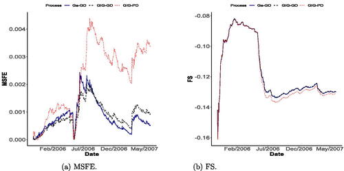
The prediction exercise was performed to the realized volatility with $T_0=500$, and initial 401 observations were used for the initial estimation of the model. Figure 6 shows the observed times series and one-ahead forecasts according to GIG-GD and GIG-PD models. We do not present the plot for the GD-Ga model to save space in the article since it was quite similar to the GIG-GD one. This plot reveals that our method is providing better predictions than the GIG-PD approach. This can be also be noticed from Figure 7, which provides the MSFE and FS plots for the fitted Ga-GD, GIG-GD, and GIG-PD processes. The smallest MSFEs are produced by the gamma-driven models, which are performing better than the Poisson-driven model. Regarding the FS (the higher, the better the model), Ga-GD and GIG-GD model performances are almost indistinguishable and still provide better results than the GIG-PD model.

Fig. 7 MSFE (on the left) and FS (to the left) plots for the fitted Ga-GD, GIG-GD, and GIG-PD processes.

5.2 Long-Memory Analysis

We now consider the realized volatility of FTSE 100 for a longer period, from January 2nd, 2004 to December 4th, 2017. In this case, the gamma driven and Poisson-driven Markov processes are not suitable for analyzing this data and a more complex model is necessary. As pointed out by one of the Referees, even for a shorter period of time, these models might not enough capture key features and this is reflected by some large standard errors of estimates; for instance, see Tables 7 and 9. That is our motivation for proposing the long-memory extension of our GD processes in Section 4.2 inspired by the work by Corsi (2009), as suggested by the AE. After cleaning the data (following the same procedures as at the beginning of the section), we end up with n = 3508 observations, which are multiplied by 1000 (as before). Table 10 provides a descriptive analysis, while Figure 8 shows plots of the realized volatility of FTSE 100 and its associated ACF and PACF.

Fig. 8 Plots of the realized volatility of FTSE 100 (multiplied by 1000) from January 2, 2004 to December 4, 2017 and its associated ACF and PACF.

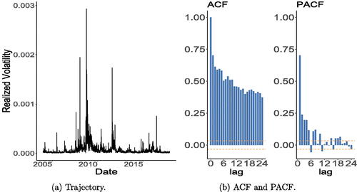
Table 10 Descriptive statistics for the daily realized volatility of the FTSE 100 equity index log-returns computed every 10 min from January 2nd, 2004 to December 4th, 2017.

n	Minimum	Maximum	Mean	Median	Standard deviation
3508	$2.947\times {10}^{-6}$	$2.931\times {10}^{-3}$	$6.718\times {10}^{-5}$	$3.236\times {10}^{-5}$	$1.273\times {10}^{-4}$

The summary fits of Ga-LMGD and IG-LMGD are respectively presented in Tables 11 and 12, respectively. From these tables, we can observe relatively small standard errors and parameter estimates “far from zero,” which is an indication that the components included in the model are significant. In particular, an interesting fact is that the nonlinear incorporation of $X_{t-1}$ to explain X_t seems to be significant under both gamma and IG models. Of course, the null hypothesis $H_0:\varphi =0$ belongs to the boundary of the parameter space and this should be tested adequately; a likelihood ratio test can be used and the asymptotic distribution is not longer Chi-squared distributed, but a 50%–50% mixture between a Chi-square distribution and a degenerated distribution at 0. Anyway, the estimate of ϕ is not close to zero and the standard error is small, which gives us evidence that this nonlinearity is important to be considered through our proposed gamma-driven approach. Also, note that $X_{t-1},\frac{1}{4}{\sum }_{i=1}^4{X}_{t-i-1}$ and $\frac{1}{17}{\sum }_{i=5}^{21}{X}_{t-i-1}$ also seem to be significant to be included in the gamma LMGD process to explain the conditional mean (in a linear way). On the other hand, $X_{t-1}$ seems to be not significant to explain the conditional mean (in a linear way) under the inverse-Gaussian LMGD model. These results show the importance of considering a nonlinear relationship between X_t and $X_{t-1}$ in the analysis of realized volatility, which is a relevant finding of this article.

Table 11 Maximum likelihood estimates, standard errors, and 95% confidence intervals for the parameters under the gamma long-memory GD process.

Parameter	Estimates	stand. err.	95% CI
ϕ	1.247	0.123	(1.044, 1.449)
κ	3.048	0.098	(2.887, 3.209)
ψ0	0.004	0.001	(0.003, 0.005)
ψ1	0.269	0.029	(0.222,0.316)
ψ2	0.499	0.040	(0.433, 0.565)
ψ3	0.131	0.027	(0.087, 0.175)

Table 12 Maximum likelihood estimates, standard errors, and 95% confidence intervals for the parameters under the inverse-Gaussian long-memory GD process.

Parameter	Estimates	stand. err.	95% CI
ϕ	2.808	0.150	(2.561, 3.056)
κ	0.074	0.003	(0.070, 0.079)
ψ0	0.009	0.001	(0.008, 0.011)
ψ1	0.008	0.019	(0.000, 0.040)
ψ2	0.540	0.057	(0.446, 0.633)
ψ3	0.169	0.047	(0.092, 0.246)

To conclude the realized volatility analysis, we evaluate the forecast power of our long-memory models by performing an out-of-sample prediction exercise as described in Section 5.1 with $T_0=2000$. For sake of comparison, we consider the performance of the GIG and gamma GD processes. We additionally include Corsi’s model that serves as an interesting benchmark, where we have used least squares method to estimate its parameters.

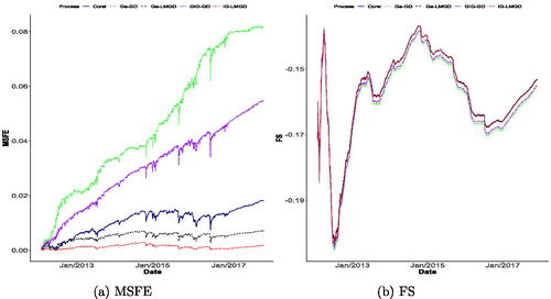
The MSFE and FS plots are displayed in Figure 9, which reveals the superior performance of the long-memory models over the Markovian ones, as expected, especially in terms of MSFE. Among those models that can capture long-memory, we notice that our long-memory processes perform better than Corsi’s model, which is already expected since they are designed to handle continuous positive time series, while Corsi’s model is $\mathbb{R}$-valued. It is worth mentioning again that these models are in theory short-memory, but they are capable of handling long-memory time series well, as discussed in Remark 4.2.

Fig. 9 MSFE (on the left) and FS (to the left) plots based on Ga-LMGD, IG-LMGD, Corsi, Ga-GD, and GIG-GD models.

6 Concluding Remarks

We proposed a novel method to construct a Markovian model with desirable ${\mathbb{R}}_{+}$ marginals based on a gamma latent variable. Properties of our gamma-driven (GD) models were explored, in particular, its time-reversibility, and explicit form for the transition densities. The likelihood function of GD models depend on integrals without closed form, which makes inference more challenging. To overcome this issue, we approximated such integrals via Gauss Laguerre quadrature. Then, we proposed estimation of parameters through maximum likelihood using the approximated likelihood function. Extensive simulated results gave us evidence that the proposed estimation procedure produces accurate estimates and reliable standard errors obtained via the resulting approximated Hessian matrix. Two generalizations of GD processes for dealing with nonstationary and long-memory time series were proposed. Applications of our methodologies to the daily realized volatility of FTSE 100 equity index log-returns were presented and compared to the discrete-time Poisson-driven (PD) models by Anzarut et al. (2018). These empirical applications showed that GD processes and their generalizations can be produce better results in terms of prediction over PD models. Table 13 provides the computational time (in seconds) to fit a GD process or one of its generalizations for the simulated (one replica) or real datasets (n denotes the sample size) considered in this article, which gives an idea about the scalability of our approches. As can be seen, the models requiring more computational efforts are the gamma and inverse-Gaussian long-memory GD processes for the realized volatility data analysis consisting of n = 3508 observations. Anyway, less than 1 min is needed to fit such a data under both models.

Table 13 Computational time in seconds to fit GD processes and their generalizations for simulated and real data considered in this article; n here denotes the sample size.

Model	Computational time
Simulated data, Section 3, GIG-GD (n = 500)	1.247
Simulated data, Section 3, GIG-GD (n = 1000)	4.048
Simulated data, Section 3, GIG-GD (n = 5000)	9.252
Simulated data, Section 3, Ga-GD (n = 500)	0.495
Simulated data, Section 3, Ga-GD (n = 1000)	0.925
Simulated data, Section 3, Ga-GD (n = 5000)	3.841
Simulated data, Section 4.1, Ga-GLMGD (n = 500)	1.936
Simulated data, Section 4.1, Ga-GLMGD (n = 1000)	3.665
Data analysis, Section 5, GIG-GD (n = 901)	5.245
Data analysis, Section 5, Ga-GD (n = 901)	1.888
Data analysis, Section 5.2, Ga-GLMGD (n = 3508)	59.572
Data analysis, Section 5.2, IG-GLMGD (n = 3508)	36.02

We believe that there are many points deserving further investigation. The generalizations we proposed for GD processes allowing for inclusion of covariates and to handle long-memory time series can also be adapted to extend the Poisson-driven models by Anzarut et al. (2018). One of the Referees suggested us to extend our GD approach to the continuous time as done by Anzarut et al. (2018). In order to obtain such an extension we need to prove that the transition densities of GD Markov process satisfy the Chapman-Kolmogorov equations. Under our approach, such an extension seems to be complicated since it involves a functional equation that we are not able to solve. Whereas, in the case of the Poisson-driven model by Anzarut et al. (2018), it arises the well-known Cauchy’s exponential functional equation. Another point to be investigated in future research are the long-memory GD models introduced in Section 4.2. The application of such models to realized volatility, say $\left\{X_t\right\}$, indicates that is important to include $X_{t-1}$ in both nonlinear and linear ways in the models to explain X_t. A formal hypotheses testing in this case is more challenge since the null hypothesis belongs to the boundary of the parameter space. We believe that the restricted bootstrap by Cavaliere, Nielsen, and Rahbek (2016) is a great tool to cope this problem and we hope to report results on that soon in a future paper. Finally, other extensions of the GD processes by incorporating stylized features such as unobserved components and jumps with stochastic (possibly self-exciting) intensity (for instance, see Li and Zinna (2018)) are worth investigation.

Supplementary Materials

The supplementary material contains additional numerical results from simulated and real data and an evaluation of the Gaussian Laguerre quadrature for a simple example.

Acknowledgments

We thank the Editor Prof. Atsushi Inoue, AE and two anonymous Referees for their constructive criticisms that led the article to a substantial improvement.

Disclosure Statement

The authors report there are no competing interests to declare.

Additional information

Funding

F.G.B. Mendes acknowledges the financial support from Coordenação de Aperfeiçoamento de Pessoal de Nível Superior (CAPES-Brazil).

References

- Abramowitz, M., and Stegun, I. A. (1974), Handbook of Mathematical Functions, With Formulas, Graphs, and Mathematical Tables, New York: Dover Publications, Inc.
- Agosto, A., Cavaliere, G., Kristensen, D., and Rahbek, A. (2016), “Modeling Corporate Defaults: Poisson Autoregressions with Exogenous Covariates (PARX),” Journal of Empirical Finance, 38, 640–663. DOI: 10.1016/j.jempfin.2016.02.007.
- Al-Osh, M. A., and Alzaid, A. A. (1987), “First-Order Integer-Valued Autoregressive (INAR(1)) Process,” Journal of Time Series Analysis, 8, 261–275. DOI: 10.1111/j.1467-9892.1987.tb00438.x.
- Anzarut, M., Mena, R. H., Nava, C. R., and Prünster, I. (2018), “Poisson-Driven Stationary Markov Models,” Journal of Business and Economic Statistics, 36, 684–694. DOI: 10.1080/07350015.2016.1251441.
- Cavaliere, G., Nielsen, H., and Rahbek, A. (2016), “On the Consistency of Bootstrap Testing for a Parameter on the Boundary of the Parameter Space,” Journal of Time Series Analysis, 38, 513–534. DOI: 10.1111/jtsa.12214.
- Corsi, F. (2009), “A Simple Approximate Long-Memory Model of Realized Volatility,” Journal of Financial Econometrics, 7, 174–196. DOI: 10.1093/jjfinec/nbp001.
- Chen, X. B., Gao, J. H., Li, D., and Silvapulle, P. (2018), “Nonparametric Estimation and Forecasting for Time-Varying Coefficient Realized Volatility Models,” Journal of Business and Economic Statistics, 36, 88–100. DOI: 10.1080/07350015.2016.1138118.
- Chen, X. B., Watanabe, T., and Lin, E. (2023), “Bayesian Estimation of Realized GARCH-Type Models with Application to Financial Tail Risk Management,” Econometrics and Statistics, 28, 30–46. DOI: 10.1016/j.ecosta.2021.03.006.
- Contreras-Cristán, A., Mena, R. H., and Walker, S. G. (2009), “On the Construction of Stationary AR(1) Models via Random Distributions,” Statistics, 43, 227–240. DOI: 10.1080/02331880802259391.
- Gaver, D. P., and Lewis, P. A. W. (1980), “First-Order Autoregressive Gamma Sequences and Point Processes,” Advances in Applied Probability, 12, 727–745. DOI: 10.2307/1426429.
- Heber, G., Shephard, N., Sheppard, K., Lunde, A., Sharp, J., Hendricks, D., and Pesch, D. (2020), “Oxford-Man Institute’s Realized Library, version 0.3,” https://realized.oxford-man.ox.ac.uk/data.
- Jacobs, P. A., and Lewis, P. A. W. (1977), “A Mixed Autoregressive-Moving Average Exponential Sequence and Point Process (EARMA 1,1),” Advances in Applied Probability, 9, 87–104. DOI: 10.2307/1425818.
- Jacobs, P. A., and Lewis, P. A. W. (1978), “Discrete Time Series Generated by Mixtures II: Asymptotic Properties,” Journal of the Royal Statistical Society, Series B, 40, 222–228. DOI: 10.1111/j.2517-6161.1978.tb01667.x.
- Joe, H. (1980), “Time Series Models with Univariate Margins in the Convolution-Closed Infinitely Divisible Class,” Journal of Applied Probability, 33, 664–677. DOI: 10.2307/3215348.
- Kahaner, D., Moler, C., and Nash, S. (1989), Numerical Methods and Software, Upper Saddle River, NJ: Prentice Hall.
- Lawrance, A. J., and Lewis, P. A. W. (1977), “An Exponential Moving-Average Sequence and Point Process (EMA1),” Journal of Applied Probability, 14, 98–113. DOI: 10.2307/3213263.
- Leisen, F., Mena, R., Palma, F., and Rossini, L. (2019), “On a Flexible Construction of a Negative Binomial Model, Statistics and Probability Letters, 152, 1–8. DOI: 10.1016/j.spl.2019.04.004.
- Li, J., and Zinna, G. (2018), “The Variance Risk Premium: Components, Term Structures and Stock Return Predictability,” Journal of Business and Economic Statistics, 36, 411–425. DOI: 10.1080/07350015.2016.1191502.
- McKenzie, E. (1985), “Some Simple Models For Discrete Variate Time Series,” Journal of the American Water Resources Association, 21, 645–650. DOI: 10.1111/j.1752-1688.1985.tb05379.x.
- Mena, R. H., and Walker, S. G. (2005), “Stationary Autoregressive Models via a Bayesian Nonparametric Approach,” Journal of Time Series Analysis, 26, 789–805. DOI: 10.1111/j.1467-9892.2005.00429.x.
- Palma, F. & Mena, R.H. (2021). Duality for a class of continuous-time reversible Markov models, Statistics 55, 231–242. DOI: 10.1080/02331888.2021.1881098.
- Pascalau, R., and Poirier, R. (2023), “Increasing the Information Content of Realized Volatility Forecasts, Journal of Financial Econometrics, 21, 1064–1098. DOI: 10.1093/jjfinec/nbab028.
- Pitt, M. K., Chatfield, C., and Walker, S. G. (2002), “Constructing First Order Stationary Autoregressive Models via Latent Processes,” Scandinavian Journal of Statistics, 29, 657–663. DOI: 10.1111/1467-9469.00311.
- Takahashi, M., Watanabe, T., and Omori, Y. (in press), “Forecasting Daily Volatility of Stock Price Index Using Daily Returns and Realized Volatility,” Econometrics and Statistics. DOI: 10.1016/j.ecosta.2021.08.002.