Gaussian Process Vector Autoregressions and Macroeconomic Uncertainty

Abstract

We develop a nonparametric multivariate time series model that remains agnostic on the precise relationship between a (possibly) large set of macroeconomic time series and their lagged values. The main building block of our model is a Gaussian process prior on the functional relationship that determines the conditional mean of the model, hence, the name of Gaussian process vector autoregression (GP-VAR). A flexible stochastic volatility specification is used to provide additional flexibility and control for heteroscedasticity. Markov chain Monte Carlo (MCMC) estimation is carried out through an efficient and scalable algorithm which can handle large models. The GP-VAR is used to analyze the effects of macroeconomic uncertainty, with a particular emphasis on time variation and asymmetries in the transmission mechanisms.

KEYWORDS:

• Asymmetric uncertainty shocks
• Bayesian nonparametrics
• Nonlinear vector autoregressions

1 Introduction

Economic relations can change over time for a variety of reasons, such as technological progress, institutional changes, major policy interventions, but also wars, terrorist attacks, stock market crashes and pandemics. Standard econometric models, such as linear single and multivariate regressions assume instead stability of the parameters characterizing the conditional first and second moments of the dependent variables. When stability is formally tested, it is often rejected (see, e.g., Stock and Watson 1996). This has led to the development of a variety of methods to handle structural change in econometric models.

Parameter evolution is assumed to be either observable (i.e., driven by the behavior of observable economic variables) or unobservable, and either discrete and abrupt or continuous and smooth. Examples include threshold and smooth transition models (see, e.g., Tong 1990; Teräsvirta 1994), Markov switching models (see, e.g., Hamilton 1989), and double stochastic models (see, e.g., Nyblom 1989). Examples of economic applications of these methods include Koop and Korobilis (2013), Aastveit, et al. (2017), Caggiano, Castelnuovo, and Pellegrino (2017), Alessandri and Mumtaz (2019), Caggiano, Castelnuovo, and Pellegrino (2021), and Barnichon, Debortoli, and Matthes (2022).¹ Another recent strand of the literature, pioneered in Barnichon and Matthes (2018), approximates impulse responses through a number of Gaussian basis functions. These models are fully parametric and therefore specify the type of parameter nonlinearities a priori.

Assuming a specific type of parameter evolution increases estimation efficiency but can lead to mis-specification. A more flexible alternative allows for a smooth evolution of parameters without specifying the form of parameter time variation. In a classical context, the evolution can be either deterministic (see, e.g., Robinson 1991; Chen and Hong 2012), or stochastic (see, e.g., Giraitis, Kapetanios, and Yates,2014 2018; Kapetanios, Marcellino, and Venditti,2019 for the specific case of (possibly large) vector autoregressive models (VARs)). Kernel estimators are the main tool used in this literature. Alternative approaches are, for example, based on using functional-coefficient regressions (Cai, Fan, and Yao 2000; Kowal, Matteson, and Ruppert 2017), Gaussian random fields (Hamilton 2001), regression trees (Chipman, George, and McCulloch 2010; Huber et al.2023), neural networks (Hornik, Stinchcombe, and White 1989; Gu, Kelly, and Xiu 2021; Coulombe 2022) or Bayesian nonparametrics (BNP) based on infinite mixtures (Hirano 2002; Bassetti, Casarin, and Leisen 2014; Kalli and Griffin 2018; Bassetti, Casarin, and Rossini 2020; Jin, Maheu, and Yang 2022). These popular machine learning methods, however, are difficult to interpret and need substantial tuning to work well on comparatively short macroeconomic time series such as the ones considered in this article. Moreover, some of these techniques do not scale well into high dimensions and are thus not particularly suited for large panels nowadays used in macroeconomics.

In this article, we propose a new model that belongs to the nonparametric class and is capable of capturing, in a flexible way, general nonlinear relationships. We combine the statistical literature on Gaussian process (GP) regressions (see, e.g., Crawford et al.2019), with that on VARs to obtain a GP-VAR model. Borrowing ideas from the literature on Bayesian Minnesota-type VARs, we assume, for each endogenous variable, a different nonlinear relationship with its own lags and with the lags of all the other variables (and possibly of additional exogenous regressors). Gaussian processes are used to model nonlinearities in a flexible but efficient way and are related to popular techniques such as neural networks.² Another related approach is the BNP-VAR of Billio, Casarin, and Rossini (2019). Similarly to the GP-VAR the object of interest is the posterior distribution over a functional space which requires the specification of a suitable prior process. Our model assumes that the shocks are Gaussian. To add flexibility we introduce a novel stochastic volatility (SV) specification to allow for smoothly varying error variances. The use of SV in the GP-VAR adds flexibility, and prevents overfitting as it avoids that large realizations of the shocks are interpreted as changes in the conditional mean.

We develop an efficient Bayesian estimation procedure, based on the structural form of the GP-VAR, which has the additional benefit that its complexity is linear in the number of endogenous variables and does not depend on the number of lags. Hence, estimation can be parallelized and, in addition, introducing conditionally conjugate priors allows for pre-computing various matrix multiplications and kernel operations, which further speeds up computation. As a result, estimation is feasible also for very large models.

Our GP-based model has a vast range of applicability, for both reduced form and structural analysis. This mirrors the possible applications of standard VARs but allows for more general dynamic relationships across the variables. As an example of a structural economic analysis, and to gather new insights on a topic that has recently attracted considerable attention (see, e.g., Bloom 2014), we use the GP-VAR to investigate the effects of uncertainty shocks on U.S. macroeconomic and financial indicators. First, we show that applying our approach to data simulated from the structural model by Basu and Bundick (2017) delivers impulse response functions closer to the true ones than a linear BVAR. Then, by using real data, we compare the responses of the GP-VAR with those of a standard linear BVAR. Differences relate to the shape and magnitudes, with the GP-VAR producing stronger reactions for selected macro quantities.

Our proposed framework naturally allows for analyzing potential asymmetries in transmission channels. The responses to a positive uncertainty shock (higher unexpected uncertainty) are typically much stronger than those to a negative shock. Interestingly, the shape of the IRFs also differ, with positive shocks leading to responses that peak later. In addition, our findings suggest that the relationship between real activity and uncertainty becomes proportionally slightly smaller for large shocks, while financial markets react relatively more strongly to larger increases in uncertainty. Our framework also permits to investigate whether transmission mechanisms have changed over time. Doing so indicates that the effects of uncertainty have been increasing up to 2007Q1 before turning more muted afterwards. Finally, we find that asymmetry moves with variables closely related to the business cycle.

The article is structured as follows. Section 2 provides an introduction to Gaussian process regression. Section 3 develops the GP-VAR model. It also provides details on the prior setup and posterior computation. Section 4 deals with the macroecononomic effects of uncertainty shocks through the lens of our flexible nonparametric model. The final section briefly summarizes and concludes the article. The Online Appendix contains technical details on the specification, estimation and use of the GP-VAR model and additional empirical results such as simulation findings, forecasting results using U.S. data and in-sample model features.

2 A Brief Introduction to Gaussian Processes

In this section we briefly discuss Gaussian process (GP) regressions, focusing on time series data.³ GP regressions are a nonparametric technique to establish a flexible relationship between a scalar time series y_t and a set of K predictors ${\mathit{x}}_t$ in period $t=1,\dots ,T$ where T marks the end of the sample. Their key advantage is that they do not rely on parametric assumptions on the precise functional relationship between y_t and ${\mathit{x}}_t$.

In general, a nonparametric regression is given by $$y_t=f({\mathit{x}}_t)+{\epsilon }_t,\hspace{1em}{\epsilon }_t\sim \mathcal{N}(0,{\sigma }^2),$$with f being some unknown regression function $f:{\mathbb{R}}^K\to \mathbb{R}$ and ${\epsilon }_t$ denoting an independent Gaussian shock with zero mean and constant variance ${\sigma }^2$. We relax this assumption in Section 3.1 to allow for heteroscedastic shocks. An assumption on the error distribution is needed in a Bayesian context and Gaussianity is the most common one, though different distributions can be easily accommodated by exploiting a scale-location mixture of Gaussians representation (see, e.g., Escobar and West 1995).

In standard regression models, the function f is assumed to be linear with $f({\mathit{x}}_t)=\mathit{\beta }\prime {\mathit{x}}_t$ where $\mathit{\beta }$ is a $K\times 1$ vector of linear coefficients. If mean relations are nonlinear, this assumption might be too restrictive. To gain more flexibility one can embed the covariates in ${\mathit{x}}_t$ into a higher dimensional space such as the space of powers ${\mathit{x}}_t\to \psi ({\mathit{x}}_t)=(\mathit{x}{\prime }_t,({\mathit{x}}_t^2)\prime ,\dots ,({\mathit{x}}_t^R)\prime )\prime$, with ${\mathit{x}}_t^2=({\mathit{x}}_t\odot {\mathit{x}}_t)$ and higher orders defined recursively. Conditional on choosing a sufficiently large integer R, this would provide substantial flexibility to approximate any smooth function f. However, adequately selecting R is key and the mapping, moreover, is ad-hoc in the sense that there exist infinitely many nonlinear mappings ψ.

Standard Bayesian methods place a prior on the coefficients associated with the covariates (and possible nonlinear transformations thereof) and thus control for uncertainty with respect to these basis functions but at the cost of remaining within a class of functions (such as linear, polynomial or trigonometric). By contrast, GP regressions treat the function f as an unknown quantity and let the data decide about the appropriate form (and degree) of nonlinearity.

2.1 Estimating Unknown Functions: The Function Space View

The key inferential goal in GP regression is to infer the function f from the data under relatively mild assumptions. This is achieved by specifying a prior on $f({\mathit{x}}_t)$. A typical assumption is to assume that $f({\mathit{x}}_t)$ follows a Gaussian process prior: $$f({\mathit{x}}_t)\sim \mathit{\text{GP}}\left(\mu ({\mathit{x}}_t),k_{\mathit{\vartheta }}({\mathit{x}}_t,{\mathit{x}}_t)\right),$$

with $\mu ({\mathit{x}}_t)=\mathbb{E}[f({\mathit{x}}_t)]$ being the mean function and $$k_{\mathit{\vartheta }}({\mathit{x}}_t,{\mathit{x}}_{\tau })=\mathbb{E}[(f({\mathit{x}}_t)-\mu ({\mathit{x}}_t))(f({\mathit{x}}_{\tau })-\mu ({\mathit{x}}_{\tau }))]$$denoting a kernel (or covariance) function that relates $f({\mathit{x}}_t)$ and $f({\mathit{x}}_{\tau })$ for periods t and τ. The kernel is typically parameterized by a low dimensional vector of hyperparameters $\mathit{\vartheta }$ and controls the behavior of the function f. This kernel needs to be positive semidefinite and symmetric.

We set the function $\mu ({\mathit{x}}_t)=0$ for all t, without loss of generality, since any explicit basis function for $\mu ({\mathit{x}}_t)$ can be used to model the mean process. If the focus is on modeling stationary data, $\mu ({\mathit{x}}_t)=0$ implies that a priori the process is centered around a white-noise process. If one would like to model persistent or nonstationary data, it would be straightforward to implement a prior that forces the system toward a set of random walk processes.⁴ A common choice in GP regressions is the Gaussian (or squared exponential) kernel function: $$k_{\mathit{\vartheta }}({\mathit{x}}_t,{\mathit{x}}_{\tau })=\xi \times \hspace{0.17em}\mathrm{\text{exp}}\hspace{0.17em}\left(-\frac{\kappa }{2}{\Vert {\mathit{x}}_t-{\mathit{x}}_{\tau }\Vert }^2\right),$$with ξ denoting a scaling parameter and κ the (inverse) length scale and thus $\mathit{\vartheta }=(\xi ,\kappa )\prime$. Larger values of κ lead to a GP which displays more high frequency variation whereas lower values imply a slowly varying mean function. The parameter ξ controls the prior variance of the function f. To see this, note that if ${\mathit{x}}_t={\mathit{x}}_{\tau }$, we obtain $\text{var}[f({\mathit{x}}_t)]=\xi$.

This specification is quite flexible and fulfills several convenient conditions. For instance, Williams and Rasmussen (2006) show that the use of the Gaussian kernel implies that $f({\mathit{x}}_t)$ is mean square continuous and differentiable. Moreover, this kernel function represents a positive semidefinite and symmetric covariance function. Furthermore, Mercer’s theorem (Mercer 1909), under this kernel, states that the GP regression can be written in terms of an infinite number of basis functions. These basis functions are Gaussians with different means and variances. This suggests a connection to the literature on Bayesian nonparametrics (Escobar and West 1995; Neal 2000; Kalli and Griffin 2018; Frühwirth-Schnatter and Malsiner-Walli 2019) that relies on infinite mixtures of Gaussians to estimate unknown densities.

The GP prior is an infinite dimensional prior over the space of functions. This implies that the estimation problem is infinite dimensional as well. Yet, since we sample data in a discrete manner, the GP prior becomes a multivariate Gaussian prior on $\mathit{f}=(f({\mathit{x}}_1),\dots ,f({\mathit{x}}_T))\prime$: $$\mathit{f}\sim \mathcal{N}({\mathit{0}}_T,K_{\mathit{\vartheta }}(\mathit{X},\mathit{X})),$$with ${\mathit{0}}_T$ being a $T\times 1$ vector of zeros, $K_{\mathit{\vartheta }}(\mathit{X},\mathit{X})$a $T\times T$ kernel matrix with typical element $k_{\mathit{\vartheta }}({\mathit{x}}_t,{\mathit{x}}_{\tau })$ and $\mathit{X}=({\mathit{x}}_1,\dots ,{\mathit{x}}_T)\prime$. Hence, in terms of full data matrices, the GP regression is $$\mathit{y}=\mathit{f}+\mathit{\epsilon },\hspace{1em}\mathit{f}\sim \mathcal{N}({\mathit{0}}_T,K_{\mathit{\vartheta }}(\mathit{X},\mathit{X})),\hspace{1em}\mathit{\epsilon }\sim \mathcal{N}({\mathit{0}}_T,{\sigma }^2{\mathit{I}}_T),$$ where ${\mathit{I}}_T$ denotes a T × T identity matrix.

Assuming for now that ${\sigma }^2$ is known, the posterior of $\mathit{f}$ is multivariate Gaussian: $$\mathit{f}|\mathit{y}\sim \mathcal{N}(\overline{\mathit{f}},{\overline{\mathit{V}}}_{\mathit{f}}),$$with variance-covariance matrix ${\overline{\mathit{V}}}_{\mathit{f}}$ and posterior mean vector $\overline{\mathit{f}}$: $${\overline{\mathit{V}}}_{\mathit{f}}=K_{\mathit{\vartheta }}(\mathit{X},\mathit{X})-K_{\mathit{\vartheta }}(\mathit{X},\mathit{X}){\left(K_{\mathit{\vartheta }}(\mathit{X},\mathit{X})+{\sigma }^2{\mathit{I}}_T\right)}^{-1}{K}_{\mathit{\vartheta }}(\mathit{X},\mathit{X}),$$ $$\overline{\mathit{f}}=K_{\mathit{\vartheta }}(\mathit{X},\mathit{X}){\left(K_{\mathit{\vartheta }}(\mathit{X},\mathit{X})+{\sigma }^2{\mathit{I}}_T\right)}^{-1}\mathit{y}.$$

The mean function $\overline{\mathit{f}}$ can be interpreted as a weighted average of the values of $\mathit{y}$: $$\overline{\mathit{f}}=\sum _{t=1}^T{\alpha }_t{K}_{\mathit{\vartheta }}(\mathit{X},{\mathit{x}}_t),$$where $\mathit{\alpha }=({\alpha }_1,\dots ,{\alpha }_T)\prime ={(K_{\mathit{\vartheta }}(\mathit{X},\mathit{X})+{\sigma }^2{\mathit{I}}_T)}^{-1}\mathit{y}$. This (finite dimensional) representation shows how one moves from an infinite dimensional problem to a finite dimensional one.

The expression for the variance-covariance matrix ${\overline{\mathit{V}}}_{\mathit{f}}$ also has an intuitive interpretation. The first term is the prior variance (i.e., the kernel matrix). The second term measures how much of the variance is expressed through the covariates in $\mathit{X}$ and thus the posterior covariance indicates how much the model learns from $\mathit{X}$.

The predictive distribution of $f({\mathit{x}}_{T+h})$ can be easily derived by exploiting basic properties of the multivariate Gaussian: (1) $$f({\mathit{x}}_{T+h})|\mathit{y}\sim \mathcal{N}({\overline{f}}_{T+h},{\overline{V}}_{T+h}),\hspace{1em}\text{whereby}$$(1) $${\overline{V}}_{T+h}=k_{\mathit{\vartheta }}({\mathit{x}}_{T+h},{\mathit{x}}_{T+h})-K_{\mathit{\vartheta }}({\mathit{x}}_{T+h},\mathit{X}){\left(K_{\mathit{\vartheta }}(\mathit{X},\mathit{X})+{\sigma }^2{\mathit{I}}_T\right)}^{-1}$$ $$\mathrm{\hspace{1em}}\mathrm{\hspace{1em}}{K}_{\mathit{\vartheta }}(\mathit{X},{\mathit{x}}_{T+h}),$$ $${\overline{f}}_{T+h}=K_{\mathit{\vartheta }}({\mathit{x}}_{T+h},\mathit{X}){\left(K_{\mathit{\vartheta }}(\mathit{X},\mathit{X})+{\sigma }^2{\mathit{I}}_T\right)}^{-1}\mathit{y}.$$

Similar to the posterior mean $\overline{\mathit{f}}$, the predictive mean ${\overline{f}}_{T+h}$ is a weighted average of the values of the endogenous variables $\mathit{y}$ with the weights depending on the relationship between $\mathit{X}$ and a realization of the vector of covariates ${\mathit{x}}_{T+h}$ related to the h-step-ahead horizon. The predictive variance ${\overline{V}}_{T+h}$, again, depends on a term that is purely driven by the prior evaluated at ${\mathit{x}}_{T+h}$ minus a term that measures the informational content in the covariates.

Before discussing how to set the kernel, it is worth noting that what we have discussed above is often labeled the function-space view of the GP. This is because the prior is elicited directly on f. Another way of analyzing GPs is based on the weight-space view. Under the weight-space view one can rewrite the GP regression as a standard regression model as follows: $$\mathit{y}={\mathit{W}}_{\mathit{\vartheta }}\mathit{\eta }+\mathit{\epsilon },\hspace{1em}\mathit{\eta }\sim \mathcal{N}({\mathit{0}}_T,{\mathit{I}}_T),$$with $K_{\mathit{\vartheta }}(\mathit{X},\mathit{X})={\mathit{W}}_{\mathit{\vartheta }}\mathit{W}{\prime }_{\mathit{\vartheta }}$ and $\mathit{\eta }$ is a Gaussian shock vector with zero mean and unit variance. This is a standard regression model with T regressors, a coefficient vector $\mathit{\eta }$ and a Gaussian prior on $\mathit{\eta }$. Standard textbook formulas for the Bayesian linear regression model (see, e.g., Koop,2003 chap. 4) can be used to carry out posterior inference. This also shows that if we set $K_{\mathit{\vartheta }}(\mathit{X},\mathit{X})=\mathit{X}{\mathit{V}}_{\mathit{\vartheta }}\mathit{X}\prime$, we obtain a linear regression model that features a Gaussian prior with zero mean and a typical prior variance-covariance matrix ${\mathit{V}}_{\mathit{\vartheta }}$.

2.2 Choosing a Kernel and the Role of the Hyperparameters

In the previous section the quantities for the posterior of $\mathit{f}$ and the predictive density for future values of $f({\mathit{x}}_{T+h})$ suggest that the kernel and its hyperparameters play an important role. In this Section, we discuss this issue in more detail.

One of the key advantages of GPs is that by constructing suitable kernels, one can determine the space of possible functions. This gives rise to substantial flexibility and allows for capturing a large range of competing models within a single econometric model. For instance, (Williams and Rasmussen,2006 chap. 6) discuss how kernels can be constructed to mimic the behavior of neural networks, regression splines, polynomial and linear regressions. Tree-based techniques such as Bayesian additive regression trees (BART, Chipman, George, and McCulloch 2010) can be cast in this framework by exploiting the ANOVA-representation of the model and then the weight-space view of the GP. In principle, and we will build on this feature later, summing over the corresponding kernels gives rise to another kernel and suitable weights could be constructed to select, in a data-driven way, which model summarizes the data best.

As stated in the previous section, our focus will be on the Gaussian kernel due to its excellent empirical properties and analytical tractability. The two hyperparameters κ and ξ control the curvature and the marginal variance of the function, respectively. We illustrate the effect of κ on the prior and posterior of $\mathit{f}$ in Figure 1 by means of a simple univariate example. We model U.S. GDP growth as a function of the first lag of a macroeconomic uncertainty measure for the same sub-sample.⁵ The figure shows (for both the prior and posterior) the value of the function $f(x_t)$ on the y-axis and x_t on the x-axis. The top (bottom) panel depicts the 5th and 95th prior (posterior) percentiles (with the area, the 90% credible set, in between shaded in light red) as well as three random draws from the prior (dashed red lines, only in the top panel). The solid red line in the bottom panel is the posterior median.

Fig. 1 Effect of different values of κ on the prior of f and the posterior $\mathbf{f}|\mathbf{y}$: GDP growth and macroeconomic uncertainty.

NOTE: We showcase the GP regression with U.S. GDP growth data using the first lag of macroeconomic uncertainty as the only regressor. The top panels report, for different values of κ, the 5th and 95th prior percentiles (with the area in between shaded in light red), three draws from the prior (dashed red lines), and the actual values of GDP growth (black dots). The bottom panels report the 90% posterior credible sets (shaded in light red), the posterior medians (solid red lines), and actual GDP growth (black dots).

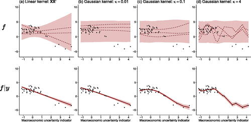
To see how a GP regression captures a possibly nonlinear relationship between y_t and x_t, Figure 1 shows the functional relationship between output growth and lagged macroeconomic uncertainty. If $\kappa =0.01$, the regression relationship is almost linear and suggests that high levels of (lagged) macroeconomic uncertainty are accompanied by negative output growth rates. When we set $\kappa =0.1$ we observe much more curvature (both in the prior and the posterior) in the relationship, indicating that if uncertainty is between 0 and around 1.7, GDP growth is between 2.3% and 2.5%. However, once a certain threshold in the first lag of uncertainty is reached, the relationship becomes strongly negative until it becomes essentially flat for very high levels of uncertainty. A similar finding, but slightly more pronounced, arises if we set κ = 4. In this case GDP growth does not change much as long as lagged uncertainty is between 0 and 1.7 and then the relationship becomes, again, strongly negative.

As is clear from this stylized example, the role of the kernel and its hyperparameters crucially impacts the posterior estimates of the function f. Setting κ too small leads to a model which might miss important (higher frequency) information whereas a κ set too large translates into an overfitting model which might yield a very strong in-sample fit but poor ouf-of-sample predictions. Setting κ is thus of crucial importance and in all our empirical work we will infer it through Bayesian updating. More information is provided in Section 3.3. After having provided the necessary foundations on Gaussian process regression, we will now focus on developing a model that is suitable for macroeconomic analysis.

3 Large-Dimensional Gaussian Process VARs

3.1 The Gaussian Process VAR

In the following discussion, let ${\mathit{y}}_t=(y_{1t},\dots ,y_{\mathit{\text{Mt}}})\prime$ denote an $M\times 1$ vector of macroeconomic and financial variables.⁶ Moreover, ${\mathit{x}}_t=(\mathit{x}{\prime }_{1t},\dots ,\mathit{x}{\prime }_{\mathit{\text{Mt}}})\prime$ denotes an $\mathit{\text{Mp}}\times 1$ vector with ${\mathit{x}}_{\mathit{\text{jt}}}=(y_{\mathit{\text{jt}}-1},\dots ,y_{\mathit{\text{jt}}-p})\prime$ storing the “own” lags of the jth endogenous variable and ${\mathit{z}}_t=(\mathit{z}{\prime }_{1t},\dots ,\mathit{z}{\prime }_{\mathit{\text{Mt}}})\prime$ an $(M-1)\mathit{\text{Mp}}\times 1$ vector of “other” lags. Hence, ${\mathit{z}}_{\mathit{\text{jt}}}=(\mathit{y}{\prime }_{-\mathit{\text{jt}}-1},\dots ,\mathit{y}{\prime }_{-\mathit{\text{jt}}-p})\prime$, where ${\mathit{y}}_{-\mathit{\text{jt}}}$ denotes the vector ${\mathit{y}}_t$ with the jth element excluded.

We discriminate between own and other lags of ${\mathit{y}}_t$ because we assume that lags of other endogenous variables impact a given endogenous variable differently from its own lags. As opposed to the literature on Bayesian VARs (see Bańbura, Giannone, and Reichlin 2010; Koop 2013; Huber and Feldkircher 2019; Chan 2021) that shrink coefficients related to own and other lags differently, we introduce more flexibility by allowing for different properties of the functions relating own and other lags to the respective outcomes.

This is achieved through two latent processes: one driven by ${\mathit{x}}_t$ and one by ${\mathit{z}}_t$. The structural form of the resulting GP-VAR is then given by (2) $${\mathit{y}}_t=F({\mathit{x}}_t)+G({\mathit{z}}_t)+\mathit{Q}{\mathit{y}}_t+{\mathit{\epsilon }}_t,\hspace{1em}{\mathit{\epsilon }}_t\sim \mathcal{N}({\mathit{0}}_M,{\mathit{H}}_t),$$(2) with $F({\mathit{x}}_t)=(f_1({\mathit{x}}_{1t}),\dots ,f_M({\mathit{x}}_{\mathit{\text{Mt}}}))\prime$ and $G({\mathit{z}}_t)=(g_1({\mathit{z}}_{1t}),\dots ,g_M({\mathit{z}}_{\mathit{\text{Mt}}}))\prime$ and f_j and g_j being equation-specific functions. The function f_j controls how y_jt depends on its own lags while g_j encodes the relationship between y_jt and the lags of the other endogenous variables. The functions f_j and g_j, and hence F and G, differ because we construct different kernels with distinct hyperparameters.⁷ This specification allows us to capture situations where the relationship between y_jt and its lags might be smooth but elements in ${\mathit{z}}_{\mathit{\text{jt}}}$ could, for example, trigger a more abrupt effect on the mean of y_jt. Or cases where there might be a linear effect between the response and its own lags but nonlinear effects induced through other lags.

The matrix $\mathit{Q}$ is an M × M lower triangular matrix with zeros along its main diagonal. This matrix defines the contemporaneous relations across the elements in ${\mathit{y}}_t$. Finally, ${\mathit{\epsilon }}_t$ is an $M\times 1$ vector of Gaussian shocks with zero mean and an M × M time-varying variance-covariance matrix ${\mathit{H}}_t=\text{diag}({\omega }_{1t},\dots ,{\omega }_{\mathit{\text{Mt}}})$. We will assume that $h_{\mathit{\text{jt}}}=\hspace{0.17em}\mathrm{\text{log}}\hspace{0.17em}{\omega }_{\mathit{\text{jt}}}$ evolves according to an AR(1) process. Allowing for time variation in the shock variances provides additional flexibility and enables to capture non-Gaussian features in the shocks (not only, but also since h_jt enters the model nonlinearly).⁸ In the Online Appendix, we show that adding SV tends to improve forecasts for U.S. macro data, whereas for the structural analysis in this article, dropping SV only has small effects on the estimated impulse response functions.

In principle, we could also allow for unknown functional relations between the contemporaneous terms of the preceding j – 1 equations and the response of equation j. However, this would lead to a complicated nonlinear covariance structure. Since we are interested in carrying out structural identification based on zero impact restrictions we opt for choosing this simpler approach which implies multivariate Gaussian reduced form shocks, but with a time-varying covariance matrix. Given that the literature on GPs typically assumes the shocks to be Gaussian and homoscedastic, this is already a substantial increase in flexibility.⁹

The model in (2) assumes that the shocks in ${\mathit{\epsilon }}_t$ are, conditional on $\mathit{Q}{\mathit{y}}_t$, orthogonal and hence estimation can be carried out equation-by-equation. We will exploit this representation for simplicity and computational tractability. The jth equation, in terms of full-data matrices, is given by $${\mathit{Y}}_j={\mathit{f}}_j+{\mathit{g}}_j+\sum _{k=1}^{j-1}{q}_{\mathit{\text{jk}}}{\mathit{Y}}_k+{\mathit{ϵ}}_j,\hspace{1em}{\mathit{ϵ}}_j\sim \mathcal{N}\left({\mathit{0}}_T,{\mathbf{\Omega }}_{\mathit{j}}\right),$$with ${\mathit{Y}}_j=(y_{j1},\dots ,y_{\mathit{\text{jT}}})\prime ,{\mathit{f}}_j=(f_j({\mathit{x}}_{j1}),\dots ,f_j({\mathit{x}}_{\mathit{\text{jT}}}))\prime$, ${\mathit{g}}_j=(g_j({\mathit{z}}_{j1}),\dots ,g_j({\mathit{z}}_{\mathit{\text{jT}}}))\prime$, q_jk denoting the (j, k)th element of $\mathit{Q},{\mathit{ϵ}}_j=({\epsilon }_{j1},\dots ,{\epsilon }_{\mathit{\text{jT}}})\prime$ and ${\mathbf{\Omega }}_{\mathit{j}}=\text{diag}({\omega }_{j1},\dots ,{\omega }_{\mathit{\text{jT}}})$. We will use this form to carry out inference about the unknown functions f_j and g_j as well as the remaining parameters and latent states of the model.¹⁰

3.2 Conjugate Gaussian Process Priors

In this section, our focus will be on the priors on f_j and g_j. The priors on the remaining, linear quantities are standard and thus not discussed in depth. We use a Horseshoe prior (Carvalho, Polson, and Scott 2010) on the free elements in $\mathit{Q}$, while for the AR(1) process of the log-volatilities h_jt a Beta prior on the (transformed) persistence parameter $({\rho }_{\mathit{\text{hj}}}+1)/2\sim \mathcal{B}(25,5)$, and an inverse Gamma prior on the state innovation variances ${\sigma }_{\mathit{\text{hj}}}^2$. This prior is specified to have mean 0.1 and variance 0.01.

For equation-specific functions f_j and g_j, we specify two GPs with one conditional on ${\mathit{X}}_j=({\mathit{x}}_{j1},\dots ,{\mathit{x}}_{\mathit{\text{jT}}})\prime$ and one conditional on ${\mathit{Z}}_j=({\mathit{z}}_{j1},\dots ,{\mathit{z}}_{\mathit{\text{jT}}})\prime$: (3) $$\begin{array}{cc}{\mathit{f}}_j\hfill & \sim \mathcal{N}\left({\mathit{0}}_T,\sqrt{{\mathbf{\Omega }}_{\mathit{j}}}{K}_{{\mathit{\vartheta }}_{j1}}({\mathit{X}}_j,{\mathit{X}}_j)\sqrt{{\mathbf{\Omega }}_{\mathit{j}}}\right),\hfill \\ {\mathit{g}}_j\hfill & \sim \mathcal{N}\left({\mathit{0}}_T,\sqrt{{\mathbf{\Omega }}_{\mathit{j}}}{K}_{{\mathit{\vartheta }}_{j2}}({\mathit{Z}}_j,{\mathit{Z}}_j)\sqrt{{\mathbf{\Omega }}_{\mathit{j}}}\right).\hfill \end{array}$$(3)

We let $\sqrt{{\mathbf{\Omega }}_{\mathit{j}}}=\text{diag}(\sqrt{{\omega }_{j1}},\dots ,\sqrt{{\omega }_{\mathit{\text{jT}}}})$ while $K_{{\mathit{\vartheta }}_{j1}}({\mathit{X}}_j,{\mathit{X}}_j)$ and $K_{{\mathit{\vartheta }}_{j2}}({\mathit{Z}}_j,{\mathit{Z}}_j)$ denote two suitable kernels with typical elements given by $$\begin{array}{cc}{k}_{{\mathit{\vartheta }}_{j1}}({\mathit{x}}_{\mathit{\text{jt}}},{\mathit{x}}_{j\tau })\hfill & ={\xi }_{j1}\times \hspace{0.17em}\mathrm{\text{exp}}\hspace{0.17em}\left(-\frac{{\kappa }_{j1}}{2}({\mathit{x}}_{\mathit{\text{jt}}}-{\mathit{x}}_{j\tau })\prime {\mathit{D}}_{{\mathit{X}}_j}^{-1}({\mathit{x}}_{\mathit{\text{jt}}}-{\mathit{x}}_{j\tau })\right),\hfill \\ \hfill & \hspace{1em}{\mathit{\vartheta }}_{j1}=({\xi }_{j1},{\kappa }_{j1})\prime ,\hfill \\ k_{{\mathit{\vartheta }}_{j2}}({\mathit{z}}_{\mathit{\text{jt}}},{\mathit{z}}_{j\tau })\hfill & ={\xi }_{j2}\times \hspace{0.17em}\mathrm{\text{exp}}\hspace{0.17em}\left(-\frac{{\kappa }_{j2}}{2}({\mathit{z}}_{\mathit{\text{jt}}}-{\mathit{z}}_{j\tau })\prime {\mathit{D}}_{{\mathit{Z}}_j}^{-1}({\mathit{z}}_{\mathit{\text{jt}}}-{\mathit{z}}_{j\tau })\right),\hfill \\ \hfill & \hspace{1em}{\mathit{\vartheta }}_{j2}=({\xi }_{j2},{\kappa }_{j2})\prime .\hfill \end{array}$$

For $j=1,\dots ,M,{\mathit{\vartheta }}_{j1}$ and ${\mathit{\vartheta }}_{j2}$ are equation and kernel-specific hyperparameters and the matrices ${\mathit{D}}_{{\mathit{X}}_j},{\mathit{D}}_{{\mathit{Z}}_j}$ are diagonal matrices with typical ith element ${\widehat{\sigma }}_{{\mathit{X}}_{j}i}^2,{\widehat{\sigma }}_{{\mathit{Z}}_{j}i}^2$. These are set equal to the empirical variances of the ith column of ${\mathit{X}}_j$ and ${\mathit{Z}}_j$, respectively. Inclusion of the diagonal scaling matrices ${\mathit{D}}_{{\mathit{X}}_j}$ and ${\mathit{D}}_{{\mathit{Z}}_j}$ serves to control for differences in the scaling of the explanatory variables. Notice that since the hyperparameters are allowed to differ, we essentially treat own and other lags asymmetrically through different functional approximations f_j and g_j.

The kernel is scaled with the error variances in ${\mathbf{\Omega }}_j$. A typical diagonal element of the corresponding rescaled kernel is given by ${\omega }_{\mathit{\text{jt}}}\times k_{{\mathit{\vartheta }}_{j1}}({\mathit{x}}_{\mathit{\text{jt}}},{\mathit{x}}_{\mathit{\text{jt}}})={\omega }_{\mathit{\text{jt}}}{\xi }_{j1}$ and ${\omega }_{\mathit{\text{jt}}}\times k_{{\mathit{\vartheta }}_{j2}}({\mathit{z}}_{\mathit{\text{jt}}},{\mathit{z}}_{\mathit{\text{jt}}})={\omega }_{\mathit{\text{jt}}}{\xi }_{j2}$. Typical off-diagonal elements are given by $\sqrt{{\omega }_{\mathit{\text{jt}}}}\sqrt{{\omega }_{j\tau }}\times k_{{\mathit{\vartheta }}_{j1}}({\mathit{x}}_{\mathit{\text{jt}}},{\mathit{x}}_{j\tau })$ and $\sqrt{{\omega }_{\mathit{\text{jt}}}}\sqrt{{\omega }_{j\tau }}\times k_{{\mathit{\vartheta }}_{j2}}({\mathit{z}}_{\mathit{\text{jt}}},{\mathit{z}}_{j\tau })$. The interaction between the kernel and the error variances gives rise to convenient statistical and computational properties.

First, note that if ω_jt is large, the corresponding prior on the unknown functions is more spread out. In macroeconomic data, ω_jt is typically elevated in crisis periods when ${\mathit{x}}_{\mathit{\text{jt}}}$ and ${\mathit{z}}_{\mathit{\text{jt}}}$ are far away from their previous values. Since the diagonal elements of the kernels are effectively determined by ${\mathit{\xi }}_j=({\xi }_{j1},{\xi }_{j2})\prime$ the presence of ω_jt allows for larger values in the marginal prior variance and thus makes large shifts in the unknown functions more likely. Second, the interaction between ω_jt and ${\omega }_{\mathit{\text{jt}}-1}$ implies that the covariances are scaled down if ${\omega }_{\mathit{\text{jt}}}\gg {\omega }_{\mathit{\text{jt}}-1}$, suggesting that the informational content decreases if increases in uncertainty are substantial (i.e., $\Delta {\omega }_{\mathit{\text{jt}}}$ is large). If ${\omega }_{\mathit{\text{jt}}}\approx {\omega }_{j\tau }$ and both are large, the corresponding covariance will be scaled upwards. This implies that our model learns from previous crisis episodes as well. Third, as we will show in Section 3.4, interacting the kernel with the error variances leads to a conjugate Gaussian process structure which implies that we can factor out the error volatilities and do not need to update several quantities during MCMC sampling. This speeds up computation enormously and allows for estimating large models.

3.3 Selecting the Hyperparameters Associated with the Kernel

So far, we always conditioned on the hyperparameters that determine the shape of the Gaussian kernel. A simple way of specifying ${\mathit{\vartheta }}_{j1}$ and ${\mathit{\vartheta }}_{j2}$ is the median heuristic approach stipulated in Chaudhuri et al. (2017). This choice works well in a wide range of applications featuring many covariates (see, e.g., Crawford et al.2019). The median heuristic fixes ${\xi }_{j1}={\xi }_{j2}=1$ and defines the inverse of the bandwidth parameter as $$\begin{array}{cc}{\kappa }_{j1}\hfill & ={\overline{\kappa }}_{j1}={\text{median}}_{t\tau }\left(\frac{1}{\Vert {\mathit{x}}_{\mathit{\text{jt}}}-{\mathit{x}}_{j\tau }\Vert }\right),\hfill \\ {\kappa }_{j2}\hfill & ={\overline{\kappa }}_{j2}={\text{median}}_{t\tau }\left(\frac{1}{\Vert {\mathit{z}}_{\mathit{\text{jt}}}-{\mathit{z}}_{j\tau }\Vert }\right),\hfill \end{array}$$for $j=1,\dots ,M$. This simple approach has the convenient property that it automatically selects a bandwidth which is consistent with the time series behavior of the elements in ${\mathit{y}}_t$. To illustrate this, suppose that y_jt is a highly persistent process (e.g., inflation or short-term interest rates). In this case, for $\tau =t-1$, the Euclidean distance $\Vert {\mathit{x}}_{\mathit{\text{jt}}}-{\mathit{x}}_{j\tau }\Vert$ will be quite small and, hence, the mean function ${\mathit{f}}_j$ smoothly adjusts. If y_jt is less persistent and displays large fluctuations (e.g., stock market or exchange rate returns), the Euclidean distance $\Vert {\mathit{x}}_{\mathit{\text{jt}}}-{\mathit{x}}_{j\tau }\Vert$ will be large and, thus, ${\mathit{f}}_j$ allows for capturing this behavior. The dispersion in ${\mathit{z}}_{\mathit{\text{jt}}}$ might have important implications for y_jt if the aim is to model a trend in y_jt that depends on other covariates. This could arise in a situation where the prior on ${\mathit{f}}_j$ is set very tight (i.e., the posterior of ${\mathit{f}}_j$ will be centered on zero) and information not coming from ${\mathit{x}}_{\mathit{\text{jt}}}$ would then determine the behavior of y_jt. This discussion highlights how the median heuristic allows for flexibly discriminating between signal and noise and thus acts as a nonlinear filter which purges the time series from high frequency variation, if necessary.

Given that we work with potentially large panels of time series, it is questionable that the median heuristic works equally well for all elements in ${\mathit{y}}_t$. As a solution, we propose to use the median heuristic to set up a discrete grid for both ${\xi }_{j1}$ (${\xi }_{j2}$) and ${\kappa }_{j1}$ (${\kappa }_{j2}$). For each element in this grid we specify a hyperprior. We use Gamma priors on all elements. For $j=1,\dots ,M$, that is, $${\xi }_{j1}\sim \mathcal{G}\left(\frac{1}{2},\frac{1}{2c_{\xi 1}}\right)\hspace{1em}\text{and}\hspace{1em}{\xi }_{j2}\sim \mathcal{G}\left(\frac{1}{2},\frac{1}{2c_{\xi 2}}\right),$$

for the linear shrinkage hyperparameters and $${\kappa }_{j1}\sim \mathcal{G}\left(\frac{1}{2},\frac{1}{2c_{\kappa 1}}\right)\hspace{1em}\text{and}\hspace{1em}{\kappa }_{j2}\sim \mathcal{G}\left(\frac{1}{2},\frac{1}{2c_{\kappa 2}}\right),$$for the bandwidth parameters. Here, $c_{\xi 1},c_{\xi 2},c_{\kappa 1}$ and $c_{\kappa 2}$ are scalars defining the tightness of the hyperprior. In the empirical application, we set $c_{\xi 1}=c_{\xi 2}=c_{\xi }$ and $c_{\kappa 1}=c_{\kappa 2}=c_{\kappa }$. These parameters strongly influence the shape of the conditional mean and are crucial modeling choices: we set them through cross-validation. In our empirical application, we find that small values of $c_{\kappa }$ work well, yielding an informative prior that forces ${\kappa }_{j1}$ and ${\kappa }_{j2}$ toward zero.

Based on this set of priors we can derive the conditional posterior distribution. Since ${\xi }_{j1}$ (${\xi }_{j2}$) and ${\kappa }_{j1}$ (${\kappa }_{j2}$) are placed on a grid, we can pre-compute several quantities related to the kernel (such as inverses and Cholesky factors) while at the same time infer them from the data with sufficient accuracy, which is crucial for precise inference. We center these grids around the median heuristic and additionally take into account the considerations of the informative Gamma priors: $${\kappa }_{\mathit{\text{jk}}}\in [0.1{\overline{\kappa }}_{\mathit{\text{jk}}},2{\overline{\kappa }}_{\mathit{\text{jk}}}]\hspace{1em}\text{and}\hspace{1em}{\xi }_{\mathit{\text{jk}}}\in [0.04,4],$$ $$\hspace{1em}\text{for}j=1,\dots ,M\text{and}k=1,2.$$

Here, the intervals indicate the minimum (maximum) value supported for each hyperparameter. Within this two dimensional range, we define a discrete grid of around 1,000 combinations with equally sized increments along each dimension.¹¹ The corresponding posterior is discrete and we can use inverse transform sampling to carry out posterior inference. Further details are provided in Section 3.4.

3.4 Posterior Computation

Posterior inference for the GP-VAR is carried out using a novel yet conceptually simple MCMC algorithm which cycles between several steps. In this section we will focus on how to sample from the posterior of ${\mathit{f}}_j,p({\mathit{f}}_j|•)$, with $•$ denoting conditioning on everything else, and ${\mathit{\vartheta }}_{j1}$. Sampling from $p({\mathit{g}}_j|•)$ and $p({\mathit{\vartheta }}_{j2}|•)$ works analogously with some adjustments. These relate to the fact that we introduce a linear restriction that ${(\mathit{\iota }\prime \mathit{\iota })}^{-1}\mathit{\iota }\prime {\mathit{g}}_j=0$, with $\mathit{\iota }$ denoting a $T\times 1$ vector of ones. The corresponding conditional posterior distribution is a hyperplane truncated Gaussian where efficient sampling algorithms are available (see Cong, Chen, and Zhou 2017). Further details can be found in Section A.3 of the Online Appendix.

It is worth stressing that we sample ${\mathit{f}}_j$ and ${\mathit{g}}_j$ separately. This increases the computational burden slightly but allows us to consider both latent processes separately from each other. The posterior of ${\mathit{f}}_j$ is Gaussian for all j: $$\begin{array}{cc}\hfill & {\mathit{f}}_j|•\sim \mathcal{N}({\overline{\mathit{f}}}_j,{\overline{\mathit{V}}}_{{\mathit{f}}_j}),\hspace{1em}\text{with posterior moments given by}\hfill \\ {\overline{\mathit{V}}}_{{\mathit{f}}_j}=\hfill & \sqrt{{\mathbf{\Omega }}_{\mathit{j}}}(K_{{\mathit{\vartheta }}_{j1}}({\mathit{X}}_j,{\mathit{X}}_j)-K_{{\mathit{\vartheta }}_{j1}}({\mathit{X}}_j,{\mathit{X}}_j){\left(K_{{\mathit{\vartheta }}_{j1}}({\mathit{X}}_j,{\mathit{X}}_j)+{\mathit{I}}_T\right)}^{-1}\hfill \\ \hfill & K_{{\mathit{\vartheta }}_{j1}}({\mathit{X}}_j,{\mathit{X}}_j))\sqrt{{\mathbf{\Omega }}_{\mathit{j}}},\hfill \\ {\overline{\mathit{f}}}_j=\hfill & \sqrt{{\mathbf{\Omega }}_{\mathit{j}}}{K}_{{\mathit{\vartheta }}_{j1}}({\mathit{X}}_j,{\mathit{X}}_{\mathit{j}}){\left(K_{{\mathit{\vartheta }}_{j1}}({\mathit{X}}_j,{\mathit{X}}_j)+{\mathit{I}}_T\right)}^{-1}\hfill \\ \hfill & \mathrm{\hspace{1em}}\mathrm{\hspace{1em}}{\sqrt{{\mathbf{\Omega }}_{\mathit{j}}}}^{-1}\left({\mathit{Y}}_j-{\mathit{g}}_j-\sum _{k=1}^{j-1}{q}_{\mathit{\text{jk}}}{\mathit{Y}}_k\right),\hfill \end{array}$$where for j = 1, the term ${\sum }_{k=1}^{j-1}{q}_{\mathit{\text{jk}}}{\mathit{Y}}_k$ is excluded.

In principle, computing the inverse and the Cholesky factor of ${\overline{\mathit{V}}}_{{\mathit{f}}_j}^{-1}$ constitutes the main bottleneck when sampling from $p({\mathit{f}}_j|•)$. This is especially so if T is large. But, in common macroeconomic applications which use quarterly data, T is moderate and thus computation is feasible. In our case, even if interest centers on using monthly data or even higher frequencies, we can exploit the convenient fact that, conditional on the hyperparameters ${\xi }_{j1}$ and ${\kappa }_{j1}$, $${\mathit{B}}_{{\mathit{f}}_j}\mathit{B}{\prime }_{{\mathit{f}}_j}=(K_{{\mathit{\vartheta }}_{j1}}({\mathit{X}}_j,{\mathit{X}}_j)-K_{{\mathit{\vartheta }}_{j1}}({\mathit{X}}_j,{\mathit{X}}_j){\left(K_{{\mathit{\vartheta }}_{j1}}({\mathit{X}}_j,{\mathit{X}}_j)+{\mathit{I}}_T\right)}^{-1}$$ $$\mathrm{\hspace{1em}}\mathrm{\hspace{1em}}{K}_{{\mathit{\vartheta }}_{j1}}({\mathit{X}}_j,{\mathit{X}}_j))$$

as well as its Cholesky factor ${\mathit{B}}_{{\mathit{f}}_j}$ can be pre-computed. In addition, notice that $${\overline{\mathit{V}}}_{{\mathit{f}}_j}={\mathit{C}}_{{\mathit{f}}_j}\mathit{C}{\prime }_{{\mathit{f}}_j}=\left(\sqrt{{\mathbf{\Omega }}_{\mathit{j}}}{\mathit{B}}_{{\mathit{f}}_j}\right)\left(\sqrt{{\mathbf{\Omega }}_{\mathit{j}}}{\mathit{B}}_{{\mathit{f}}_j}\right)\prime .$$

These practical properties (due to the conjugate structure) substantially speed up computation in terms of sampling from $p({\mathit{f}}_j|•)$.

These results are conditional on the hyperparameters. As outlined in the previous section, we will estimate them by defining a discrete two dimensional grid of 1,000 combinations. For each hyperparameter combination on this grid, we compute the corresponding kernel $K_{{\mathit{\vartheta }}_{j1}}({\mathit{X}}_j,{\mathit{X}}_j)$ as well as all relevant quantities (i.e., ${\mathit{C}}_{{\mathit{f}}_j}$). Based on these values we jointly evaluate the conditional posterior by applying Bayes’ theorem. The conditional likelihood is proportional to $$\begin{array}{cc}p({\mathit{f}}_j|{\mathit{\vartheta }}_{j1},{\mathbf{\Omega }}_{\mathit{j}})\hfill & \propto \text{det}{\left(\sqrt{{\mathbf{\Omega }}_{\mathit{j}}}{K}_{{\mathit{\vartheta }}_{j1}}({\mathit{X}}_j,{\mathit{X}}_j)\sqrt{{\mathbf{\Omega }}_{\mathit{j}}}\right)}^{-\frac{1}{2}}\hfill \\ \hfill & \hspace{1em}\times \hspace{0.17em}\mathrm{\text{exp}}\hspace{0.17em}\mathrm{}\left\{-\frac{1}{2}\left({\mathit{f}}_j^{\prime }{\left(\sqrt{{\mathbf{\Omega }}_{\mathit{j}}}{K}_{{\mathit{\vartheta }}_{j1}}({\mathit{X}}_j,{\mathit{X}}_j)\sqrt{{\mathbf{\Omega }}_{\mathit{j}}}\right)}^{-1}\mathrm{}{\mathit{f}}_j\right)\right\}.\hfill \end{array}$$

Note that the shape of $K_{{\mathit{\vartheta }}_{j1}}({\mathit{X}}_j,{\mathit{X}}_j)$ depends on the hyperparameters ${\mathit{\vartheta }}_{j1}=({\xi }_{j1},{\kappa }_{j1})\prime$, which we want to update. For each pair of values ${\mathit{\vartheta }}_{j1}^{(s)}$ on our two dimensional grid (with s denoting a specific combination), we compute the corresponding kernel $K_{{\mathit{\vartheta }}_{j1}={\mathit{\vartheta }}_{j1}^{(s)}}({\mathit{X}}_j,{\mathit{X}}_j)$ as well as $\text{det}(K_{{\mathit{\vartheta }}_{j1}={\mathit{\vartheta }}_{j1}^{(s)}}({\mathit{X}}_j,{\mathit{X}}_j))$ and ${(K_{{\mathit{\vartheta }}_{j1}={\mathit{\vartheta }}_{j1}^{(s)}}({\mathit{X}}_j,{\mathit{X}}_j))}^{-1}$ prior to MCMC sampling. Hence, within our sampler evaluating the likelihood is straightforward and computationally efficient. All that remains is to multiply the likelihood with the prior. The corresponding posterior ordinates for each ${\mathit{\vartheta }}_{j1}^{(s)}$ are used to compute probabilities to perform inverse transform sampling to sample from $p({\mathit{\vartheta }}_{j1}|•)$.

Conditional on ${\mathit{f}}_j$ and ${\mathit{g}}_j$, the remaining parameters (i.e., the free elements in $\mathit{Q}$, the log-volatilities and the associated coefficients in the corresponding state equations) can be sampled through (mostly) standard steps. One modification relates to how we sample the volatilities in ${\mathbf{\Omega }}_{\mathit{j}}$. The main difference stems from the fact that the volatilities in ${\mathbf{\Omega }}_{\mathit{j}}$ also show up in the prior on ${\mathit{f}}_j$ and ${\mathit{g}}_j$. To circumvent this issue we integrate out the latent processes ${\mathit{f}}_j$ and ${\mathit{g}}_j$. This calls for a minor adjustment of the original sampler by integrating out the latent processes ${\mathit{f}}_j$ and ${\mathit{g}}_j$ first and then sampling the log-volatilities using an independent Metropolis Hastings update similar to the one proposed in Chan (2017). We provide additional details and the full posterior simulator in Section A of the Online Appendix. In our empirical work, we focus on generalized impulse response functions (GIRFs) and we show in Sections A.6 and A.7 of the Online Appendix how we compute them.

We now illustrate that our approach is computationally efficient and scalable to large datasets. Figure 2 shows the time required to generate $1,000$ draws from the joint posterior for a particular equation across different values of K and for T = 200.¹² We show the computation times for our GP-VAR and a linear BVAR with SV. To ensure comparability between both models, we estimate the linear BVAR model on an equation-by-equation basis as well. Since we can parallelize this system of multiple equations for both approaches, the actual times for generating 1,000 draws from the joint posterior of the full system are approximately M times the run times reported in the figure for both the GP-VAR and the BVAR.¹³

Fig. 2 Computation time for 1,000 draws from the joint posterior distribution.

NOTE: Computation times for 1,000 draws from the joint posterior distribution of a standard BVAR (black) and the GP-VAR (orange), across a varying number of regressors, K. In a VAR, typically K = Mp for each individual equation, where M represents the number of included endogenous variables, and p denotes the number of lags. Since we can parallelize this system of multiple equations for both approaches, the actual times for generating 1,000 draws from the joint posterior of the full system is approximately M times the run times reported in this figure for both the GP-VAR and the BVAR. Computation times are based on a desktop machine with an AMD Ryzen 7 5800X 8-Core processor.

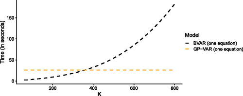
The figure strikingly shows that the computation time of the GP-VAR does not depend on K. By contrast, the time necessary to generate a draw from the joint posterior of the VAR rises rapidly in K. Hence, our approach can be used if K is large. To provide a rough gauge on gross estimation times (i.e., computation times that include pre-computation of certain quantities and without using parallel computing): it takes around 30 min to estimate a GP-VAR with eight endogenous variables and five lags on a standard desktop computer (for $10,000$ MCMC draws). Estimating larger models (such as the 64 variable GP-VAR) takes around four hours.

4 The Macroeconomic Effects of Uncertainty Shocks

4.1 Monte Carlo Exercise

Before we deal with real data, we examine whether our GP-VAR recovers the responses of the economy to an uncertainty shock within a controlled environment. To this end, we use the dynamic stochastic general equilibrium (DSGE) model proposed in Basu and Bundick (2017) to simulate time series of length T = 120 and use these to back out the responses of the model economy to unexpected shocks in uncertainty. The Basu and Bundick (2017) model is a dynamic DSGE model that features optimizing households and companies and assumes that the central bank sets interest rates according to a Taylor rule. The observed variables are output (GDP), consumption (CONS), investment (INV), hours worked (HWORK), inflation, M2 money stock, and the implied stock market volatility (VXO).

We simulate 50 realizations from the theoretical DSGE data-generating process (DGP). For each realization, we estimate our nonparametric GP-VAR model and compare its responses not only to the true underlying DSGE responses but also with those obtained from a classical linear BVAR. The uncertainty shock is identified by ordering the stock market volatility (our measure of uncertainty) first, implying an immediate reaction of all real economic quantities in the system following an uncertainty shock. This identification scheme is fully supported by the DSGE model (see sec. 7.5 in Basu and Bundick,2017 for a discussion).

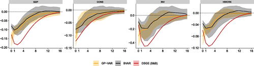
We start by illustrating that our model produces dynamic reactions consistent with the DSGE-based IRFs. In Figure 3 we plot the theoretical IRFs (in red), the GP-VAR GIRFs (in orange) and the BVAR IRFs (in gray) for four variables (GDP, CONS, INV, HWORK). The solid lines are averages of posterior medians of the (G)IRFs, while the bounds denote the 16th and 84th percentiles of the posterior medians over the 50 replications from the DGP. In terms of qualitative statements, the GP-VAR produces GIRFs that are consistent with the theoretical predictions from the structural model. In response to an uncertainty shock, real activity (and its components) declines. However, both the GP-VAR and the BVAR produce impulse responses which are less persistent than the ones of the DSGE model. Notice that the GP-VAR produces immediate reactions which are much closer to the model-implied responses for all variables except for investments.

Fig. 3 Summary of posterior median responses across 50 simulations from the DSGE model proposed in Basu and Bundick (2017).

NOTE: Average generalized impulse responses (GIRFs, outlined in Section A.7 of the Online Appendix) to a positive one standard deviation shock in implied stock market volatility. The responses estimated with our nonparameteric GP-VAR model are shown in orange, while responses estimated with a BVAR model are shown in gray. The theoretical responses implied by the DSGE model proposed in Basu and Bundick (2017 ) are shown in red. Solid lines are averages of posterior medians of the responses, while shaded areas denote the range between the 16th and 84th percentiles of the posterior medians over the 50 replications from the DGP.

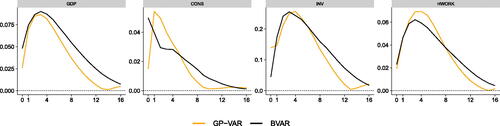
To obtain a better quantitative feeling on whether our proposed model improves upon the linear BVAR, we report root mean squared errors (RMSEs) between the posterior median of the IRFs of a given model and the DSGE-based IRFs for each horizon in Figure 4. These RMSE curves are, again, averages over the 50 simulations from the theoretical Basu and Bundick (2017) model. From this figure we learn that the GP-VAR produces lower RMSEs for almost all forecast horizons for output and investments. For consumption our model sharply improves upon the linear VAR on impact and for horizons greater than seven quarters but is outperformed in between. Finally, for hours worked we find that in terms of RMSEs, both models produce similar IRFs that only differ in their short-run reactions. After showing that our model works reasonably well within a controlled environment, we now turn to the real data application.

Fig. 4 Root mean squared errors (RMSEs) across 50 simulations relative to the theoretical Basu and Bundick (2017) responses over the impulse response horizons.

NOTE: The figure depicts the root mean squared errors (RMSEs) across 50 simulations, benchmarking the posterior median responses of the GP-VAR and the BVAR against the theoretical responses implied by the DSGE model proposed in Basu and Bundick (2017 ). RMSEs of our nonparametric GP-VAR model are shown in orange, while RMSEs of the BVAR model are shown in black.

4.2 Data Overview and Model Specification

We use the quarterly version of the dataset in McCracken and Ng (2016) for the period 1960Q1 to 2019Q4. We exclude the years of the Covid-19 pandemic to make the comparison with a linear VAR similar to that used in Jurado, Ludvigson, and Ng (2015) (JLN) sensible. We consider four different specifications that differ in the number of endogenous variables used. These specifications are:

GP-VAR-8: This dataset is patterned after the original JLN dataset. It includes the JLN macroeconomic uncertainty index (labeled as UNC), real GDP (RGDP), civilian employment (EMP), average weekly working hours in manufacturing (AWH), consumer price index (CPI), average hourly earnings in manufacturing (AHE), Fed funds rate (FFR), and the S&P 500 (SP500).

GP-VAR-16: In addition to the variables in the VAR with M = 8 endogenous variables, we also include the components of GDP (such as real personal consumption and real private fixed investment), additional labor market variables (such as unemployment, initial claims, average weekly working hours and average hourly earnings across all sectors), housing starts, as well as the real M2 money stock.

GP-VAR-32: On top of the variables of the VAR with M = 16 variables, we include important financial variables, further data on housing and data on loans.

GP-VAR-64: The largest model we consider features M = 64 endogenous variables. The set of endogenous variables is obtained by taking the variables with M = 32 and including additional financial variables and data on manufacturing.

All variables are transformed to be approximately stationary and we include five lags of the endogenous variables. Using five lags is a standard choice and motivated by the wish to capture dynamics over the full last year (see, e.g., Carriero, Clark, and Marcellino 2015). The precise variables included (and transformations applied to each variable) are shown in Table B.1 in the Online Appendix. We consider these different model sizes for several reasons. First, we would like to assess how adding additional information impacts the forecasting performance and the responses of key variables to an uncertainty shock. Second, we are interested in the relationship between nonlinearities and the size of the model.

Table 1 Correlation between key macroeconomic variables and asymmetry measures.

	Sign		Size
	D	DC	D	DC
Focus variables
UNC	–0.46	–0.78	–0.14	–0.26
RGDP	0.60	0.47	0.52	0.27
EMP	0.48	0.32	0.34	0.11
SP500	–0.18	0.02	–0.23	0.05
Other macro factors
FFR	0.63	0.44	0.66	0.45
AWH	0.78	0.80	0.73	0.74
CPI	0.70	0.55	0.70	0.59

Before we proceed with our actual empirical analysis, it is worth stressing that Section E of the Online Appendix includes additional empirical work. Most notably, this includes a forecasting exercise based on the dataset described in this section that serves to illustrate that our model generates excellent forecasts.

4.3 Comparison with Standard BVAR Analysis

We benchmark the IRFs of our GP-VAR-8 to the ones of a BVAR with SV that is closely related to the original JLN specification.¹⁴ Our focus will be on the variables discussed in JLN: year-on-year growth rates of output (measured through real GDP) and employment. These two variables are informative regarding investment and labor adjustment non-convex costs which are central in micro-founded models such as Bloom (2009) and Bloom, et al. (2018). We also show the responses of the uncertainty indicator and the quarter-on-quarter returns of the S&P 500 and include the responses of the other variables in Section E of the Online Appendix.

In Figure 5 we report the (average over time in the case of the GP-VAR) posterior quantiles (16th, 50th, 84th) of the responses to a macroeconomic uncertainty shock in the JLN model (in gray) and in the corresponding GP-VAR (in orange) with eight endogenous variables and uncertainty ordered second after stock market returns.¹⁵ Uncertainty responses to its own shock differ slightly between the GP-VAR and the linear model. These differences relate to responses within the first five quarters after the shock hits the system. The BVAR yields uncertainty reactions that peak after one quarter, declining steadily afterwards. Instead, the GP-VAR generates endogenous uncertainty reactions which peak after five quarters, declining sharply afterwards. After around eight quarters, both IRFs (almost) coincide.

Fig. 5 Impulse responses of focus variables in the GP-VAR-8 relative to a small-scale BVAR.

NOTE: Average generalized impulse responses (GIRFs, outlined in Section A.7 of the Online Appendix) to a positive one standard deviation shock in macroeconomic uncertainty. Solid lines denote the posterior medians, while shaded areas correspond to the 68% posterior credible sets. GP-VAR-8 refers to the smallest variant of our nonparametric model and BVAR-8 refers to a small-scale BVAR with SV, which is closely related to the specification used in Jurado, Ludvigson, and Ng (2015 ).

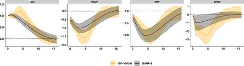
This uncertainty reaction has direct implications on how the other variables in the model react. Real GDP growth reacts in an hump-shaped manner under both models. However, driven by the somewhat later peak in uncertainty, the GP-VAR produces much stronger output growth reactions that peak slightly later (after around five quarters). When we focus on employment growth the IRFs differ less. In principle, both models suggest a peak decline of around 0.8 percentage points, with the GP-VAR generating a somewhat slower response, reaching its trough after about six to seven quarters. But in principle, responses between the linear and nonparametric model tell a similar story. Finally, financial market reactions measured through the S&P500 suggest a much stronger decline in stock prices under the GP-VAR. Interestingly, the shape of the IRFs suggests that the linear model generates the strongest reaction after around two quarters. In the GP-VAR, we find that stock markets react faster and stronger to uncertainty shocks, with substantial reactions within the first year after the shock hit the system.

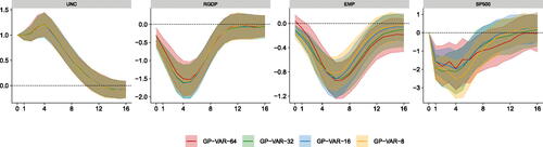
To conclude, in Figure 6 we report the GIRFs to the uncertainty shock for the same four variables displayed in Figure 5 but obtained from GP-VARs of different dimensions (with 8, 16, 32, and 64 variables). Differences across model sizes are small (or nonexistent) for most variables. Small differences arise for employment growth, with the magnitude of the responses increasing with the model size. Stock market reactions also differ slightly across datasets, with no clear-cut pattern. Since the GIRFs are very similar across model size and given its excellent forecasting properties, we will focus on asymmetries generated by the GP-VAR-8 model in the following sections. Results for the larger models are provided in the Online Appendix.

Fig. 6 Impulse responses of focus variables across different information sets.

NOTE: Average generalized impulse responses (GIRFs, outlined in Section A.7 of the Online Appendix) to a positive one standard deviation shock in macroeconomic uncertainty across different information sets. Solid lines denote the posterior medians, while shaded areas correspond to the 68% posterior credible sets.

4.4 Asymmetries in the Transmission of Uncertainty Shocks

The nonlinear and nonparametric nature of our models allows for asymmetries in the impulse response functions. This implies that shocks propagate nonlinearly through the model, giving rise to differences in the GIRFs both over time but also for different shock magnitudes or signs.

4.4.1 Asymmetries with Respect to the Sign of the Shock

We first consider whether positive and negative uncertainty shocks trigger different responses of the economy. In Figure 7 we report the responses to negative and positive uncertainty shocks from the GP-VAR-8, averaged over time. The figure thus shows GIRFs to a positive (in orange), negative (in blue) and a negative shock multiplied by –1 (in gray, to ease comparison). From the figure we observe some differences. These differences mostly relate to peak reactions as well as short-run (i.e., within two years) responses. In general, we find that positive shocks (higher uncertainty) trigger a stronger reaction of uncertainty, which in turn translates into more pronounced reactions of real activity and stock market quantities.

Fig. 7 Shock sign asymmetries in responses of focus variables for the GP-VAR-8.

NOTE: Average generalized impulse responses (GIRFs, outlined in Section A.7 of the Online Appendix) to a negative (positive) one standard deviation shock in macroeconomic uncertainty. Solid lines denote the posterior medians, while shaded areas correspond to the 68% posterior credible sets. Here, negative $\times (-1)$ denotes a negative one standard deviation shock with the respective responses being mirrored across the x-axis.

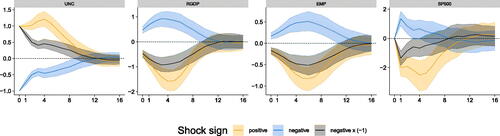
More specifically, considering the endogenous reaction of the uncertainty indicator shows that responses to a positive uncertainty shock peak after around a year and quickly die out afterwards. However, if uncertainty unexpectedly declines, the peak happens on impact and is much smaller as opposed to an adverse uncertainty shock.

Turning to real GDP and employment growth, we find that positive shocks trigger stronger reactions for both variables. Interestingly, the timing of the peak responses is similar for negative and positive shocks but reactions appear much more pronounced for the latter. Stock market reactions also differ markedly across positive and negative shocks. For positive shocks we, again, find that the peak effect happens after one year and that it is more pronounced as compared to the negative shock. Overall, the picture that emerges from the GP-VAR is that higher unexpected uncertainty has stronger effects on the economy than lower uncertainty, a feature that is a priori ruled out in linear VARs.

4.4.2 Asymmetries with Respect to the Size of the Shock

Our GP-VAR also permits to analyze how shocks of different sizes impact the economy. While in a standard VAR shocks enter linearly (and thus responses to shocks of different sizes are exactly proportional to each other), our GP-VAR is more flexible and allows for investigating whether shocks of different magnitudes trigger different dynamics in the GIRFs.

In Figure 8 we consider two shock sizes: one and two standard deviation. To permit straightforward comparison of the shapes of the responses to differently sized shocks, we also add impulses to a two standard deviation shock which are then rescaled to match the impact of the one standard deviation shock (the gray shaded area in the figures).

Fig. 8 Shock size asymmetries in responses of focus variables for the GP-VAR-8.

NOTE: Average generalized impulse responses (GIRFs, outlined in Section A.7 of the Online Appendix) to a positive two (one) standard deviation shock in macroeconomic uncertainty. Solid lines denote the posterior medians, while shaded areas correspond to the 68% posterior credible sets. Here, 1 sd refers to a one standard deviation shock, 2 sd indicates a two standard deviation shock, and 2 sd $\times (1/2)$ denotes a two standard deviation shock with the respective responses divided by two.

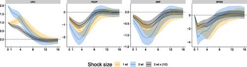
This figure gives rise to at least two observations. First, when we compare the shape of the responses to a one standard deviation to the ones of a two standard deviation shock we find differences in the timing (and more generally in the shape) of the IRFs. A stronger shock triggers a faster peak reaction of GDP and employment growth. Stock market reactions display a somewhat different shape. After a sharp immediate reaction (for both shock sizes) the peak effect happens to be on impact if the size of the shock is large whereas it turns out to materialize after one year if the shock size is smaller.

Second, in terms of the magnitudes we find that a two standard deviation shock triggers peak responses with magnitudes that are less than twice the magnitudes to a one standard deviation shock. This is particularly visible for employment and output reactions. For stock market responses, the impact reactions are (almost) proportional to each other.

4.4.3 Asymmetries over Time

After showing that the economy’s reaction depends on the sign and size of the uncertainty shock, we study whether its effects also change over time (see sec. 2.5 of Castelnuovo (2023), or Mumtaz and Theodoridis (2018) for some evidence using TVP-VARs).

We start by considering impulse responses averaged over certain sub-periods in Figure 9. The classification into sub-periods is mostly taken from D’Agostino and Surico (2012), and it is such that the main events in each sub-period include, respectively, the great inflation (1970Q1 to 1984Q4), the great moderation (1985Q1 to 2006Q4), and the post great moderation period (2007Q1 to 2019Q4). To also evaluate whether asymmetries between positive and negative shocks have changed over time, all figures include the IRFs to positive (in orange) and negative (in blue) shocks.

Fig. 9 Impulse responses of focus variables in the GP-VAR-8 across different sub-sample periods.

NOTE: Period-specific average generalized impulse responses (GIRFs, outlined in Section A.7 of the Online Appendix) to a positive (negative) one standard deviation shock in macroeconomic uncertainty. Solid lines denote the posterior medians, while shaded areas correspond to the 68% posterior credible sets.

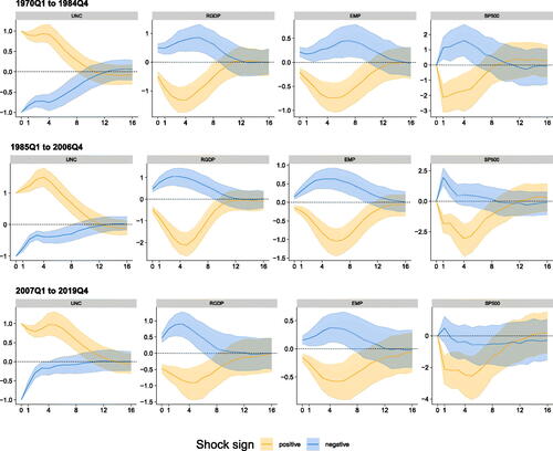
The main feature emerging from the figure is the different behavior of the response of uncertainty across sub-samples. In the final two sub-samples, uncertainty responses increase up to four quarters after the shock, with peak effects being strongest in the great moderation period and becoming slightly weaker in the final sub-sample. Moreover, sign effects of uncertainty responses increase appreciably in the last two sub-samples.

These differences in the responses of uncertainty trigger differences in the IRFs of the other quantities which relate not only to the magnitudes but also to the shapes of the responses. We find that GDP growth, employment and the S&P 500 display the strongest reactions in the great moderation regime, becoming slightly weaker in the post great moderation period. The weaker reaction of real activity over time corroborates findings in Mumtaz and Theodoridis (2018) who also report smaller responses of real activity to uncertainty shocks. As opposed to their findings, we observe that stock market reactions do not change much in magnitude but the shape differs (in accordance with the different shape in the uncertainty reaction described above). We, moreover, observe that asymmetries in terms of the sign of the shocks have decreased over time for GDP and employment growth. Only for stock market reactions these sign asymmetries have increased, with benign uncertainty shocks yielding a much weaker positive reaction of stock markets during the post great moderation regime.

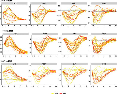
Finally, to conclude this section we raise the issue that considering GIRFs averaged over sub-samples possibly still masks important differences over time within sub-samples. To shed light on whether IRFs change within regimes, Figure 10 displays yearly averages of posterior medians of the IRFs over time during each of the three periods. Yellow IRFs refer to the beginning of the respective sub-sample and red ones denote IRFs computed toward the end of the sub-sample. This figure suggests substantial heterogeneity in responses during the great inflation period. Especially toward the end of this sample, reactions of GDP growth and employment point toward a substantial real activity overshoot. During the great moderation, the intra-period variation of the IRFs becomes much smaller, yielding patterns more consistent with the common wisdom in the uncertainty literature: real activity and stock markets decline in response to increases in economic uncertainty. In the years from 2007 to 2019, we find that IRFs differ especially in the beginning of the sample (from 2007 to 2009). For the remaining years, there is much less variation in responses and they are similar to those observed in 1985–2006.

Fig. 10 Period-specific impulse responses of focus variables in the GP-VAR-8 across different sub-sample periods.

NOTE: Generalized impulse responses (GIRFs, outlined in Section A.7 of the Online Appendix) to a positive one standard deviation shock in macroeconomic uncertainty in the GP-VAR-8 across sub-sample periods. Solid lines denote the yearly averaged posterior medians, with colors ranging from yellow (start of the sample) to red (end of the sample).

Overall, we can conclude that the effects of uncertainty change both during sub-samples defined by economic considerations and sometimes also within each sub-sample. This kind of time variation is a priori ruled out in linear VAR models, which can therefore lead to biased estimates of the effects of uncertainty.

4.5 A Deeper Look at Model-Implied Asymmetries

The previous sections focused on whether our model produces asymmetries with respect to shock size, sign and whether the transmission of uncertainty has changed over time. The analysis related to shock size and sign, however, focused on full sample asymmetries and this might mask temporal heterogeneity. For instance, it could be that sign asymmetries are more pronounced in different stages of the business cycle and thus depend on time. In this section, we focus on how asymmetries evolve over time and then compute correlations to observed macroeconomic variables to understand whether they are related.

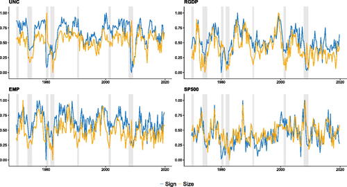
Figure 11 (and Figure E.16 in the Online Appendix) show the posterior mean of the asymmetry measures proposed in Olivei and Tenreyro (2010). These are given by $${\mathrm{D}}_t=\mathrm{\text{max}}{\Vert {\mathit{\delta }}_{\mathit{\text{ht}}}^{+}+{\mathit{\delta }}_{\mathit{\text{ht}}}^{-}\Vert }_1,\hspace{1em}{\text{DC}}_t={\Vert \sum _{h=0}^{16}({\mathit{\delta }}_{\mathit{\text{ht}}}^{+}+{\mathit{\delta }}_{\mathit{\text{ht}}}^{-})\Vert }_1.$$

Fig. 11 The normalized ${\mathrm{D}}_t$ measure for sign and size asymmetries of the key variables.

NOTE: This figure shows the normalized ${\mathrm{D}}_t$ measures, which represent the maximum absolute difference in responses over the horizon in period t. These measures are normalized to lie between zero and one. Sign asymmetries compare the differences in responses to positive and (mirrored) responses to negative shocks, while size asymmetries compare the responses between shocks of different sizes, scaled appropriately to represent a shock of common size. Shaded gray areas correspond to NBER recessionary periods.

We let ${\mathit{\delta }}_{\mathit{\text{ht}}}^{+}$ and ${\mathit{\delta }}_{\mathit{\text{ht}}}^{-}$ denote the horizon h response to a positive and negative shock in time t. ${\mathrm{D}}_t$ measures the maximum absolute difference in responses to positive and (mirrored) responses to negative shocks, while ${\text{DC}}_t$ is computed as the absolute cumulative sum of differences in these responses over the horizon. Notice that if the model is linear, ${\mathit{\delta }}_{\mathit{\text{ht}}}^{+}=-{\mathit{\delta }}_{\mathit{\text{ht}}}^{-}$, implying that ${\mathrm{D}}_t={\text{DC}}_t=0$. Both measures can be easily modified to also measure size asymmetries by replacing ${\mathit{\delta }}_{\mathit{\text{ht}}}^{+}$ and ${\mathit{\delta }}_{\mathit{\text{ht}}}^{-}$ by impulse responses to different shock sizes but scaled appropriately so that they represent a shock of common size. These measures can also be computed on a variable-by-variable basis measuring only the asymmetries of a particular variable-specific GIRF. This is what we do in the figures. Moreover, we normalize them to lie between zero and one.

Figure 11 suggest that asymmetry measures seem to vary with the business cycle. In particular, we find that asymmetries in the endogenous reactions of uncertainty, real GDP and employment decline during NBER recessions whereas they tend to peak around business cycle turning points. For fast-moving variables such as stock market returns we find that substantial declines in stock markets are accompanied by increasing asymmetries.

During recessions, we typically observe that uncertainty shocks are positive and large but fade out more quickly for real variables (and uncertainty itself), resulting in fewer asymmetries for them. But, particularly for these real variables, we observe an increased level of asymmetries immediately after recessions (and expansionary episodes). This reflects that shocks in these periods are much smaller in absolute terms but, at the same time, reactions of real economic variables are more persistent, leading to a substantial increase in asymmetries (see also Figure 8). Hence, this finding captures the notion of sudden reactions during recessions and large uncertainty shocks, followed by quick decays in responses but slower convergence to smaller certainty shocks when the economy is already in a recovery state. A notable exception to this behavior are stock market returns. Financial markets tend to rapidly adjust to small variations in uncertainty. However, they are typically more sensitive to larger, unexpected increases in uncertainty. This leads to a higher degree of asymmetries, in particular during recessions driven by financial markets (such as the global financial crisis).

To understand whether asymmetry measures are related to observed macroeconomic variables, we compute correlations for the posterior mean of the D and DC measures over the full sample with our focus variables (i.e., the uncertainty index, real GDP, employment and the S&P 500) and other macroeconomic factors (short-term interest rates, hours worked and CPI inflation). These correlations are depicted in Table 1. Within our set of focus variables, we find that model-implied asymmetry measures are correlated with economic uncertainty, real GDP growth and employment growth whereas the correlation between stock returns and asymmetry measures is considerably lower. These correlations are higher for sign asymmetries (both for the D and DC metrics), in particular when we consider the negative relationship between economic uncertainty and asymmetry but also for real GDP and employment growth and when the DC measure is considered. When we turn to other macro fundamentals, we find even higher correlations. In particular, asymmetries increase in lockstep with short-term interest rates, hours worked, and inflation.

To sum up, this analysis reveals that nonlinearties in IRFs are not solely driven by the fact that the regressors enter the mean equation in a nonlinear manner but also that these asymmetries are time-dependent and seem to be linked to the business cycle. This result is consistent with papers such as Auerbach and Gorodnichenko (2012), Mumtaz and Surico (2015), Alessandri and Mumtaz (2019), and Barnichon, Debortoli, and Matthes (2022) who find that effects of economic shocks vary with the state of the economy.

5 Conclusions

In this article, we have developed a flexible multivariate model that uses Gaussian processes to model the unknown relationship between a panel of macroeconomic time series and their lagged values. Our GP-VAR is a very flexible model which remains agnostic on the precise relations between the endogenous variables and the predictors. This model can be viewed as a very flexible and general extension of the linear VAR commonly used in empirical macroeconomics. We also control for changes in the error variances by introducing a stochastic volatility specification. While a more flexible conditional mean can reduce the need of a time-varying conditional variance, empirically we find heteroscedasticity to be relevant also for GP-VARs.

We develop efficient MCMC estimation algorithms for the GP-VAR, which are scalable to high dimensions, so much so that for large models estimation is even faster than for the corresponding BVAR-SV. Scaling the covariance of the Gaussian process by the latent volatility factors is particularly helpful to achieve computational gains, as it permits to pre-compute several quantities before MCMC sampling. This speeds up computation enormously.

In our empirical work we reassess the effects of uncertainty shocks by replicating and extending the analysis by Jurado, Ludvigson, and Ng (2015) based on linear VARs with the GP-VAR. Overall, our empirical results suggest that the measurement of uncertainty and its effects with a simple linear VAR can lead to several incorrect conclusions. Not only the effects of uncertainty can be over-stated, but they can also be treated as stable over time, symmetric for positive and negative shocks, and proportional to the shock size. Instead the GP-VAR, preferred to the linear VAR in terms of fit and forecasting performance, returns time variation in the responses, asymmetry and non-proportionality. Hence, the empirical features we uncover should be also replicated by theoretical models about uncertainty and its effects, which instead at the moment typically assume stability and symmetry (see, e.g., the survey in Bloom 2014).

Acknowledgments

The authors would like to thank the editor, the associate editor, and three anonymous referees for their many helpful comments and suggestions. In addition, we are grateful to Andrea Ajello, Roberto Casarin, Karim Chalak, Joshua Chan, Todd Clark, Sharada Nia Davidson, Jean-Marie Dufour, Raffaella Giacomini, Francesca Loria, William McClausland, Luca Onorante, Michael Pfarrhofer, Barbara Rossi, Samad Sarferaz, Frank Schorfheide, Anna Stelzer, Dalibor Stevanovic, Tommaso Tornese, as well as the participants of the 8th Annual Conference of the International Association for Applied Econometrics (IAAE), the 12th European Seminar on Bayesian Econometrics (ESOBE), 16th International Conference Computational and Financial Econometrics (CFE 2022), the EABCN and Bundesbank conference on challenges in empirical macroeconomics since 2020, the Decision Making under Uncertainty (DeMUr) 2022 workshop, and the University of Montreal econometrics seminar for their valuable feedback on previous versions of the article.

Disclosure Statement

The authors have no competing interests to declare.

Data Availability Statement

A package of R code for a Gaussian process vector autoregression is available at github.com/nhauzenb/hhmp-jbes-gpvar.

Additional information

Funding

Niko Hauzenberger gratefully acknowledges financial support from the Austrian Science Fund (FWF, grant no. ZK 35) and the Jubiläumsfonds of the Oesterreichische Nationalbank (OeNB, grant no. 18718 and 18763), Florian Huber acknowledges financial support from the Austrian Science Fund (FWF, grant no. ZK 35) and the Jubiläumsfonds of the OeNB (grant no. 18304), and Massimiliano Marcellino thanks MUR- Prin 2022- Prot. 20227YZ9JK for partial financial support.

Notes

1 A special mention is due to Primiceri (2005) who popularized the use of time-varying parameters and stochastic volatility in macroeconometrics.

2 In fact, specific choices of the kernels underlying Gaussian processes can produce a variety of neural network models, see Novak et al. (2018) for details.

3 For a textbook treatment, see Williams and Rasmussen (2006).

4 This can be achieved by setting $\mu (y_{t-1})=\rho y_{t-1}$, where ρ denotes a persistence parameter with prior mean $\mathbb{E}[\rho ]=1$. Alternatively, one could specify the prior on f to imply persistence in y_t. This possibility is discussed in much more detail in Section A.1 of the Online Appendix.

5 Throughout the article, we use the macroeconomic uncertainty measure of Jurado, Ludvigson, and Ng (2015) provided (and regularly updated) on the web page of Sydney C. Ludvigson (available online via https://www.sydneyludvigson.com/macro-and-financial-uncertainty-indexes). Detailed information on this index and the econometric techniques used to obtain this measure can be found in Jurado, Ludvigson, and Ng (2015).

6 We assume that the elements in ${\mathit{y}}_t$ are demeaned. In our empirical application we include a constant term with an uninformative prior.

7 It is worth stressing that one could also think of our decomposition in terms of a new function with a kernel that is given by the sum of the kernels of the functions f_j and g_j. For a discussion on identification and more details, see Section A.2 of the Online Appendix.

8 One could also introduce additional scaling factors that arise from inverse Gamma distributions to obtain a model with t-distributed shocks.

9 A rare exception is Jylänki, Vanhatalo, and Vehtari (2011), who propose a GP regression with heavy tailed errors and mainly focus on fast and robust approximate inference of a posterior that is analytically intractable due to a t-distributed likelihood.

10 Notice that our estimation strategy is not invariant with respect to reordering the elements in ${\mathit{y}}_t$, a common problem if this orthogonalization strategy is used. In Section E.3 of the Online Appendix, we show that different orderings have only a small impact on the estimated impulse responses.

11 Implicitly, this two dimensional grid results in a prior view in which any hyperparameter combination not included in the grid has zero support.

12 In a VAR, typically K = Mp for each individual equation.

13 Since we need to augment the jth equation with the contemporaneous values of the preceding j – 1 equations, this statement is only approximately valid.

14 While they use a classical homoscedastic VAR estimated on monthly data, we work with a quarterly BVAR with SV.

15 This identification scheme is consistent with Jurado, Ludvigson, and Ng (2015) and Basu and Bundick (2017), and implies an immediate reaction of all real quantities but no immediate effect on stock market returns.

References

- Aastveit, K. A., Carriero, A., Clark, T. E., Marcellino, M. (2017), “Have Standard VARs Remained Stable Since the Crisis?” Journal of Applied Econometrics, 32, 931–951. DOI: 10.1002/jae.2555.
- Alessandri, P., and Mumtaz, H. (2019), “Financial Regimes and Uncertainty Shocks,” Journal of Monetary Economics, 101, 31–46. DOI: 10.1016/j.jmoneco.2018.05.001.
- Auerbach, A. J., and Gorodnichenko, Y. (2012), “Measuring the Output Responses to Fiscal Policy,” American Economic Journal: Economic Policy, 4, 1–27. DOI: 10.1257/pol.4.2.1.
- Bańbura, M., Giannone, D., and Reichlin, L. (2010), “Large Bayesian Vector Auto Regressions,” Journal of Applied Econometrics, 25, 71–92. DOI: 10.1002/jae.1137.
- Barnichon, R., Debortoli, D., and Matthes, C. (2022), “Understanding the Size of the Government Spending Multiplier: It’s in the Sign,” The Review of Economic Studies, 89, 87–117. DOI: 10.1093/restud/rdab029.
- Barnichon, R., and Matthes, C. (2018), “Functional Approximation of Impulse Responses,” Journal of Monetary Economics, 99, 41–55. DOI: 10.1016/j.jmoneco.2018.04.013.
- Bassetti, F., Casarin, R., and Leisen, F. (2014), “Beta-Product Dependent Pitman–Yor Processes for Bayesian Inference,” Journal of Econometrics, 180, 49–72. DOI: 10.1016/j.jeconom.2014.01.007.
- Bassetti, F., Casarin, R., and Rossini, L. (2020), “Hierarchical Species Sampling Models,” Bayesian Analysis, 15, 809–838. DOI: 10.1214/19-BA1168.
- Basu, S., and Bundick, B. (2017), “Uncertainty Shocks in a Model of Effective Demand,” Econometrica, 85, 937–958. DOI: 10.3982/ECTA13960.
- Billio, M., Casarin, R., and Rossini, L. (2019), “Bayesian Nonparametric Sparse VAR Models,” Journal of Econometrics, 212, 97–115. DOI: 10.1016/j.jeconom.2019.04.022.
- Bloom, N. (2009), “The Impact of Uncertainty Shocks,” Econometrica, 77, 623–685.
- ——- (2014), “Fluctuations in Uncertainty,” Journal of Economic Perspectives, 28, 153–76.
- Bloom, N., Floetotto, M., Jaimovich, N., Saporta-Eksten, I., and Terry, S. J. (2018), “Really Uncertain Business Cycles,” Econometrica, 86, 1031–1065. DOI: 10.3982/ECTA10927.
- Caggiano, G., Castelnuovo, E., and Pellegrino, G. (2017), “Estimating the Real Effects of Uncertainty Shocks at the Zero Lower Bound,” European Economic Review, 100, 257–272. DOI: 10.1016/j.euroecorev.2017.08.008.
- ——- (2021), “Uncertainty Shocks and the Great Recession: Nonlinearities Matter,” Economics Letters, 198, 109669.
- Cai, Z., Fan, J., and Yao, Q. (2000), “Functional-Coefficient Regression Models for Nonlinear Time Series,” Journal of the American Statistical Association, 95, 941–956. DOI: 10.1080/01621459.2000.10474284.
- Carriero, A., Clark, T. E., and Marcellino, M. (2015), “Bayesian VARs: Specification Choices and Forecast Accuracy,” Journal of Applied Econometrics, 30, 46–73. DOI: 10.1002/jae.2315.
- Carvalho, C. M., Polson, N. G., and Scott, J. G. (2010), “The Horseshoe Estimator for Sparse Signals,” Biometrika, 97, 465–480. DOI: 10.1093/biomet/asq017.
- Castelnuovo, E. (2023), “Uncertainty before and during COVID-19: A Survey,” Journal of Economic Surveys, 37, 821–864. DOI: 10.1111/joes.12515.
- Chan, J. C. C. (2017), “The Stochastic Volatility in Mean Model with Time-Varying Parameters: An Application to Inflation Modeling,” Journal of Business & Economic Statistics, 35, 17–28. DOI: 10.1080/07350015.2015.1052459.
- ——- (2021), “Minnesota-Type Adaptive Hierarchical Priors for Large Bayesian VARs,” International Journal of Forecasting, 37, 1212–1226.
- Chaudhuri, A., Kakde, D., Sadek, C., Gonzalez, L., and Kong, S. (2017), “The Mean and Median Criteria for Kernel Bandwidth Selection for Support Vector Data Description,” in 2017 IEEE International Conference on Data Mining Workshops (ICDMW), pp. 842–849, IEEE. DOI: 10.1109/ICDMW.2017.116.
- Chen, B., and Hong, Y. (2012), “Testing for Smooth Structural Changes in Time Series Models via Nonparametric Regression,” Econometrica, 80, 1157–1183.
- Chipman, H. A., George, E. I., and McCulloch, R. E. (2010), “BART: Bayesian Additive Regression Trees,” The Annals of Applied Statistics, 4, 266–298. DOI: 10.1214/09-AOAS285.
- Cong, Y., Chen, B., and Zhou, M. (2017), “Fast Simulation of Hyperplane-Truncated Multivariate Normal Distributions,” Bayesian Analysis, 12, 1017–1037. DOI: 10.1214/17-BA1052.
- Coulombe, P. G. (2022), “A Neural Phillips Curve and a Deep Output Gap,” arXiv, 2202.04146.
- Crawford, L., Flaxman, S. R., Runcie, D. E., and West, M. (2019), “Variable Pioritization in Nonlinear Black Box Methods: A Genetic Association Case Study,” The Annals of Applied Statistics, 13, 958–989. DOI: 10.1214/18-aoas1222.
- D’Agostino, A., and Surico, P. (2012), “A Century of Inflation Forecasts,” Review of Economics and Statistics, 94, 1097–1106. DOI: 10.1162/REST_a_00235.
- Escobar, M. D., and West, M. (1995), “Bayesian Density Estimation and Inference Using Mixtures,” Journal of the American Statistical Association, 90, 577–588. DOI: 10.1080/01621459.1995.10476550.
- Frühwirth-Schnatter, S., and Malsiner-Walli, G. (2019), “From Here to Infinity: Sparse Finite versus Dirichlet Process Mixtures in Model-based Clustering,” Advances in Data Analysis and Classification, 13, 33–64. DOI: 10.1007/s11634-018-0329-y.
- Giraitis, L., Kapetanios, G., and Yates, T. (2014), “Inference on Stochastic Time-Varying Coefficient Models,” Journal of Econometrics, 179, 46–65. DOI: 10.1016/j.jeconom.2013.10.009.
- ——- (2018), “Inference on Multivariate Heteroscedastic Time Varying Random Coefficient Models,” Journal of Time Series Analysis, 39, 129–149.
- Gu, S., Kelly, B., and Xiu, D. (2021), “Autoencoder Asset Pricing Models,” Journal of Econometrics, 222, 429–450. DOI: 10.1016/j.jeconom.2020.07.009.
- Hamilton, J. D. (1989), “A New Approach to the Economic Analysis of Nonstationary Time Series and the Business Cycle,” Econometrica, 57, 357–384. DOI: 10.2307/1912559.
- ——- (2001), “A Parametric Approach to Flexible Nonlinear Inference,” Econometrica, 69, 537–573.
- Hirano, K. (2002), “Semiparametric Bayesian Inference in Autoregressive Panel Data Models,” Econometrica, 70, 781–799. DOI: 10.1111/1468-0262.00305.
- Hornik, K., Stinchcombe, M., and White, H. (1989), “Multilayer Feedforward Networks are Universal Approximators,” Neural Networks, 2, 359–366. DOI: 10.1016/0893-6080(89)90020-8.
- Huber, F., and Feldkircher, M. (2019), “Adaptive Shrinkage in Bayesian Vector Autoregressive Models,” Journal of Business & Economic Statistics, 37, 27–39. DOI: 10.1080/07350015.2016.1256217.
- Huber, F., Koop, G., Onorante, L., Pfarrhofer, M., and Schreiner, J. (2023), “Nowcasting in a Pandemic Using Non-parametric Mixed Frequency VARs,” Journal of Econometrics, 232, 52–69. DOI: 10.1016/j.jeconom.2020.11.006.
- Jin, X., Maheu, J. M., and Yang, Q. (2022), “Infinite Markov Pooling of Predictive Distributions,” Journal of Econometrics, 228, 302–321. DOI: 10.1016/j.jeconom.2021.10.010.
- Jurado, K., Ludvigson, S. C., and Ng, S. (2015), “Measuring Uncertainty,” American Economic Review, 105, 1177–1216. DOI: 10.1257/aer.20131193.
- Jylänki, P., Vanhatalo, J., and Vehtari, A. (2011), “Robust Gaussian Process Regression with a Student-t Likelihood,” Journal of Machine Learning Research, 12, 3227–3257.
- Kalli, M., and Griffin, J. E. (2018), “Bayesian Nonparametric Vector Autoregressive Models,” Journal of Econometrics, 203, 267–282. DOI: 10.1016/j.jeconom.2017.11.009.
- Kapetanios, G., Marcellino, M., and Venditti, F. (2019), “Large Tme-Varying Parameter VARs: A Nonparametric Approach,” Journal of Applied Econometrics, 34, 1027–1049. DOI: 10.1002/jae.2722.
- Koop, G. (2003), Bayesian Econometrics, Chichester: Wiley.
- ——- (2013), “Forecasting with Medium and Large Bayesian VARs,” Journal of Applied Econometrics, 28, 177–203.
- Koop, G., and Korobilis, D. (2013), “Large Time-Varying Parameter VARs,” Journal of Econometrics, 177, 185–198. DOI: 10.1016/j.jeconom.2013.04.007.
- Kowal, D. R., D. S. Matteson, and D. Ruppert (2017), “A Bayesian Multivariate Functional Dynamic Linear Model,” Journal of the American Statistical Association, 112, 733–744. DOI: 10.1080/01621459.2016.1165104.
- McCracken, M. W., and Ng, S. (2016), “FRED-MD: A Monthly Database for Macroeconomic Research,” Journal of Business & Economic Statistics, 34, 574–589. DOI: 10.1080/07350015.2015.1086655.
- Mercer, J. (1909), “Functions of Positive and Negative Type, and their Connection the Theory of Integral Equations,” Philosophical transactions of the Royal Society of London, Series A, 209, 415–446.
- Mumtaz, H., and Surico, P. (2015), “The Transmission Mechanism in Good and Bad Times,” International Economic Review, 56, 1237–1260. DOI: 10.1111/iere.12136.
- Mumtaz, H., and Theodoridis, K. (2018), “The Changing Transmission of Uncertainty Shocks in the US,” Journal of Business & Economic Statistics, 36, 239–252. DOI: 10.1080/07350015.2016.1147357.
- Neal, R. M. (2000), “Markov Chain Sampling Methods for Dirichlet Process Mixture Models,” Journal of Computational and Graphical Statistics, 9, 249–265. DOI: 10.2307/1390653.
- Novak, R., Xiao, L., Lee, J., Bahri, Y., Yang, G., Hron, J., Abolafia, D. A., Pennington, J., and Sohl-Dickstein, J. (2018), “Bayesian Deep Convolutional Networks with Many Channels are Gaussian Processes,” arXiv, 1810.05148.
- Nyblom, J. (1989), “Testing for the Constancy of Parameters Over Time,” Journal of the American Statistical Association, 84, 223–230. DOI: 10.1080/01621459.1989.10478759.
- Olivei, G., and Tenreyro, S. (2010), “Wage-Setting Patterns and Monetary Policy: International Evidence,” Journal of Monetary Economics, 57, 785–802. DOI: 10.1016/j.jmoneco.2010.08.003.
- Primiceri, G. E. (2005), “Time Varying Structural Vector Autoregressions and Monetary Policy,” The Review of Economic Studies, 72, 821–852. DOI: 10.1111/j.1467-937X.2005.00353.x.
- Robinson, P. M. (1991), “Time-Varying Nonlinear Regression,” in Economic Structural Change, eds. P. Hackl and A. H. Westlund, pp. 179–190, Berlin, Heidelberg: Springer.
- Stock, J. H., and Watson, M. W. (1996), “Evidence on Structural Instability in Macroeconomic Time Series Relations,” Journal of Business & Economic Statistics, 14, 11–30. DOI: 10.1080/07350015.1996.10524626.
- Teräsvirta, T. (1994), “Specification, Estimation, and Evaluation of Smooth Transition Autoregressive Models,” Journal of the American Statistical Association, 89, 208–218.
- Tong, H. (1990), Non-linear Time Series: A Dynamical System Approach, Oxford: Oxford University Press.
- Williams, C. K., and Rasmussen, C. E. (2006), Gaussian Processes for Machine Learning (Vol. 2), Cambridge, MA: MIT Press.