A Statistically Identified Structural Vector Autoregression with Endogenously Switching Volatility Regime

Abstract

We introduce a structural vector autoregressive model with endogenously switching conditional covariance matrix. The structural shocks are identified by simultaneously diagonalizing the reduced form error covariance matrices. It is not, however, always clear whether the condition for the full statistical identification is satisfied, and its validity is difficult to justify formally. Therefore, we provide general sets of conditions, that allow to combine sign and zero restrictions on the impact matrix, for identifying a subset of the shocks when the condition for statistical identification of the model fails. In an empirical application to the effects of the U.S. monetary policy shock, we find that a contractionary monetary policy shock significantly decreases output in a persistent hump-shaped pattern. Prices decrease permanently, but there is short-run inertia in their response. The accompanying R package gmvarkit provides a comprehensive set of tools for numerical analysis of the model.

Keywords:

• Identification by heteroscedasticity
• Monetary policy shock
• Regime-switching
• Statistically identified SVAR model
• Structural vector autoregression
• Time-varying volatility regime

1 Introduction

Tracing out the effects of an economic shock is a major task in econometrics. A common approach is to consider a set of key variables and use a structural vector autoregressive (SVAR) or structural error correction (SVEC) model for the purpose. They have well established theoretical grounds (see Kilian and Lütkepohl 2017, and the references therein) and are accommodated by many of the popular statistical software packages. Traditional methods often employ restrictive identification schemes, such as imposing zero restrictions on either the impact or the long-run responses of the variables to the shocks. These methods, while useful, make strong assumptions that might not always be justifiable and can, therefore, be a limitation.

Statistical identification methods have been proposed to overcome the issue of economically implausible restrictions. A major branch of the statistical identification literature focuses on identification by heteroscedasticity, which was pioneered by Rigobon (2003) in a setup with a known change point of the volatility regime. In the subsequent literature, authors have proposed various alternative ways of modeling time-varying volatility in SVAR models. This includes multivariate GARCH shocks (Normandin and Phaneuf 2004), Markov switching in covariances (Lanne, Lütkepohl, and Maciejowska 2010), and smooth transitions in variances (Lütkepohl and Netšunajev 2017), among other volatility models, which are discussed in Lütkepohl and Schlaak (2018) and Kilian and Lütkepohl (2017, chap. 14), for example. Other statistical identification methods include identification by non-Gaussianity (Lanne, Meitz, and Saikkonen 2017) as well as the recent developments of Lewis (2021) proposing to identify the shocks from the autocovariance structure of squared reduced form innovations.

This article introduces a SVAR model that identifies the shocks via conditional heteroscedasticity, adopting the switching dynamics in the volatility regime from the Gaussian mixture vector autoregressive (GMVAR) model of Kalliovirta, Meitz, and Saikkonen (2016). In our SVAR model of autoregressive order p, the shocks arrive from a mixture of Gaussian distributions, each of them referred to as a (volatility) regime. The regime that generates each shock is randomly selected according to the probabilities given by the mixing weights, which depend on the full distribution of the previous p observations. Specifically, the greater the relative weighted likelihood of a regime is, the more likely the shock arrives from it. Moreover, the specific formulation of the mixing weights leads to attractive theoretical properties, such as ergodicity, fully known stationary distribution of $p+1$ consecutive observations, and strongly consistent maximum likelihood estimator that has the conventional limiting distribution (see Kalliovirta, Meitz, and Saikkonen 2016).

The shocks are identified by simultaneously orthogonalizing them in all regimes, which restricts the impulse response functions to be identical across the volatility regimes. We show that together with a technical condition and any constant standardization of the structural shocks’ conditional variance, the simultaneous orthogonalization leads to a unique identification of the impact matrix up to ordering of its columns and changing all signs in a column. Thus, as long as one is willing to impose the assumption of a single impact matrix, its columns unambiguously characterize the estimated impact effects of the shocks without further restrictions. This is different from the SVAR models where identification is achieved via additional restrictions, so that the impulse responses of the variables may vary across the volatility regimes (e.g., Bacchiocchi and Fanelli 2015; Angelini et al. 2019). The identification does not, however, reveal which column of the impact matrix is related to which shock. Therefore, further restrictions can be made use of to label the shocks, and due to identification, it is possible to test for the additional economic restrictions.

To formulate the impact matrix, we use the well-known matrix decomposition (Muirhead 1982, Theorem A9.9) proposed by Lanne and Lütkepohl (2010) and Lanne, Lütkepohl, and Maciejowska (2010) for a similar identification problem (see also the seminal paper by Rigobon 2003). They assume that the reduced form error covariance matrices admit this decomposition, then show that the shocks are statistically identified, and finally test conventional zero restrictions that lead to economically interpretable shocks. Our approach differs from them in that we obtain locally identified structural shocks by directly investigating the properties of the impact matrix. We also provide general sets of conditions, that allow for using sign restrictions in combination with zero restrictions, for identifying a subset of the shocks when the condition for statistical identification of the model fails. These results are useful, as the interest is often in identifying only some specific shock, and it is not always clear whether the condition for the full statistical identification is satisfied.

To illustrate the use of our methods, we study the effects of the U.S. monetary policy shock in quarterly data covering the period from 1954Q3 to 2021Q4. In line with standard economic theory (e.g., Galí 2015, and the references therein), we identify the monetary policy shock as the only shock that moves the interest rate variable to the opposite direction from output and prices at impact. We find that a contractionary monetary policy shock significantly decreases output in a persistent hump-shaped pattern. Prices decrease permanently, but there is short-term inertia in the impulse responses. Our results mostly align with much of the related literature but lack the frequently reported price puzzle, which often emerges when the impact response of prices is restricted to zero (see, e.g., Ramey 2016, chap. 3, for an extensive literature review on the effects of the monetary policy shock).

The rest of this article is organized as follows. Section 2 defines the reduced form VAR model with endogenous switching in the volatility regime. Section 3 specifies the structural model setup and first establishes full identification of the shocks. Then, partial identification of the shocks is discussed. Section 4 discusses estimation and model selection. Section 5 presents the empirical application and Section 6 summarizes. Supplementary online appendices provide proofs for the stated lemma and propositions, a Monte Carlo study on the estimator’s finite sample performance, and details on the empirical application. Finally, our methods are implemented to the CRAN distributed R package gmvarkit (Virolainen 2018a).

2 Reduced Form Model Specification

Our SVAR model embeds time-varying volatility by incorporating shocks that arrive from a mixture of a Gaussian distributions, each of which corresponding to a distinct volatility regime. At each time point, the shocks arrive from one of the regimes, which is selected randomly according to the probabilities given by the mixing weights. The mixing weights can be specified in various ways to obtain different types of regime-switching dynamics. Our SVAR model adopts endogenous switching dynamics from the GMVAR model of Kalliovirta, Meitz, and Saikkonen (2016) as described in the following definition of the our model.

Let $y_t$ ($t=1,2,\dots$) be the d-dimensional time series of interest and ${\mathcal{F}}_{t-1}$ denote the $\sigma$-algebra generated by the random vectors $\{y_{t-j},j>0\}$. Our SVAR model assumes M volatility regimes and autoregressive order p, and defines (2.1) $$\begin{array}{c}{y}_t={\varphi }_0+\sum _{i=1}^p{A}_i{y}_{t-i}+u_t\hfill \end{array}$$(2.1) (2.2) $$\begin{array}{c}{u}_t=\sum _{m=1}^M{s}_{m,t}{u}_{m,t},\hspace{1em}{u}_{m,t}\sim \mathit{\text{NID}}(0,{\Omega }_m),\hfill \end{array}$$(2.2) where ${\varphi }_0\in {\mathbb{R}}^d$ is the intercept parameter, ${\Omega }_m$ are positive definite covariance matrices, $m=1,\dots ,M$, and the coefficient matrices $A_i$, $i=1,\dots ,p$, are assumed to satisfy the usual stability condition $\mathrm{\text{det}}(I_d-{\sum }_{i=1}^p{A}_i{z}^i)\ne 0\text{ for }\left|z\right|\le 1.$ The unobservable regime variables $s_{1,t},\dots ,s_{M,t}$ are such that at each t, exactly one of them takes the value one and the others take the value zero according to the conditional probabilities $\mathrm{P}(s_{m,1}=1|{\mathcal{F}}_{t-1})\equiv {\alpha }_{m,t}$ that satisfy ${\sum }_{m=1}^M{\alpha }_{m,t}=1$. The normally and independently distributed (NID) errors $u_{m,t}$ are assumed independent of ${\mathcal{F}}_{t-1}$, and conditional on ${\mathcal{F}}_{t-1}$, $(s_{1,t},\dots ,s_{M,t})$ and $u_{m,t}$ are independent.

The definition of the shock process $u_t$ in (2.2) implies that at each t, the reduced form error is generated from one of the volatility regimes $m\in \{1,\dots ,M\}$ that is randomly selected according to the probabilities given by the mixing weights ${\alpha }_{m,t}$. Denoting ${\mathit{y}}_{t-1}=(y_{t-1},\dots ,y_{t-p})$, the mixing weights are defined as (adapted from Kalliovirta, Meitz, and Saikkonen 2016, eq. (7)) (2.3) $$\begin{array}{c}{\alpha }_{m,t}=\frac{{\alpha }_m{n}_{\mathit{\text{dp}}}({\mathit{y}}_{t-1};{\mathbf{1}}_p\otimes \mu ,{\mathbf{\Sigma }}_m)}{\sum _{n=1}^M{\alpha }_n{n}_{\mathit{\text{dp}}}({\mathit{y}}_{t-1};{\mathbf{1}}_p\otimes \mu ,{\mathbf{\Sigma }}_n)},m=1,\dots ,M,\hfill \end{array}$$(2.3) where ${\alpha }_1,\dots ,{\alpha }_M$ are mixing weight parameters that satisfy ${\sum }_{m=1}^M{\alpha }_m=1$ and $n_{\mathit{\text{dp}}}(·;{\mathbf{1}}_p\otimes \mu ,{\mathbf{\Sigma }}_m)$ is the density function of the dp-dimensional normal distribution with mean ${\mathbf{1}}_p\otimes \mu$ and covariance matrix ${\mathbf{\Sigma }}_m$. The symbol ${\mathbf{1}}_p$ denotes a p-dimensional vector of ones, $\otimes$ is Kronecker product, $\mu ={(I_d-{\sum }_{i=1}^p{A}_i)}^{-1}{\varphi }_0$, and the covariance matrix ${\mathbf{\Sigma }}_m$ is given in Lütkepohl (2005, eq. (2.1(2.1) $$\begin{array}{c}{y}_t={\varphi }_0+\sum _{i=1}^p{A}_i{y}_{t-i}+u_t\hfill \end{array}$$(2.1) .39)), but using the covariance matrix ${\Omega }_m$ of the mth regime. That is, $n_{\mathit{\text{dp}}}(·;{\mathbf{1}}_p\otimes \mu ,{\mathbf{\Sigma }}_m)$ corresponds to the density function of the stationary distribution of the mth regime. The mixing weights are thus weighted ratios of the stationary densities of the regimes corresponding to the preceding p observations. This formulation is appealing, as it states that the greater the weighted relative likelihood of a regime is, the more likely the process is to generate a shock from it.

Our model is obtained as a special case of the GMVAR of Kalliovirta, Meitz, and Saikkonen (2016) by assuming $A_{m,i}=A_i$ and ${\varphi }_{m,0}={\varphi }_i$ for all $m=1,\dots ,M$, $i=1,\dots ,p$ in their Condition 1. Consequently, our model shares the attractive theoretical results derived for the GMVAR model, including ergodicity and full knowledge of the stationary distribution of $p+1$ consecutive observations (Kalliovirta, Meitz, and Saikkonen 2016, Theorem 1). Moreover, the maximum likelihood estimator is strongly consistent and has the conventional limiting distribution, implying that the standard likelihood-based tests are applicable to our model (Kalliovirta, Meitz, and Saikkonen 2016, Theorems 2 and 3).

3 Structural Model Specification

3.1 Full Identification of the Shocks

Consider the VAR model defined in (2.1)–(2.2). We focus on the “B-model” setup and define the structural model by expressing the reduced form error as (3.1) $$\begin{array}{c}{u}_t=B_t{e}_t,\hfill \end{array}$$(3.1) where (3.2) $$\begin{array}{c}{u}_t=\{\begin{array}{cccc}{u}_{1,t}\sim N(0,{\Omega }_1)& \text{if}& s_{1,t}=1& (\text{with probability }{\alpha }_{1,t})\\ u_{2,t}\sim N(0,{\Omega }_2)& \text{if}& s_{2,t}=1& (\text{with probability }{\alpha }_{2,t})\\ ⋮& & & \\ u_{M,t}\sim N(0,{\Omega }_M)& \text{if}& s_{M,t}=1& (\text{with probability }{\alpha }_{M,t})\end{array}\hfill \end{array}$$(3.2) where the probabilities are expressed conditionally on ${\mathcal{F}}_{t-1}$, and $e_t$ is an orthogonal structural error. The contemporaneous relationships of the structural shocks are governed by the invertible $(d\times d)$ “B-matrix” (or impact matrix) $B_t$. In our formulation, the B-matrix also captures the conditional heteroscedasticity of the reduced form error, so it is time-varying and a function of $y_{t-1},\dots ,y_{t-p}$.

We have ${\Omega }_{u,t}\equiv \text{cov}(u_t|{\mathcal{F}}_{t-1})={\sum }_{m=1}^M{\alpha }_{m,t}{\Omega }_m$, while the conditional covariance matrix of the structural shocks $e_t=B_t^{-1}{u}_t$ (which have a mixture normal distribution and are not IID but martingale differences and therefore uncorrelated) is obtained as (3.3) $$\begin{array}{c}\text{cov}(e_t|{\mathcal{F}}_{t-1})=\sum _{m=1}^M{\alpha }_{m,t}{B}_t^{-1}{\Omega }_m{B}_t^{\prime -1}.\hfill \end{array}$$(3.3)

The B-matrix $B_t$ should therefore be chosen so that the structural shocks are orthogonal regardless of which regime they come from. We will next discuss the properties of any such B-matrix that solves the simultaneous diagonalization problem. Then, we present a locally unique solution under a constant normalization of the structural error’s conditional variance. After that, in the following section, global identification of the shocks under only partial identification of the model is discussed.

Specifically, we show that our model readily identifies the B-matrix up to ordering of its columns and changing all signs in a column, but it is not revealed which column of the B-matrix is related to which shock. This is different to the conventional SVAR setup, where the identification of the B-matrix requires further restrictions to be imposed on the model. The identification in our setup follows from the simultaneous diagonalization of the covariance matrices ${\Omega }_m$, $m=1,\dots ,M$, which (as we show in this section) implies that for each shock the relative magnitudes of the impact responses of the variables stay constant over time. In other words, the impulse response functions are identical across the volatility regimes. Identification of shocks that have varying effects in different (volatility) regimes would, hence, require some other type of identification method that relies on additional restrictions (e.g., Bacchiocchi and Fanelli 2015; Angelini et al. 2019).

Conventionally, the shocks are often identified by, for instance, placing economically motivated zero restrictions on the impact or the long-run effects of the shocks (e.g., Kilian and Lütkepohl 2017, chaps. 8 and 10). Sign restrictions, in turn, are commonly used to obtain a set identification with less restrictive or economically more plausible restrictions (e.g., Kilian and Lütkepohl 2017, chap. 13). In Section 3.2, also we make use of zero and sign restrictions, but we do so in order to identify the shocks of the interest when the condition for identification via conditional heteroscedasticity fails (see Assumption 1). The required conditions are, nevertheless, flexible, and allow for using sign restrictions alone or in combination with zero restrictions. For a discussion on identification through heteroscedasticity, see Kilian and Lütkepohl (2017, chap. 14) and the references therein.

It turns out that any invertible B-matrix that simultaneously diagonalizes the covariance matrices ${\Omega }_1,\dots ,{\Omega }_M$, thereby producing a diagonal conditional covariance matrix (3.3) of the structural error, has linearly independent eigenvectors of the matrix ${\Omega }_m{\Omega }_1^{-1}$ as its columns. If $M>2$, the matrices ${\Omega }_m{\Omega }_1^{-1}$, $m=2,\dots ,M$, thus, need to share the common eigenvectors in $B_t$, which restricts the parameter space for the covariance matrices. In that case, the existence of such B-matrix can be tested with a likelihood ratio test, for example. Denoting the eigenvalues of ${\Omega }_m{\Omega }_1^{-1}$ as ${\lambda }_{\mathit{\text{mi}}}$, the B-matrix is also unique up to scalar multiples and ordering of its columns if none of the pairs of ${\lambda }_{\mathit{\text{mi}}}$, $i=1,\dots ,d$, is identical for all $m=2,\dots ,M$. These results are formalized in the following assumption and lemma, which is proved in an online appendix.

Assumption 1.

Consider M positive definite $(d\times d)$ covariance matrices ${\Omega }_m$, $m=1,\dots ,M$, and denote the strictly positive eigenvalues of the matrices ${\Omega }_m{\Omega }_1^{-1}$ as ${\lambda }_{\mathit{\text{mi}}}$, $i=1,\dots ,d$, $m=2,\dots ,M$. Suppose that for all $i\ne j\in \{1,\dots ,d\}$, there exists an $m\in \{2,\dots ,M\}$ such that ${\lambda }_{\mathit{\text{mi}}}\ne {\lambda }_{\mathit{\text{mj}}}$.

Lemma 1.

Consider M positive definite $(d\times d)$ covariance matrices ${\Omega }_m$, $m=1,\dots ,M$, and an invertible $(d\times d)$ matrix $B_t$ such that $B_t^{-1}{\Omega }_m{B}_t^{\prime -1}$ are diagonal matrices with strictly positive diagonal elements. Then, $B_t$ has eigenvectors of ${\Omega }_m{\Omega }_1^{-1}$ as its columns. Moreover, $B_t$ is unique up to scalar multiples and ordering of its columns if Assumption 1 holds.

Under Assumption 1, the columns of $B_t$ are unique up to scalar multiples and ordering, implying that the shocks are identified up to sign, size, and ordering. Normalizing the conditional covariance matrix of the structural error to a constant diagonal matrix then identifies the B-matrix up to sign and ordering of the shocks. This is formalized in the following proposition, which is proved in an online appendix.

Proposition 1.

Consider M positive definite $(d\times d)$ covariance matrices, ${\Omega }_m$, $m=1,\dots ,M$, and an invertible $(d\times d)$ matrix $B_t$ such that $B_t^{-1}{\Omega }_m{B}_t^{\prime -1}$ are diagonal matrices with strictly positive diagonal elements. Suppose that Assumption 1 holds. Then, if the conditional covariance matrix of the structural error, $\text{cov}(e_t|{\mathcal{F}}_{t-1})={\sum }_{m=1}^M{\alpha }_{m,t}{B}_t^{-1}{\Omega }_m{B}_t^{\prime -1}$, is normalized to a constant diagonal matrix with strictly positive diagonal entries, the B-matrix $B_t$ is unique up to ordering of its columns and changing all signs in a column.

That is, by fixing an ordering and signs for the columns of the B-matrix, the solution to the diagonalization problem is unique for any given (constant) normalization of the structural error’s conditional covariance matrix, say, an identity matrix. In order to find the related B-matrix, it is then convenient to use the following matrix decomposition for the reduced form error covariance matrices, which was also employed by Lanne and Lütkepohl (2010) and Lanne, Lütkepohl, and Maciejowska (2010) to solve a similar identification problem. We decompose the reduced form error covariance matrices as (3.4) $$\begin{array}{c}{\Omega }_1=W{W}^{\prime }\hspace{1em}\text{and}\hspace{1em}{\Omega }_m=W{\Lambda }_m{W}^{\prime },\hspace{1em}m=2,\dots ,M,\hfill \end{array}$$(3.4) where the diagonal of ${\Lambda }_m=\text{diag}({\lambda }_{m1},\dots ,{\lambda }_{\mathit{\text{md}}})$, ${\lambda }_{\mathit{\text{mi}}}>0$ ($i=1,\dots ,d$), contains the eigenvalues of the matrix ${\Omega }_m{\Omega }_1^{-1}$ and the columns of the nonsingular W are the related eigenvectors (that are the same for all m by construction). When $M=2$, the decomposition (3.4) always exists (Muirhead 1982, Theorem A9.9), but for $M>2$ its existence requires that the matrices ${\Omega }_m{\Omega }_1^{-1}$ share the common eigenvectors in W. This is, however, testable and relates to our earlier discussion on the existence of a B-matrix that simultaneously diagonalizes the reduced form error covariance matrices.

Any scalar multiples of linearly independent eigenvectors of ${\Omega }_m{\Omega }_1^{-1}$ comprise an appropriate B-matrix, but only specific scalar multiples comprise the locally unique B-matrix associated with a given normalization of structural error’s conditional covariance matrix. Direct calculation shows that the B-matrix associated with the normalization $\text{cov}(e_t|{\mathcal{F}}_{t-1})=I_d$ is obtained as (3.5) $$\begin{array}{c}{B}_t=W{({\alpha }_{1,t}{I}_d+\sum _{m=2}^M{\alpha }_{m,t}{\Lambda }_m)}^{1/2},\hfill \end{array}$$(3.5) where $B_t{B}_t^{\prime }={\Omega }_{u,t}$. Since $B_t^{-1}{\Omega }_m{B}_t^{\prime -1}={\Lambda }_m{({\sum }_{n=1}^M{\alpha }_{n,t}{\Lambda }_n)}^{-1}$ where ${\Lambda }_1\equiv I_d$, the B-matrix (3.5) simultaneously diagonalizes ${\Omega }_1,\dots ,{\Omega }_M$, and ${\Omega }_{u,t}$ for each t so that the structural error’s conditional covariance is normalized to an identity matrix: (3.6) $$\begin{array}{c}\text{cov}(e_t|{\mathcal{F}}_{t-1})=\sum _{m=1}^M{\alpha }_{m,t}{\Lambda }_m{\left(\sum _{n=1}^M{\alpha }_{n,t}{\Lambda }_n\right)}^{-1}=I_d.\hfill \end{array}$$(3.6)

Our specification of the B-matrix is an extension of Lanne, Lütkepohl, and Maciejowska (2010), who assume that the instantaneous effects of the shocks are time-invariant (and specify $B_t=W$), to accommodate time-variation in the magnitude of the impact responses.

We derived a locally unique solution for the B-matrix (3.5) under Assumption 1, but global identification requires fixing the signs and the ordering of its columns. The signs can be fixed by placing a single strict sign restriction in each of the columns of W, whereas the ordering of the columns can be fixed by fixing an ordering for the eigenvalues ${\lambda }_{\mathit{\text{mi}}}$ in the diagonals of ${\Lambda }_m$. In order to label the identified shocks, the columns of W (or equally the B-matrix) need to be uniquely related to the shocks of interest. This can be achieved by imposing economically motivated restrictions on the corresponding columns of W that only the shocks of interest satisfy. Such restrictions may readily be satisfied by the unrestricted estimate of W, and if not, the appropriate restrictions can be imposed. As the restrictions are overidentifying, they are testable.

3.2 Partial Identification of the Shocks

As in practice one is often interested in identifying only some specific shock or shocks, it is of interest to consider partial identification of the B-matrix as well. Specifically, we say that the jth structural shock is uniquely identified if the jth column of the B-matrix (3.5) is unique for given mixing weights ${\alpha }_{1,t},\dots ,{\alpha }_{M,t}$. This requires that the jth columns of W and ${\Lambda }_m$, $m=2,\dots ,M$, are unique. The following proposition gives sufficient conditions for global identification of the last $d_1$ shocks when the related pairs of ${\lambda }_{\mathit{\text{mi}}}$ are distinct for some m (which is always the case under Assumption 1 but does not require Assumption 1 if $d_1<d$).

Proposition 2.

Suppose ${\Omega }_1=W{W}^{\prime }$ and ${\Omega }_m=W{\Lambda }_m{W}^{\prime },m=2,\dots ,M,$ where ${\Lambda }_m=\text{diag}({\lambda }_{m1},\dots ,{\lambda }_{\mathit{\text{md}}})$, ${\lambda }_{\mathit{\text{mi}}}>0$ ($i=1,\dots ,d$), contains the eigenvalues of ${\Omega }_m{\Omega }_1^{-1}$ in the diagonal and the columns of the nonsingular W are the related eigenvectors. Then, the last $d_1$ structural shocks are uniquely identified if

1. for all $j>d-d_1$ and $i\ne j$ there exists an $m\in \{2,\dots ,M\}$ such that ${\lambda }_{\mathit{\text{mi}}}\ne {\lambda }_{\mathit{\text{mj}}}$,

2. the columns of W are restricted in a way that for all $i\ne j>d-d_1$, the ith column cannot satisfy the restrictions of the jth column as is nor after changing all signs in the ith column, and

3. there is at least one (strict) sign restriction in each of the last $d_1$ columns of W.

Proposition 2 is proved in an online appendix. Condition 2 of Proposition 2 fixes the signs in the last $d_1$ columns of W and therefore the signs of the instantaneous effects of the corresponding shocks. Changing the signs of the columns is effectively equivalent changing the signs of the corresponding shocks, so Condition 2 is not restrictive, however (as the structural shock has a distribution that is symmetric about zero). The assumption that the identified shocks are the last $d_1$ shocks is neither restrictive, as one may always reorder the structural shocks accordingly.

For instance, if $d=3$, ${\lambda }_{m1}\ne {\lambda }_{m3}$ for some m, and ${\lambda }_{m2}\ne {\lambda }_{m3}$ for some m, the third structural shock is identified, for example, with the following restrictions: (3.7) $$\begin{array}{c}{B}_t=\left[\begin{array}{ccc}*& *& *\\ +& +& -\\ +& +& +\end{array}\right]\text{ or }\left[\begin{array}{ccc}-& *& +\\ -& +& -\\ *& +& +\end{array}\right]\text{ or }\left[\begin{array}{ccc}+& +& 0\\ *& *& *\\ *& *& +\end{array}\right]\hfill \end{array}$$(3.7) where “*” signifies that the element is not restricted, “$+$” denotes a strict positive and “$-$” a strict negative sign restriction, and “0” means that the element is restricted to zero. In the first example, Condition 2 is satisfied because the last shock is assumed to move the last two variables to the opposite directions, while the first two shocks are assumed to move them to the same direction, implying that the first two shocks cannot satisfy the restriction imposed on the last shock (as is nor after changing all signs of the impact responses). Similarly in the second example, the last shock moves to opposite directions the variables that the first two shocks move to the same direction. The last example imposes a zero restriction on the impact response of the first variable to the last shock, while the first two shocks impose strict sign restrictions. Since the nonzero impact responses of the first two shocks cannot satisfy the zero restriction of the last shock, Condition 2 is satisfied. By using sign and zero restrictions in this manner, it is easy to produce further examples that lead to the identification of the last shock.

Imposing sign or zero restrictions on W equals to placing them on $B_t$, so they can be justified economically. Under Assumption 1, the model is locally statistically identified prior to imposing the restrictions, making the parameter restrictions required in Condition 2 also testable. This is different to the conventional SVAR setup in which the identifying restrictions cannot be validated statistically (e.g., Kilian and Lütkepohl 2017, chap. 8 and 10). Similarly to the conventional SVAR model, labeling the shocks formally as economic shocks of interest, however, requires the identification restrictions to be economically motivated. This approach for labeling the shocks is comparable to Lanne and Lütkepohl (2010), who make use of zero restrictions, while we allow also the utilization of sign restrictions.

As Proposition 2 shows and the examples in (3.7) demonstrate, our method facilitates finding economically plausible identification restrictions by flexibly using sign restrictions alone or in combination with zero restrictions. Point identification can be obtained even with only sign restrictions, while in the conventional SVAR setup, sign restrictions alone lead to set identification only (see e.g., Kilian and Lütkepohl 2017, chap. 13). If Assumption 1 fails, our SVAR model is not fully identified and the problem of testing parameter restrictions is nonstandard, which is briefly addressed after the following proposition.

If Assumption 1 is violated and the SVAR model is thus not statistically identified, the shocks of interest can still be identified with Proposition 2 if Condition 2 is satisfied. When the shocks of interest do not satisfy Condition 2, their identification requires stronger restrictions than in Proposition 2. Therefore, we present the following proposition that provides sufficient criteria for global identification of the last $d_1$ shocks when Condition 2 fails, specifically, when exactly one of the eigenvalues ${\lambda }_{\mathit{\text{mi}}}$ with $i\ne j>d-d_1$ is identical to ${\lambda }_{\mathit{\text{mj}}}$ for all m. For simplicity, we assume that only one of the shocks with identical eigenvalues is to be identified, that is, $i\le d-d_1$ above.

Proposition 3.

Let $d_1<d$. Consider the matrix decomposition of Proposition 2 and further suppose that for $j=d-d_1+1$ and some $i\le d-d_1$, we have ${\lambda }_{\mathit{\text{mi}}}={\lambda }_{\mathit{\text{mj}}}$ for all m, but for all $l\notin \{i,j\}$, ${\lambda }_{\mathit{\text{ml}}}\ne {\lambda }_{\mathit{\text{mj}}}$ for some m. Then, the last $d_1$ structural shocks are uniquely identified if Conditions 2–2 of Proposition 2 are otherwise satisfied, and in addition

1. the column $i\le d-d_1$ of W such that ${\lambda }_{\mathit{\text{mi}}}={\lambda }_{\mathit{\text{mj}}}$ for all m has at least one (strict) sign restriction and the jth column has a zero restriction where the ith column has the (strict) sign restriction.

Proposition 3 is proved in an online appendix. Note that the assumption $j=d-d_1+1$ is made without loss of generality, as the structural shocks can always be reordered accordingly by also reordering the columns of W (including the restrictions) and the eigenvalues ${\lambda }_{\mathit{\text{mi}}}$ correspondingly.

To exemplify, if $d=4$, ${\lambda }_{m1}\ne {\lambda }_{m4}$ for some m, ${\lambda }_{m2}\ne {\lambda }_{m4}$ for some m, and ${\lambda }_{m3}={\lambda }_{m4}$ for all m, the following restrictions lead to global identification of the last shock: (3.8) $$\begin{array}{c}{B}_t=\left[\begin{array}{cccc}*& *& *& *\\ *& *& +& 0\\ +& +& *& -\\ +& +& *& +\end{array}\right]\text{ or }\left[\begin{array}{cccc}*& *& -& 0\\ *& *& *& *\\ +& -& *& +\\ -& +& *& +\end{array}\right]\text{ or }\left[\begin{array}{cccc}+& -& -& 0\\ *& *& *& *\\ *& *& *& *\\ *& *& *& +\end{array}\right]\hfill \end{array}$$(3.8)

Condition 3 is satisfied in each of the above examples, because the third shock has a strict sign restriction for the variable that the last shock imposes a strict zero restriction.

Under Conditions 2 and 2 of Proposition 2, the additional restrictions on W are testable because they are overidentifying and statistical identification of the model can always be achieved by fixing the ordering of the eigenvalues ${\lambda }_{\mathit{\text{mi}}}$, as long as none of the pairs of ${\lambda }_{\mathit{\text{mi}}}$, $i=1,\dots ,d$, is identical for all $m=2,\dots ,M$ (Assumption 1). In the setup of Proposition 3, however, when ${\lambda }_{\mathit{\text{mi}}}={\lambda }_{\mathit{\text{mj}}}$ for all m and some $i\ne j$, the model is not generally identified even when one fixes a unique ordering for the eigenvalues and the columns of W. Also, even if Condition 3 of Proposition 3 is satisfied, only partial identification of the B-matrix is obtained since nothing guarantees unique identification of the ith column of W, which would require stronger conditions. Consequently, the model is identified neither under the null nor the alternative hypothesis when testing for the restrictions in Conditions 2 and 3. This makes the testing problem nonstandard, and the conventional asymptotic distributions of the likelihood ratio and Wald test statistics are unreliable. The same applies when one tests the equality of the eigenvalues in order to assess the validity of Condition 2 of Proposition 2, as the model is not identified under the null.

Deriving formal tests under no identification is, however, a major task and beyond the scope of this article (Lütkepohl et al. 2021, discuss a related testing problem in a SVAR model incorporating two volatility regimes with a known change point). The difficulty of testing for the statistical identification also highlights the usefulness of our results, as they show how the identification can be made robust to the failure of Assumption 1, whose validity is difficult to justify formally.

4 Estimation and Model Selection

The parameters of our model can estimated by the method of maximum likelihood (ML). The parameters of the reduced form model are collected to the vector $\mathit{\theta }=({\varphi }_0,\text{vec}(A_1),\dots ,\text{vec}(A_p),\text{vech}({\Omega }_1),\dots ,\text{vech}({\Omega }_M),{\alpha }_1,\dots ,{\alpha }_{M-1})(d(\mathit{\text{dp}}+1)+M(d(d+1)/2)+1)-1\times 1)$, where vec is a vectorization operator that stacks the columns of a matrix on top of each other and vech stacks the columns of a matrix from the main diagonal downwards (including the main diagonal). The last mixing weight parameter ${\alpha }_M$ is omitted because it is obtained from the restriction ${\sum }_{m=1}^M{\alpha }_m=1$.

Using the notation described in Section 2, indexing the observed data as $y_{-p+1},\dots ,y_0,y_1,\dots ,y_T$, and assuming that the initial values ${\mathit{y}}_0=(y_0,\dots ,y_{-p+1})$ are stationary, the exact log-likelihood function of our reduced form VAR model takes the form (which is obtained from Kalliovirta, Meitz, and Saikkonen 2016, eqs. (9) and (10), by assuming $A_{m,i}=A_i$ and ${\varphi }_{m,0}={\varphi }_0$ for all $m=1,\dots ,M$, $i=1,\dots ,p$) (4.1) $$\begin{array}{c}{L}_t(\mathbf{\theta })=\hspace{0.17em}\mathrm{\text{log}}\hspace{0.17em}\left(\sum _{m=1}^M{\alpha }_m{n}_{\mathit{\text{dp}}}({\mathbf{y}}_0;{\mathbf{1}}_p\otimes \mu ,{\mathbf{\Sigma }}_m)\right)\hfill \\ \hspace{1em}+\sum _{t=1}^T\hspace{0.17em}\mathrm{\text{log}}\hspace{0.17em}\left(\sum _{m=1}^M{\alpha }_{m,t}{n}_d(y_t;{\mu }_t,{\Omega }_m)\right),\hfill \end{array}$$(4.1) where $n_d(y_t;{\mu }_t,{\Omega }_m)$ is the density function of the d-dimensional normal distribution with the mean ${\mu }_t\equiv {\varphi }_0+{\sum }_{i=1}^p{A}_i{y}_{t-i}$ and covariance matrix ${\Omega }_m$, $m=1,\dots ,M$. If it does not seem reasonable to assume that the initial values are stationary, one may condition on them and base the estimation on the conditional log-likelihood function, which is obtained by dropping the first term on the right side of (4).

The reduced form model can be estimated by maximizing the exact or conditional likelihood function in (4) with respect to the parameter $\mathit{\theta }$. To ensure identification, the parameter space should be restricted so that the mixing components cannot be “relabelled,” for instance, by assuming that the mixing weight parameters are in a decreasing order, ${\alpha }_M>\cdots {\alpha }_1>0$, and $\text{vech}({\Omega }_i)=\text{vech}({\Omega }_j)$ only if $i=j$ (Kalliovirta, Meitz, and Saikkonen 2016, eq. (11)). If $M=2$, the structural SVAR model is then obtained by simultaneously diagonalizing the reduced form error covariance matrices as discussed Section 3.1. However, should further restrictions be imposed on $B_t$ through W or if $M\ge 3$, it is more convenient to reparameterize the model with W and ${\Lambda }_m$, $m=2,\dots ,M$, instead of ${\Omega }_1,\dots ,{\Omega }_M$ and maximize the log-likelihood function subject to the new set of parameters and restrictions. In this case, the decomposition (3.4) is plugged in to the log-likelihood function and the $\text{vech}({\Omega }_1),\dots ,\text{vech}({\Omega }_M)$ are replaced with $\text{vec}(W),{\lambda }_2,\dots ,{\lambda }_M$, where ${\lambda }_m=({\lambda }_{m1},\dots ,{\lambda }_{\mathit{\text{md}}})$, in the parameter vector $\mathit{\theta }$.

Maximizing the complex and highly multimodal log-likelihood function can be challenging in practice, particularly if there are more than two regimes. Following Meitz, Preve, and Saikkonen (2023) and Virolainen (2018b, 2022), we adopt a two-phase estimation procedure. In the first phase, a genetic algorithm is employed to find starting values for a gradient-based method, which then, in the second phase, often converges to a nearby local maximum or saddle point. The genetic algorithm in the accompanying R package gmvarkit (Virolainen 2018a) has been modified to improve its performance significantly, and it functions similarly to the one described in Virolainen (2022) for the univariate GMAR (Kalliovirta, Meitz, and Saikkonen 2015), StMAR (Meitz, Preve, and Saikkonen 2023), and G-StMAR (Virolainen 2022) models. To obtain reliable results, a (sometimes very large) number of estimation rounds should be performed, for which gmvarkit makes use of parallel computing.

In order to study the estimator’s finite sample performance in the estimation of the structural parameters, we carry out a small scale Monte Carlo study. Because the estimation of our SVAR model can be tricky and is computationally demanding, we focus on the estimation of the structural parameters and consider the following simplistic setup. We specify a two-dimensional SVAR model with two volatility regimes ($M=2$) and autoregressive order $p=1$. For each of the three employed specifications of the structural parameters W and ${\lambda }_2$, we simulate 500 samples of lengths 250, 500, 1000, and 2000 from the SVAR process. Then, we estimate the model from each sample, and for each sample size, we calculate the sample means and standard deviations of the estimates over the Monte Carlo repetitions. The results are presented in an online appendix (Table 1). According to the results, there is some finite sample bias, but the estimation accuracy seems reasonable already in the shorter samples, and it clearly increases as the sample size increases (which is expected given the strong consistency of the estimator). Moreover, the estimation accuracy seems to decrease if the eigenvalues in ${\lambda }_2$ are close to each other; particularly ${\lambda }_2$ is imprecisely estimated in short samples.

For selecting the number of regimes in the model, an approach similar to the one discussed in Kalliovirta, Meitz, and Saikkonen (2016, sec. 4) can be considered. The first step is to start with a single regime, $M=1$, and determine the suitable autoregressive order p for capturing the autocorrelation structure of the data. If the linear (conditionally homoscedastic) Gaussian VAR model is found inadequate to describe the volatility or marginal distribution of the series, the number of volatility regimes can be increased. As Kalliovirta, Meitz, and Saikkonen (2016) point out, it is advisable to begin with a small number of regimes, because the model is not identified if M is too large. Moreover, adding a regime to the model increases the number of parameters, which may deteriorate the estimation accuracy. The estimation of models with many regimes may also be tedious in practice.

The problem of testing for the number of regimes M is nonstandard because the model is not identified under the null of a model with fewer regimes, and therefore the conventional asymptotic tests are unreliable. Meitz and Saikkonen (2021) developed a likelihood ratio test for testing the number of regimes in the univariate counterpart of the GMVAR model, the GMAR model of Kalliovirta, Meitz, and Saikkonen (2015). Developing such a test for our SVAR model is, however, a major task and beyond the scope of this article. Nevertheless, residual-based diagnostics and information criteria can be used to choose between models of different numbers of regimes and orders.

As the autoregressive coefficients of our model are time-invariant, multivariate residuals can be used for evaluating the model’s adequacy to capture the autocorrelation structure of the data as usual, for instance, by employing the standard Portmanteau test. However, the standardized Pearson residuals are not, in general, the empirical counterparts of standardized reduced form errors, because the regime that generated each shock is not known. It may, therefore, be useful to consider the multivariate quantile residuals proposed by Kalliovirta and Saikkonen (2010) for studying the model’s adequacy to capture the conditional heteroscedasticity and marginal distribution of the series. For a correctly specified model, the empirical counterparts of the quantile residuals are asymptotically independent with multivariate standard normal distributions, and hence, they can be employed for graphical diagnostics in a similar manner to the conventional Pearson residuals (Kalliovirta and Saikkonen 2010, Lemma 3). Details related to our empirical application are presented in an online appendix.

Since our model is linear in the autoregressive coefficients, impulse response analysis can be based on the conventional linear impulse response functions (IRF) (see, e.g., Lütkepohl and Schlaak 2018, Section II). Following Netsunajev (2013), Herwartz and Lütkepohl (2014), and Lütkepohl and Netšunajev (2014, 2017), we estimate confidence bounds for the IRFs using a fixed-design wild residual bootstrap method. Specifically, the bootstrapped samples $y_t^{*}$ are constructed as (4.2) $$\begin{array}{c}{y}_t^{*}={\widehat{\varphi }}_0+\sum _{i=1}^p{\widehat{A}}_i{y}_{t-1}+{\eta }_t{\widehat{u}}_t,\hfill \end{array}$$(4.2) where ${\widehat{\varphi }}_0,{\widehat{A}}_1,\dots ,{\widehat{A}}_p$ are the ML estimates and ${\widehat{u}}_t$ the reduced form residuals of the originally fitted model, and ${\eta }_t$ is an IID sequence of Rademacher random variables that take either the value $-1$ or the value 1 with equal probabilities.

The model is estimated to each bootstrapped sample conditionally on the originally estimated structural parameters ${\lambda }_{m1},\dots ,{\lambda }_{\mathit{\text{md}}}$, $m=2,\dots ,M$, and the mixing weight parameters ${\alpha }_1,\dots ,{\alpha }_{M-1}$. Note that the estimation cannot be conditioned on the initially estimated mixing weights ${\alpha }_{m,t}$, $t=1,\dots ,T,m=1,\dots ,M$, as they also depend on the parameters in ${\varphi }_0,A_1,\dots ,A_p$ and W. Consequently, the volatility pattern may not be preserved throughout the bootstrap replications, and currently there does not exist results showing the validity of our approach. The initial ML estimate is, nevertheless, used to construct initial populations for the genetic algorithm employed in the two-phase estimation procedure when fitting the model to each bootstrapped dataset.

It is also possible to let the autoregressive parameters ${\varphi }_0$ and $A_i$, $i=1,\dots ,p$, vary across the regimes as in Kalliovirta, Meitz, and Saikkonen (2016), which is accommodated in the accompanying R package gmvarkit (Virolainen 2018a). Notably, however, our identification method, which simultaneously diagonalizes the reduced form error covariance matrices, restricts the (relative) impact responses of the variables to each shock to constants. Through regime switches, a model with time-varying autoregressive parameters still accommodates impulse responses that vary in the periods after the impact depending on the initial state of the economy as well as on the sign and size of the shock. In this case, the conventional way of calculating the impulse response functions is unsuitable, and nonlinear generalized impulse response functions should be estimated instead (see, e.g., Kilian and Lütkepohl 2017, chap. 18, and the references therein). It may, nonetheless, be difficult to justify why the impulse response functions are linear at impact but nonlinear after the impact period. Hence, we focus on the model specification with constant autoregressive coefficients.

5 Empirical Application

To illustrate to use of our methods, we study effects of the U.S. monetary policy shock, which is a widely researched topic in the literature. A comprehensive literature review by Ramey (2016, chap. 3) mentions several findings in this area. First, a contractionary monetary policy shock typically leads to a decrease in real output. Second, prices sometimes rise in response to a contractionary policy shock, although one would generally expect them to decrease due to the decrease in the aggregate demand. This is referred to as the price puzzle, and it frequently arises when the impact response of prices is restricted to zero as in the conventional recursive identification, for example. Some of the recent literature on statistically identified monetary policy shocks relax the zero impact response restriction on output and prices. Herwartz and Lütkepohl (2014), for instance, identify the monetary policy shock by heteroscedasticity and do not find price puzzle in their results (oil prices and output, however, increase in short-term). Lanne, Meitz, and Saikkonen (2017), in turn, identify the monetary policy shock by non-Gaussianity and find an immediate decrease in output but a slow response of inflation.

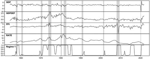
We consider the quarterly U.S. data covering the period from 1954Q3 to 2021Q4 (270 observations) and consisting of four variables: real GDP (GDP), GDP implicit price deflator (GDPDEF), producer price index (all commodities, PPI), and an interest rate variable (RATE). We detrend the former three by taking the first-differences and multiplying by hundred, so the resulting series approximate the percentage growth rates. Our policy variable is the interest rate variable, which is the effective federal funds (FF) rate from 1954Q3 to 2008Q2. After that we replace it with the Wu and Xia (2016) shadow rate, which is not restricted by the zero lower bound and also quantifies unconventional monetary policy measures. The Wu and Xia (2016) shadow rate series was retrieved from the Federal Reserve Bank of Atlanta’s website and the rest of the data were retrieved from the Federal Reserve Bank of St. Louis database. The series are presented in the first four top panels of Figure 1 with the shaded areas indicating the periods of the NBER based U.S. recessions.

Figure 1: Quarterly U.S. series covering the period from 1954Q3 to 2021Q4. From the top to the bottom, the first three panels present the log-differences of real GDP (GDP), GDP implicit price deflator (GDPDEF), and producer price index (PPI) multiplied by hundred. The fourth panel presents an interest rate variable, which is the effective federal funds from 1954Q3 to 2008Q2 and the Wu and Xia (2016) shadow rate from 2008Q3 to 2021Q4. The bottom panel shows the estimated mixing weights of the first regime of the fitted VAR $p=4$ model with two volatility-regimes. The shaded areas indicate the NBER based U.S. recessions.

We select the order of the SVAR model by first finding a suitable autoregressive order for a linear Gaussian VAR. The AIC is minimized by the order $p=3$ (with the value 9.185), suggesting that this might be the appropriate lag order for modeling autocorrelation. The diagnostics presented in an online appendix show that the residuals of the linear VAR model are clearly heteroscedastic. Therefore, we add a second volatility regime and estimate a two-regime VAR model with $p=3$, which obtains the AIC 7.531 superior to the linear model. The (adjusted) Portmanteau test for remaining autocorrelation in the residuals taking into account 20 lags rejects the adequacy of the two-regime $p=3$ model at the $5\%$ level of significance (p-value 0.038). Hence, we increase the autoregressive order of our model to $p=4$, which obtains the AIC 7.650. Our two-regime $p=4$ model passes the Portmanteau test at the $5\%$ level of significance (p-value 0.065), so it is preferred over the $p=3$ model despite of the larger AIC.

In our view, the adequacy of the two-regime $p=4$ model is decent enough for further analysis, but there is some conditional heteroscedasticity remaining in the (quantile) residuals. Hence, adding a third volatility regime to the model is considered. The three-regime model obtains a smaller AIC (7.129) than the two-regime model, but some heteroscedasticity still remains in the (quantile) residuals. The adequacy of the three-regime model is, nevertheless, rejected by the Portmanteau test for remaining autocorrelation (p-value 0.0005). Since the three-regime model also induces a long-run price puzzle to the IRFs, the more parsimonious two-regime model is preferred as the main specification. Details on the model selection and diagnostics are given in an online appendix.

The bottom panel of Figure 1 displays the estimated mixing weights for the first volatility regime of the fitted two-regime VAR $p=4$ model. The first regime prevails in the late 1950s, in the 1970s and 1980s, during the Financial crisis, in 2015 and 2016, and finally during the COVID-19 crisis from the third quarter of 2020 onwards. Conversely, the second regime dominates when the first regime does not. The first regime thereby seems to mainly accommodate more volatile periods than the second regime.

5.1 Identification of the Monetary Policy Shock

Decomposing the covariance matrices of the reduced form VAR $p=4$ model with two-volatility regimes as in (3.4) gives the following estimates for the structural parameters: (5.1) $$\begin{array}{c}\widehat{W}=\left[\begin{array}{cccc}0.24(0.376)& -\mathbf{0}.\mathbf{59}(0.226)& \mathbf{1}.\mathbf{58}(0.188)& -0.42(0.427)\\ -\mathbf{0}.\mathbf{27}(0.085)& 0.13(0.194)& \mathbf{0}.\mathbf{21}(0.054)& -0.06(0.069)\\ 0.35(1.068)& \mathbf{1}.\mathbf{68}(0.312)& \mathbf{1}.\mathbf{38}(0.339)& -0.59(0.444)\\ 0.05(0.077)& 0.06(0.079)& \mathbf{0}.\mathbf{57}(0.204)& \mathbf{1}.\mathbf{18}(0.180)\end{array}\right],\hfill \\ {\widehat{\lambda }}_2=\left[\begin{array}{c}\mathbf{0}.\mathbf{35}(0.076)\\ \mathbf{0}.\mathbf{28}(0.053)\\ \mathbf{0}.\mathbf{10}(0.018)\\ \mathbf{0}.\mathbf{05}(0.010)\end{array}\right],\hfill \end{array}$$(5.1) where the ordering of the variables is $y_t=({\text{GDP}}_t,{\text{GDPDEF}}_t,{\text{PPI}}_t,{\text{RATE}}_t)$, the estimates ${\widehat{\lambda }}_{2i}$ are in a decreasing order (which fixes the ordering of the columns of $\widehat{W}$), the last element of each column is normalized to be positive, and approximate standard errors are given in parentheses next to the estimates. The estimates that deviate from zero by more than two times their approximate standard error are bolded.

Based on the estimates and their standard errors in (5.1), only the third and fourth shock move the interest variable significantly at impact. The third shock moves production and both prices significantly to the same direction as the interest rate variable, so its characteristics appear similar to an aggregate demand shock and not a monetary policy shock. The last shock, in contrast, moves GDP, inflation, and commodity price inflation to the opposite direction from the interest rate variable, which is consistent with standard economic theory (e.g., Galí 2015, and the references therein). Since the characteristics of the last shock mostly resemble those of a monetary policy shock, we deem it as the monetary policy shock.

If Assumption 1 holds, the shocks are statistically identified. Considering the estimates of ${\lambda }_{2i}$, $i=1,2,3,4$, and their standard errors, there does not seem to be any particular reason to believe that ${\lambda }_{24}$ (corresponding to the last shock) could be identical to any of ${\lambda }_{2i}$, $i=1,2,3$. On the other hand, the estimates of ${\lambda }_{21}$ and ${\lambda }_{22}$ are relatively close to each other. It is, nonetheless, difficult to formally justify that ${\lambda }_{2i}$, $i=1,2,3,4$, are different to each other, as the standard errors of their estimates are valid only if the assumption holds in the first place (see also the related discussion in Section 3.2). If the validity of Assumption 1 is a concern, note that by Proposition 2, the monetary policy shock is still identified if ${\lambda }_{2i}={\lambda }_{2j}$ for any $i,j=1,2,3$, as long as ${\lambda }_{2i}\ne {\lambda }_{24}$ for $i=1,2,3$ (Condition 2 of Proposition 2). Condition 2 of Proposition 2, in turn, is satisfied by the estimated impact responses in (5.1), because the monetary policy shock is the only shock that moves the interest rate variable to the opposite direction from all the other variables at impact.

The identification can also be strengthened by placing a zero restriction, for instance, on the instantaneous effect of inflation to the monetary policy shock. In this case, the monetary policy shock is identified by Proposition 3 also when ${\lambda }_{23}={\lambda }_{24}$, assuming that the instantaneous response of inflation to the third shock is not zero. Imposing the zero restriction on the impact response of the inflation does not change the estimated impulse response functions much, but it induces a slight short-term price puzzle (see Section 5.3).

5.2 Impulse Response Functions

Figure 2 presents the IRFs $h=0,1,\dots ,32$ quarters ahead estimated for a contractionary one-standard-error monetary policy shock (solid line) and bootstrapped $90\%$ confidence bounds based on 2500 replications (dashed lines). The IRFs of the GPD growth rate, inflation rate and commodity price inflation rate are accumulated to ($100\times$)log levels. The GDP decreases significantly in response to a contractionary monetary policy shock. The IRF has a persistent hump-shaped pattern with the peak response occurring after six quarters. Then, the response starts to slowly return toward zero and settles to a small permanent decrease in the point estimate.

Figure 2: Impulse response functions $h=0,1,\dots ,32$ quarters ahead for a one-standard-error monetary policy shock. The IRFs of the GDP (top left), GDP deflator (bottom left), and producer price index (top right) are accumulated to log-levels. The IRF of the interest rate variable is presented in the bottom right figure. Point estimates are presented with solid line and bootstrapped $90\%$ confidence bounds (based on 2500 replications) are presented with dashed lines.

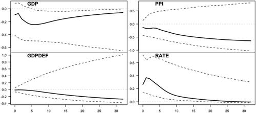
The prices (including producer prices) decrease permanently in response to a contractionary monetary policy shock. Notably, there is no price puzzle, but the decrease of the GDP deflator is very small for roughly a year after the impact, before it starts to decrease more substantially. Our results are, therefore, consistent with the cost-channel of monetary policy potentially causing short-run inertia in the response of prices (see, e.g., Barth and Ramey 2001; Christiano, Eichenbaum, and Evans 2005). The bootstrapped confidence bounds of the responses of the prices are very wide, however. Lastly, the response of the interest variable increases at first and then slowly decays toward zero.

Overall, our findings are in line with much of the related literature in that the response of output is significant, but our results lack the frequently reported price puzzle (see, e.g., Ramey 2016, chap. 3, and the references therein). The immediate decrease in output and a slow response of prices aligns with Lanne, Meitz, and Saikkonen (2017), who identify the monetary policy shock by non-Gaussianity. Herwartz and Lütkepohl (2014), however, present contrasting results. They report a short-run increase in output and a more significant immediate decrease in the price level in response to a contractionary monetary policy shock identified by heteroscedasticity.

5.3 Robustness Checks

As robustness checks, several alternative specifications are considered. The main results are summarized here, and further details are provided in an online appendix. In particular, the IRFs obtained for the alternative specifications are presented in Figure 6 of the online appendix. For comparison, we consider the standard recursively identified linear Gaussian SVAR model with the monetary policy shock ordered last. This model not only displays a medium-run price puzzle but also a short-run output puzzle, that is, the response of GDP to a contractionary shock is positive in the point estimate for a short period of time before becoming negative.

To investigate the sensitivity of our results to the choice of p in our SVAR model with two volatility regimes, we estimate the IRFs for the model with the autoregressive order $p=3$. The IRFs are very similar to our benchmark specification, but the response of the GDP deflator is slightly positive from the second to the fourth quarter after the impact. To study how sensitive our findings are to the number of volatility regimes, we fit a SVAR model with three volatility regimes ($M=3$). The IRFs display a significant decrease in output but also a long-run price puzzle.

We also consider strengthening our identification by placing a zero restriction on the instantaneous response of the GDP deflator to the monetary policy shock. We find the IRFs quite similar to our benchmark specification with the exception that the zero restriction seems to induce a slight short-term price puzzle. To check whether our results are robust to excluding the COVID-19 period, we fit our two-regime SVAR model to the sub-sample that ends 2019Q4. The IRFs turn out to be otherwise rather similar to the benchmark specification except that there is a short-term price puzzle.

In order to see how robust the results are to using alternative methods for detrending the log of the GDP, we consider the backward-looking Hodrick-Prescott (HP) filter and the linear projection filter proposed by Hamilton (2018). In both of these specifications, there is a severe long-run price puzzle. The specification employing the linear projection filter also displays a severe production puzzle, as the GDP increases in response to a supposedly contractionary monetary policy shock. With the HP filter, the response of the GDP is negative and hump-shaped but relatively short-lived.

Overall and in line with Ramey (2016, chap. 3), the significant decrease of output in response to a contractionary monetary policy shock seems quite robust across the considered specifications. The specification employing the linear projection filter proposed by Hamilton (2018) is an exception, however. Many of the specifications produce a price puzzle, with its severity varying substantially.

Finally, it is useful to study whether the monetary policy shock behaves consistently to its real history in particular points of time, such as the Volcker recession in the early 1980s. Since our model assumes linear autoregressive dynamics, the reduced form errors and thereby also structural shocks can be recovered from the fitted model (it may, hence, be also possible to make use of historical-narrative restrictions in identification). Prior to the Volcker recession in 1979Q3 and 1979Q4, the identified monetary policy shock implied by our model turns out to be contractionary and medium to large sized. We found that during the interest rate cuts in 1980, the monetary policy shocks were expansionary, and thereafter the vast interest rate increase was accompanied by a large contractionary monetary policy shock.

6 Summary

We have introduced a structural vector autoregressive model with regime-switching in the conditional covariance matrix. The switching probabilities are determined endogenously through the full distribution of the preceding p observations. The reduced form model is obtained with parameter restrictions from the GMVAR model of Kalliovirta, Meitz, and Saikkonen (2016) by assuming time-invariant intercepts and autoregressive matrices. The structural shocks are identified by simultaneously diagonalizing the reduced form error covariance matrices, which restricts the effects of the shocks identical across the volatility regimes.

In line with the statistical identification literature, our model generally identifies the structural shocks up to ordering and sign, but additional information is needed to label the identified shocks, or to give them an economic interpretation. Due to identification, it is possible to test for economic restrictions to label the shocks. Since it is not always clear whether the assumption that is required for statistical identification is satisfied, and its validity difficult to justify formally, we made use of the matrix decomposition proposed by Lanne and Lütkepohl (2010) and Lanne, Lütkepohl, and Maciejowska (2010) to derive general conditions for identifying a subset of the shocks when this assumption fails. The article is accompanied with the CRAN distributed R package gmvarkit (Virolainen 2018a), which provides a comprehensive set of tools for numerical analysis of the model.

To illustrate the use of our methods, we studied the effects of the monetary policy shock in an empirical application to the U.S. quarterly data. The monetary policy shock was identified as the only shock that moves the interest rate variable to the opposite direction from output and prices at impact. We found that a contractionary monetary policy shock significantly decreases output in a persistent hump-shaped pattern. Prices decrease permanently, and while there is no price puzzle in the point estimate, we found short-run inertia in the response of prices.

One potential area of future research is applying the identification method of Bacchiocchi and Fanelli (2015) and Angelini et al. (2019) to the our SVAR model. This approach would relax the assumption of constant relative impact responses across the volatility regimes, but it requires imposing untestable zero restrictions on the impact matrices. Additionally, to address the selection of the number of regimes in our model, it might be useful to generalize the test of Meitz and Saikkonen (2021) that tests for the number regimes in the univariate counterpart of the GMVAR model, to the multivariate case.

Supplementary Materials

The supplementary material includes a pdf file that contains the online appendices. The online appendices provide proofs for the states lemma and propositions, a Monte Carlo study on finite sample performance of the maximum likelihood estimator, and details on the empirical application.

Acknowledgments

The author thanks Markku Lanne, Mika Meitz, and Pentti Saikkonen who helped to improve this article substantially. The author also thanks Atsushi Inoue (the editor), the two anonymous referees as well as Henri Nyberg and Antti Ripatti for the useful comments.

Disclosure Statement

The author has no conflict of interest to declare.

Additional information

Funding

This work was supported by the Academy of Finland under Grants 308628 and 347986.

References

- Angelini, G., Bacchiocchi, E., Caggiano, G., and Fanelli, L. (2019), “Uncertainty Across Volatility Regimes,” Journal of Applied Econometrics, 34, 437–455. DOI: 10.1002/jae.2672.
- Bacchiocchi, E., and Fanelli, L. (2015), “Identification in Structural Vector Autoregressive Models with Structural Changes, with an Application to US Monetary policy,” Oxford Bulletin of Economics and Statistics, 77, 761–779. DOI: 10.1111/obes.12092.
- Barth, M. J., and Ramey, V. A. (2001), “The Cost Channel of Monetary Transmission,” in NBER Macroeconomics Annual, eds. B. S. Bernanke and K. Rogoff (Vol. 16), pp. 199–239, Cambridge, MA: MIT Press. DOI: 10.1086/654443.
- Christiano, L. J., Eichenbaum, M., and Evans, C. L. (2005), “Nominal Rigidities and the Dynamic Effects of a Shock to Monetary Policy,” Journal of Political Economy, 113, 1–45. DOI: 10.1086/426038.
- Galí, J. (2015), Monetary Policy, Inflation, and the Business Cycle (2nd ed.), Princeton and Oxford: Princeton University Press.
- Hamilton, J. D. (2018), “Why You Should Never Use the Hodrick-Prescott Filter,” The Review of Economics and Statistics, 100, 831–843. DOI: 10.1162/rest_a_00706.
- Herwartz, H., and Lütkepohl, H. (2014), “Structural Vector Autoregressions with Markov Switching: Combining Conventional with Statistical Identification of Shocks,” Journal of Econometrics, 183, 104–116. DOI: 10.1016/j.jeconom.2014.06.012.
- Kalliovirta, L., Meitz, M., and Saikkonen, P. (2015), “A Gaussian Mixture Autoregressive Model for Univariate Time Series,” Journal of Time Series Analysis, 36, 247–266. DOI: 10.1111/jtsa.12108.
- ——— (2016), “Gaussian Mixture Vector Autoregression,” Journal of Econometrics, 192, 465–498.
- Kalliovirta, L., and Saikkonen, P. (2010), “Reliable Residuals for Multivariate Nonlinear Time Series Models,” Unpublished revision of HECER discussion paper No. 247.
- Kilian, L., and Lütkepohl, H. (2017), Structural Vector Autoregressive Analysis (1st ed.), Cambridge: Cambridge University Press.
- Lanne, M., and Lütkepohl, H. (2010), “Structural Vector Autoregressions With Nonnormal Residuals,” Journal of Business & Economic Statistics, 28, 159–168. DOI: 10.1198/jbes.2009.06003.
- Lanne, M., Lütkepohl, H., and Maciejowska, K. (2010), “Structural Vector Autoregressions with Markov Switching,” Journal of Economic Dynamics and Control, 34, 121–131. DOI: 10.1016/j.jedc.2009.08.002.
- Lanne, M., Meitz, M., and Saikkonen, P. (2017), “Identification and Estimation of Non-Gaussian Structural Vector Autoregressions,” Journal of Econometrics, 196, 288–304. DOI: 10.1016/j.jeconom.2016.06.002.
- Lewis, D. (2021), enquoteIdentifying Shocks via Time-Varying Volatility, The Review of Economic Studies, 88, 3086–3124. DOI: 10.1093/restud/rdab009.
- Lütkepohl, H. (2005), New Introduction to Multiple Time Series Analysis (1st ed.), Berlin: Springer.
- Lütkepohl, H., Meitz, M., Netšunajev, A., and Saikkonen, P. (2021), “Testing Identification via Heteroskedasticity in Structural Vector Autoregressive Models,” The Econometrics Journal, 24, 1–22. DOI: 10.1093/ectj/utaa008.
- Lütkepohl, H., and Netšunajev, A. (2014), “Disentangling Demand and Supply Shocks in the Crude Oil Market: How to Check Sign Restrictions in Structural VARs,” Journal of Applied Econometrics, 29, 479–496. DOI: 10.1002/jae.2330.
- ——— (2017), “Structural Vector Autoregressions with Smooth Transitions in Variances,” Journal of Economic Dynamics & Control, 84, 43–57.
- Lütkepohl, H., and Schlaak, T. (2018), “Choosing Between Different Time-Varying Volatility Models for Structural Vector Autoregressive Analysis,” Oxford Bulletin of Economics and Statistics, 80, 715–735. DOI: 10.1111/obes.12238.
- Meitz M., Preve D., Saikkonen P. (2023), “A Mixture Autoregressive Model based on Student’s t-distribution,” Communications in Statistics - Theory and Methods, 52, 499–515. DOI: 10.1080/03610926.2021.1916531.
- Meitz, M., and Saikkonen, P. (2021), “Testing for Observation-Dependent Regime Switching in Mixture Autoregressive Models,” Journal of Econometrics, 222, 601–624. DOI: 10.1016/j.jeconom.2020.04.048.
- Muirhead, R. (1982), Aspects of Multivariate Statistical Theory (1st ed.), Hoboken, NJ: Wiley.
- Netsunajev, A. (2013), “Reaction to Technology Shocks in Markov-Switching Structural VARs: Identification via Heteroskedasticity,” Journal of Macroeconomics, 36, 51–62. DOI: 10.1016/j.jmacro.2012.12.005.
- Normandin, M., and Phaneuf, L. (2004), “Monetary Policy Shocks: Testing Identification Conditions under Time-Varying Conditional Volatility,” Journal of Monetary Economics, 51, 1217–1243. DOI: 10.1016/S0304-3932(04)00069-8.
- Ramey, V. A. (2016), “Macroeconomic Shocks and Their Propagation,” in Handbook of Macroeconomics (Vol. 2), eds. J. B. Taylor and H. Uhlig, Amsterdam: Elsevier Science B.V.
- Rigobon, R. (2003), “Identification through Heteroskedasticity,” The Review of Economics and Statistics, 85, 777–792. DOI: 10.1162/003465303772815727.
- Virolainen, S. (2018a), gmvarkit: Estimate Gaussian and Student’s t Mixture Vector Autoregressive Models, R package version 2.1.0 available at CRAN: https://CRAN.R-project.org/package=gmvarkit.
- ——— (2018b), uGMAR: Estimate Univariate Gaussian and Student’s t Mixture Autoregressive Models, R package version 3.4.2 available at CRAN: https://CRAN.R-project.org/package=uGMAR.
- ——— (2022), “A Mixture Autoregressive Model based on Gaussian and Student’s t-distributions,” Studies in Nonlinear Dynamics & Econometrics, 26, 559–580.
- Wu, J., and Xia, F. (2016), “Measuring the Macroeconomic Impact of Monetary Policy at the Zero Lower Bound,” Journal of Money, Credit and Banking, 48, 253–291. DOI: 10.1111/jmcb.12300.