Grouped Heterogeneity in Linear Panel Data Models with Heterogeneous Error Variances

Abstract

We develop a procedure to identify latent group structures in linear panel data models that exploits a grouping in the error variances of cross-sectional units. To accommodate such grouping, we introduce an objective function that avoids a singularity that arises in a pseudolikelihood approach. We provide theoretical and numerical evidence showing when allowing for variance groups improves classification. The developed procedure provides new evidence on the relation between firm-level research and development (R&D) investments and the business cycle. We find a well-defined group structure in the variances that ex-post can be related to firm size. Our estimates indicate stronger procyclical investment patterns at medium-size firms compared to large firms.

Keywords:

• Clustering
• Panel data
• R&D investment

1 Introduction

Panel datasets are widely used to control for unobserved heterogeneity via the inclusion of fixed effects. Modeling more flexible patterns of heterogeneity is challenging as the number of parameters quickly proliferates. A parsimonious approach is to cluster similar units into a small number of latent groups. Bonhomme and Manresa (2015) introduce the grouped fixed-effects (GFE) estimator that uncovers these groups by capitalizing on separation in the slope coefficients and time effects across groups, which we will refer to as separation in the means. Recent extensions allow for nonlinear models (Liu et al. 2020), threshold models (Miao, Su, and Wang 2020), heterogeneous structural breaks (Okui and Wang 2021), and breaks in group membership (Lumsdaine, Okui, and Wang 2023). A necessary condition for GFE to consistently classify the cross-sectional units is that the separation in the means is sufficiently strong. In this article, we consider the question whether it is possible to achieve consistent classification when the means are possibly weakly separated, but there is information on the grouping available from the error variances. This is motivated by our study of the relation between R&D investments and the business cycle. There is mixed evidence on the heterogeneity of this relation across firms, indicating that the separation in the means is weak. However, theory suggests that the cyclicality of R&D investments relates to “firm size”: large firms smooth R&D investments, which not only dampens the correlation with the business cycle but also lowers the variance of investments. The information from the variances then allows us to uncover the group structure. By estimating the grouping from the data, we also avoid relying on one particular “firm size” measure.

There are two main challenges in allowing for grouping in the error variances. First, to attain consistent classification when the means are weakly separated, we necessarily need to assume that there is information on the mean grouping in the variances. However, when the means are strongly separated, the information we use from the variances should be limited and the performance of the developed algorithm should approach that of GFE, which makes no assumptions on the variance heterogeneity. Second, GFE can be interpreted as the maximizer of the pseudolikelihood for a Gaussian mixture model where the error variances do not differ between groups. When we extend this argument to allow for group-specific variances, the presence of grouped time effects induces a singularity in the pseudolikelihood. As a consequence, the global minimum of the objective function does not exist.

We address these challenges by deviating from the pseudolikelihood perspective. Instead we consider a square root objective function that shares some crucial features with the pseudolikelihood. Conditional on the grouping, both functions are minimized by the same estimators for the slope coefficients, grouped time fixed effects and error variances. However, we show that the square root objective function is more sensitive to the grouping in the means relative to the pseudolikelihood approach. As a result, both the estimators obtained from the square root objective function (GSR) as the pseudolikelihood (GPL) improve over GFE when there is a group structure in the variances, but only GSR offers numerically similar results to GFE under strong mean separation and no group structure in the variances. Finally, the square root objective function does not include the logarithmic term that causes the aforementioned singularities in the pseudolikelihood approach.

We show consistency of the GSR estimator for the parameters as well as consistency of the group assignment when the number of units N and the number of time periods T tend to infinity simultaneously. The asymptotic results show that if there is group-level variance heterogeneity, GSR achieves consistent classification even when the separation in slope coefficients and grouped-fixed effects is small.

To illustrate the proposed method, we consider two empirical applications. First, we consider the relation between R&D investment and the business cycle. Empirically, it is found that for most firms the relation between investment and output is procyclical (Barlevy 2007; Fabrizio and Tsolmon 2014; van Ophem et al. 2019). There is evidence that this relation is heterogeneous across firms, but the drivers for this heterogeneity are not obvious. Fabrizio and Tsolmon (2014) argue for a role of obsolescence, while van Ophem et al. (2019) point to external financing. The somewhat ambiguous results suggest that separation in the mean is likely small and difficult to detect. However, the variance of investment is expected to differ substantially across firms. For example, large firms can better smooth investment over time and hence tend to have lower variance in investment growth rates (Bachmann and Bayer 2014). We can use such separation in terms of the variance to identify differences in cyclicality of investment patterns across firms.

We indeed find a well-defined group structure when allowing for variance groups. Ex-post the groups can be related to firm size: the low-variance group is associated with large firms, while the high-variance group is composed of small firms. We document substantial variation in cyclicality of R&D investments across the identified groups. When we estimate the model with three latent groups and control for firm balance-sheet characteristics, we find a medium-variance group that is highly procyclical, and a low-variance group that is less procyclical. This aligns with findings by Crouzet and Mehrotra (2020), who show that large firms are less cyclically sensitive compared to smaller firms. In addition, we also find a high-variance group with acyclical behavior. A dedicated Monte Carlo further corroborates that taking into account variance differences results in more accurate estimation of group memberships and model parameters. Importantly, this result continues to hold if there is heterogeneity in the time averaged variances within groups.

In the second empirical application, we analyze whether GSR performs well relative to GFE when the separation in the means is strong. We revisit the relation between income and democracy studied by Bonhomme and Manresa (2015). A Monte Carlo simulation dedicated to this setting shows that the classification accuracy based on GSR is similar to that of GFE even when the variances do not exhibit a grouping structure. Without a grouping structure in the variance, the pseudolikelihood objective function suffers a considerable decrease in its classification accuracy, which highlights that this objective function assigns more weight to the variances relative to the square root objective function. Empirically, our results confirm the income effects estimated by Bonhomme and Manresa (2015).

Related literature

There are various methods to identify and estimate latent groups in panel datasets. One strand of the literature focuses on various adaptations of k-means clustering (Lin and Ng 2012; Sarafidis and Weber 2015; Bonhomme and Manresa 2015; Ando and Bai 2017; Bonhomme, Lamadon, and Manresa 2022) that results in an iterative process between the estimation of the group membership and the estimation of the model parameters. An alternative is to consider the lasso approach (Su, Shi, and Phillips 2016; Lu and Su 2017; Wang, Phillips, and Su 2018), where the group membership and the model parameters are estimated simultaneously. Our article is closely related to the first strand. However, while our objective function can be related to the square root lasso by Belloni, Chernozhukov, and Wang (2011), it does not include a penalty term.

Allowing for group-specific variance is common in the application of dynamic mixture models in macroeconomics, where negative GNP growth tends to go hand in hand with high variance (Carrasco, Hu, and Ploberger 2014), or in finance, where negative asset returns are accompanied by high volatility (Hamilton and Lin 1996). The emergence of singularities is a well-known phenomenon in these more flexible mixture models. One proposed solution is to select an appropriate local maximizer. Kiefer (1978) shows that there exists a local maximizer that is consistent and asymptotically efficient. However, several local maximizers can exist for a given sample, and it is difficult to determine when the best one has been found. To circumvent this problem, Hathaway (1985) proposes to maximize a restricted log-likelihood that imposes a lower bound on the variances, while Hamilton (1991) proposes a quasi-Bayesian approach. These approaches require either the selection of a variance threshold parameter or the specification of an appropriate prior distribution. Specific applications of mixture models in panel data settings have been considered by Sun (2005), Kasahara and Shimotsu (2009), and Browning and Carro (2010). Estimation of these models generally relies on an expectation-maximization algorithm that estimates group membership probabilities, rather than the hard group assignment that we use.

As an alternative to modeling heterogeneity in the mean and variance, one could consider a fully distributional approach based on a quantile regression framework (Zhang, Wang, and Zhu 2019; Gu and Volgushev 2019; Leng, Chen, and Wang 2023). This approach is substantially more flexible than separation in slope or variance coefficients. However, it does require that the separation in the slope coefficients for at least one quantile is sufficiently large, for example Assumption 1(v) in Leng, Chen, and Wang (2023). The method we consider in this article does not impose a lower bound on the magnitude of the difference in the means, as long as the error variances contain information about the group structure.

Finally, we assume that the slope coefficients and time fixed effects are the same within groups. Recently, Bonhomme, Lamadon, and Manresa (2022) analyze how continuous heterogeneity can be approximated by discrete groups. The approach considered there is to group based on observed moments of the data, and possibly apply the original k-means grouping algorithm in a second stage. When the second moment is arguably important, our proposed method can therefore complement the approach of Bonhomme, Lamadon, and Manresa (2022) by replacing the k-means objective function with the square root objective function. We leave this extension to further research.

Outline

In Section 2, we introduce the model and the square root objective function, and we discuss the estimation procedure. In Section 3, we provide theoretical results. Proofs and technical details are provided in the supplementary material. Section 4 discusses two empirical applications with dedicated Monte Carlo simulations. Section 5 concludes.

2 Model and Estimation

We consider the following linear panel data model, (1) $$\begin{array}{cc}{y}_{\mathit{\text{it}}}\hfill & ={\mathit{x}}_{\mathit{\text{it}}}^{\prime }{\mathit{\theta }}_{g_i}+{\alpha }_{g_{i}t}+v_{\mathit{\text{it}}},\hspace{1em}i=1,\dots ,N,\hspace{1em}t=1,\dots ,T,\hfill \end{array}$$(1) where $g_i\in \{1,\dots ,G\}$ indicates the group label for unit i. For each group g, we have different slope coefficients ${\mathit{\theta }}_g$ and time-effects α_gt . Alternatively, we could write ${\mathit{\theta }}_{g_i}={\sum }_{g=1}^{G}1[g_i=g]{\mathit{\theta }}_g$ and ${\alpha }_{g_{i}t}={\sum }_{g=1}^{G}1[g_i=g]{\alpha }_{\mathit{\text{gt}}}$, where $1[g_i=g]$ is an indicator function that indicates the group membership of unit i. Equation (1)(1) $$\begin{array}{cc}{y}_{\mathit{\text{it}}}\hfill & ={\mathit{x}}_{\mathit{\text{it}}}^{\prime }{\mathit{\theta }}_{g_i}+{\alpha }_{g_{i}t}+v_{\mathit{\text{it}}},\hspace{1em}i=1,\dots ,N,\hspace{1em}t=1,\dots ,T,\hfill \end{array}$$(1) covers different specifications such as a model with time-invariant fixed effects (${\alpha }_{g_{i}t}={\alpha }_i$), a model with constant slope coefficients across individuals (${\mathit{\theta }}_{g_i}=\mathit{\theta }$), or an intermediate case where a subset of slope coefficients is constant across groups.

The present article assumes that the unconditional variance of v_it in (1) is group-specific. In particular, if the group index of the ith unit $g_i=g$, then we define (2) $${\sigma }_g^2=\underset{(N,T)\to \infty }{\mathrm{\text{lim}}}\frac{\sum _{i=1}^N\sum _{t=1}^{T}1[g_i=g]\mathbb{E}\left[v_{\mathit{\text{it}}}^2\right]}{T\sum _{i=1}^{N}1[g_i=g]}.$$(2)

Differences in ${\sigma }_g^2$ across groups can then be used to identify group memberships.

2.1 Estimation

We gather the unknown parameters in $(\mathit{\theta },{\mathit{\sigma }}^2,\mathit{\alpha },\mathit{\gamma })$. The group-specific time effects ${\alpha }_{\mathit{\text{gt}}}\in \mathcal{A}\subset \mathbb{R}$ for $g=1,\dots ,G$ and $t=1,\dots ,T$, and we denote by $\mathit{\alpha }$ the set of all α_gt ’s. The slope coefficients ${\mathit{\theta }}_g\in \mathbf{\Theta }\subset {\mathbb{R}}^K$ for $g\in \{1,\dots ,G\}$ and $\mathit{\theta }=({\mathit{\theta }}_1^{\prime },\dots ,{\mathit{\theta }}_G^{\prime })\prime$. The variance of the groups ${\sigma }_g^2\in \Xi \subset {\mathbb{R}}^{+}$ for $g\in \{1,\dots ,G\}$ and ${\mathit{\sigma }}^2=({\sigma }_1^2,\dots ,{\sigma }_G^2)\prime$. The group membership vector $\mathit{\gamma }=(g_1,\dots ,g_N)\prime \in {\mathbf{\Gamma }}_G$ that is $N\times 1$, where ${\mathbf{\Gamma }}_G$ denotes the set of all possible groupings into at most G groups.

Bonhomme and Manresa (2015) simultaneously estimate the slope coefficients ${\mathit{\theta }}_{g_i}$, the grouped time effects ${\alpha }_{g_{i}t}$, and the grouping $\mathit{\gamma }$ by minimizing the objective function (3) $$\begin{array}{cc}Q(\mathit{\theta },\mathit{\alpha },\mathit{\gamma })\hfill & =\frac{1}{\mathit{\text{NT}}}\sum _{i=1}^N\sum _{t=1}^T{(y_{\mathit{\text{it}}}-{\mathit{x}}_{\mathit{\text{it}}}^{\prime }{\mathit{\theta }}_{g_i}-{\alpha }_{g_{i}t})}^2,\hfill \end{array}$$(3) over $(\mathit{\theta },\mathit{\alpha },\mathit{\gamma })\in {\mathbf{\Theta }}^G\times {\mathcal{A}}^{\mathit{\text{GT}}}\times {\Gamma }_G$. Restricting ${\mathit{\theta }}_{g_i}=\mathit{\theta }$ yields the grouped fixed effects estimator (GFE).

In order to exploit group-level variance heterogeneity, we extend (3) to (4) $$\begin{array}{cc}\hfill & Q(\mathit{\theta },{\mathit{\sigma }}^2,\mathit{\alpha },\mathit{\gamma })=\frac{1}{\mathit{\text{NT}}}\sum _{i=1}^N\sum {}_{t=1}^T\hfill \\ \hfill & \mathrm{\hspace{1em}}\mathrm{\hspace{1em}}\left[h_{m,1}({\sigma }_{g_i}^2)+h_{m,2}({\sigma }_{g_i}^2){\left(y_{\mathit{\text{it}}}-{\mathit{x}}_{\mathit{\text{it}}}^{\prime }{\mathit{\theta }}_{g_i}-{\alpha }_{g_{i}t}\right)}^2\right],\hfill \end{array}$$(4) which is minimized over $(\mathit{\theta },{\mathit{\sigma }}^2,\mathit{\alpha },\mathit{\gamma })\in {\mathbf{\Theta }}^G\times {\Xi }^G\times {\mathcal{A}}^{\mathit{\text{GT}}}\times {\Gamma }_G$. Two possible choices for the pair of functions $(h_{m,1}(x),h_{m,2}(x))$ are (5) $$\text{Grouped pseudolikelihood }(\text{GPL}):{\mathrm{h}}_{1,1}(\mathrm{x})\text{=}\hspace{0.17em}\mathrm{\text{log}}\hspace{0.17em}(\mathrm{x}),\hspace{1em}{\mathrm{h}}_{1,2}(\mathrm{x}){\text{=x}}^{-1},$$(5) (6) $$\text{Grouped Square Root }(\text{GSR}):{\mathrm{h}}_{2,1}(\mathrm{x}){\text{=x}}^{\text{1/2}},\hspace{1em}{\mathrm{h}}_{2,2}(\mathrm{x}){\text{=x}}^{-1/2}.$$(6)

The choice (5) results from extending the Gaussian pseudolikelihood to the case where the error variance is group-specific. This extension has intuitive appeal; however, in the presence of grouped fixed effects, it is possible to obtain a perfect fit for individual i if that individual is the sole member of group g. The error variance for this particular group is estimated as ${\widehat{\sigma }}_g^2=0$, and the logarithm appearing in (5) yields minus infinity. This shows that a global minimizer does not exist, and the minimization procedure breaks down. We provide numerical evidence for this problem in the supplementary material, which shows that the number of runs of an algorithm that results in a singularity increases with the number of groups.

The singularity problem in (5) is resolved by the objective function resulting from (6), which no longer contains the logarithmic term. We refer to this objective function as the Grouped Square Root (GSR) objective function since it resembles the square root lasso (Belloni, Chernozhukov, and Wang 2011; Sun and Zhang 2012) without the inclusion of an l₁ penalty term. We refer to the estimators resulting from the minimization of problem (4) combined with (6) as the GSR estimators.

An attractive feature of (6) is that conditional on a grouping $\mathit{\gamma }$, the estimators for the slope coefficients, group fixed effects, and variance take their usual form. The objective function (4) is minimized through alternating minimization steps. First, conditional on a grouping $\mathit{\gamma }$, we estimate ${\mathit{\theta }}_g$, α_gt , and ${\sigma }_{\mathit{\text{gt}}}^2$. The estimators that minimize $Q(\mathit{\theta },{\mathit{\sigma }}^2,\mathit{\alpha },\mathit{\gamma })$ are (7) $${\widehat{\mathit{\theta }}}_g={\left(\sum _{i=1}^N\sum _{t=1}^{T}1[g_i=g]{\tilde{\mathit{x}}}_{\mathit{\text{it}},g}{\tilde{\mathit{x}}}_{\mathit{\text{it}},g}^{\prime }\right)}^{-1}\sum _{i=1}^N\sum _{t=1}^{T}1[g_i=g]{\tilde{\mathit{x}}}_{\mathit{\text{it}},g}{\tilde{y}}_{\mathit{\text{it}},g},$$(7) (8) $${\widehat{\alpha }}_{\mathit{\text{gt}}}=\frac{\sum _{i=1}^{N}1[g_i=g](y_{\mathit{\text{it}}}-{\mathit{x}}_{\mathit{\text{it}}}^{\prime }{\widehat{\mathit{\theta }}}_g)}{\sum _{i=1}^{N}1[g_i=g]},$$(8) (9) $${\widehat{\sigma }}_g^2=\frac{\sum _{t=1}^T\sum _{i=1}^{N}1[g_i=g]{(y_{\mathit{\text{it}}}-{\mathit{x}}_{\mathit{\text{it}}}^{\prime }{\widehat{\mathit{\theta }}}_g-{\widehat{\alpha }}_{\mathit{\text{gt}}})}^2}{T\sum _{i=1}^{N}1[g_i=g]},$$(9) where $({\overline{\mathit{x}}}_{\mathit{\text{gt}}},{\overline{y}}_{\mathit{\text{gt}}})$ denote the mean of $({\mathit{x}}_{\mathit{\text{it}}},y_{\mathit{\text{it}}})$ at time t over the individuals in group g, and we demean $({\mathit{x}}_{\mathit{\text{it}}},y_{\mathit{\text{it}}})$ at the group level to obtain $({\tilde{\mathit{x}}}_{\mathit{\text{it}},g},{\tilde{y}}_{\mathit{\text{it}},g})$. The slope coefficients are estimated using group-demeaned data since we include the grouped fixed effects.

In the second step of the algorithm, we condition on $(\mathit{\theta },{\mathit{\sigma }}^2,\mathit{\alpha })$. The assigned group for the ith observation that minimizes $Q(\mathit{\theta },{\mathit{\sigma }}^2,\mathit{\alpha },\mathit{\gamma })$ is (10) $$\begin{array}{c}{\widehat{g}}_i=\underset{g=1,\dots ,G}{\mathrm{\text{argmin}}}\frac{1}{T}\sum _{t=1}^T\\ \hspace{1em}\left[h_{m,1}({\widehat{\sigma }}_g^2)+h_{m,2}({\widehat{\sigma }}_g^2){(y_{\mathit{\text{it}}}-{\mathit{x}}_{i{t}^{\prime }}{\widehat{\mathit{\theta }}}_g-{\widehat{\alpha }}_{\mathit{\text{gt}}})}^2\right].\end{array}$$(10)

We iterate between updating the parameters as in (7)–(9) and the grouping as in (10) until convergence is achieved. Since the algorithm consists of consecutive minimization steps, the objective function weakly decreases at each step.

There are two important issues in making the algorithm operational. First, the choice of the initial values of either the group structure or the parameters. To reduce the sensitivity of the results on the initial values, we employ the variable neighborhood search algorithm of Bonhomme and Manresa (2015). Second, we assume that the number of groups G is known. In the supplementary material, we discuss a BIC-style criterion to identify the number of groups based on the GSR objective function.

2.2 Inference

We construct confidence intervals for the slope coefficients and grouped time effects based on two alternative approaches: using the asymptotic variance and using a bootstrap procedure. The obtained asymptotic results lead to the same distribution for the slope parameters and grouped fixed effects as in Bonhomme and Manresa (2015). We construct $(1-\alpha )\times 100\%$ confidence intervals for the slope coefficients as (11) $$\begin{array}{cc}\hfill & [{\widehat{\theta }}_{j,g}-{\Phi }^{-1}(1-\alpha /2){[\widehat{\text{var}}({\widehat{\mathit{\theta }}}_g)]}_{\mathit{\text{jj}}}^{1/2},\hfill \\ \hfill & \mathrm{\hspace{1em}}\mathrm{\hspace{1em}}{\widehat{\theta }}_{j,g}+{\Phi }^{-1}(1-\alpha /2){[\widehat{\text{var}}({\widehat{\mathit{\theta }}}_g)]}_{\mathit{\text{jj}}}^{1/2}],\hspace{1em}j=1,\dots ,K,\hfill \end{array}$$(11) where $\Phi (x)$ is the standard normal CDF and $\widehat{\text{var}}({\widehat{\mathit{\theta }}}_g)={(\mathit{\text{NT}})}^{-1}{\widehat{\mathbf{\Sigma }}}_{\theta }^{-1}{\widehat{\mathbf{\Omega }}}_{{\theta }_g}{\widehat{\mathbf{\Sigma }}}_{{\theta }_g}^{-1}$ with (12) $$\begin{array}{cc}{\widehat{\mathbf{\Omega }}}_{{\theta }_g}\hfill & =\frac{1}{\mathit{\text{NT}}}\sum _{i=1}^N\sum _{t=1}^T\sum _{s=1}^T{\widehat{v}}_{\mathit{\text{it}}}{\widehat{v}}_{\mathit{\text{is}}}\left({\mathit{x}}_{\mathit{\text{it}}}-{\overline{\mathit{x}}}_{{\widehat{g}}_{i}t}\right)\left({\mathit{x}}_{\mathit{\text{is}}}-{\overline{\mathit{x}}}_{{\widehat{g}}_{i}s}\right)\prime ,\hfill \\ {\widehat{\mathbf{\Sigma }}}_{{\theta }_g}\hfill & =\frac{1}{\mathit{\text{NT}}}\sum _{i=1}^N\sum _{t=1}^T\left({\mathit{x}}_{\mathit{\text{it}}}-{\overline{\mathit{x}}}_{{\widehat{g}}_{i}t}\right)\left({\mathit{x}}_{\mathit{\text{it}}}-{\overline{\mathit{x}}}_{{\widehat{g}}_{i}t}\right)\prime .\hfill \end{array}$$(12)

For the grouped fixed effects, we use (13) $$\begin{array}{cc}\hfill & [{\widehat{\alpha }}_{\mathit{\text{gt}}}-{\Phi }^{-1}(1-\alpha /2)\widehat{\text{var}}{({\widehat{\alpha }}_{\mathit{\text{gt}}})}^{1/2},\hfill \\ \hfill & \mathrm{\hspace{1em}}\mathrm{\hspace{1em}}{\widehat{\alpha }}_{\mathit{\text{gt}}}+{\Phi }^{-1}(1-\alpha /2)\widehat{\text{var}}{({\widehat{\alpha }}_{\mathit{\text{gt}}})}^{1/2}],\hfill \end{array}$$(13) where $\widehat{\text{var}}({\widehat{\alpha }}_{\mathit{\text{gt}}})={\sum }_{i=1}^{N}1[{\widehat{g}}_i=g]{(y_{\mathit{\text{it}}}-{\mathit{x}}_{\mathit{\text{it}}}^{\prime }{\widehat{\mathit{\theta }}}_g-{\widehat{\alpha }}_{{\widehat{g}}_{i}t})}^2/{({\sum }_{i=1}^{N}1[{\widehat{g}}_i=g])}^2$.

Bonhomme and Manresa (2015) show that the asymptotic variance underestimates finite sample uncertainty due to the grouping step. We therefore also implement a bootstrap as in Kapetanios (2008) by resampling cross-sectional units with replacement, leaving the time-ordering of the data in place. A formal justification of this bootstrap approach for the current set-up is left for further research.

3 Theoretical Results

To illustrate variance based grouping, we first derive the probability of misclassification in a simplified model. We then describe the consistency of the estimators and their limiting distribution in the general case.

We use the superscript 0 to indicate that the parameters and group indicators are those from the DGP. We make an exception for the variance for which we write ${\sigma }_{0,g}^2$ for (2) under the true grouping. The data generating process (DGP) is (14) $$\begin{array}{cc}{y}_{\mathit{\text{it}}}\hfill & ={\mathit{x}}_{\mathit{\text{it}}}^{\prime }{\mathit{\theta }}_{g_i^0}^0+{\alpha }_{g_i^{0}t}^0+v_{\mathit{\text{it}}},\hspace{1em}i=1,\dots ,N,\hspace{1em}t=1,\dots ,T,\hfill \end{array}$$(14) where $g_i^0\in \{1,\dots ,G\}$.

3.1 A Simplified Set-Up

We analyze a simplified DGP with two groups (G = 2). The groups can have different group-specific effects and/or different error variances. We assume that the slope coefficients are absent ${\mathit{\theta }}_g^0=0$, and the group-specific effects are time invariant (${\alpha }_{g_{i}t}={\alpha }_{g_i}$ for all $t=1,\dots ,T$). The group level variances are ${\sigma }_{0,1}^2$ and ${\sigma }_{0,2}^2$. Finally, the errors v_it are independent and normally distributed across i and t. We denote the variance for unit i as ${\sigma }_{0,(i)}^2$ which can differ from the group level average of the group that unit i belongs to. In this simple setting, the DGP described in (14) reduces to (15) $$y_{\mathit{\text{it}}}={\alpha }_{g_i^0}^0+v_{\mathit{\text{it}}},g_i^0\in \{1,2\},v_{\mathit{\text{it}}}\sim \mathrm{i}.\mathrm{i}.\mathrm{d}.\mathrm{N}(0,{\sigma }_{0,(\mathrm{i})}^2).$$(15)

Under (15), y_it has a normal distribution with a mean ${\alpha }_{g_i^0}^0$ and variance ${\sigma }_{0,(i)}^2$. Denote by ${\sigma }_{0,g}^2=\frac{1}{{\tilde{\pi }}_{g}N}{\sum }_{j=1}^{N}1[g_j^0=g]{\sigma }_{0,(j)}^2$, where ${\tilde{\pi }}_g=\frac{1}{N}{\sum }_{j=1}^{N}1[g_j^0=g]$. Without loss of generality, we label the groups such that ${\alpha }_1^0\le {\alpha }_2^0$, and ${\sigma }_{0,1}^2\ge {\sigma }_{0,2}^2$.

Bonhomme and Manresa (2015) show that when ${\alpha }_1^0\ne {\alpha }_2^0$, the probability of misclassified a unit that belongs to group 1 using the GFE approach is (16) $$\begin{array}{c}\mathbb{P}({\widehat{g}}_i({\alpha }^0,{\sigma }_0)=2|g_i^0=1)=1-\Phi \left(\sqrt{T}·\frac{{\alpha }_2^0-{\alpha }_1^0}{2{\sigma }_{0,(i)}}\right).\hfill \end{array}$$(16)

The difference between ${\alpha }_1^0$ and ${\alpha }_2^0$ is crucial to obtain a correct classification of the units. Under weak separation, that is ${\alpha }_2^0-{\alpha }_1^0=O(T^{-1/2})$, there is a nonzero probability of misclassification even in large samples. We emphasize that weak separation is different from assuming that ${\alpha }_2^0-{\alpha }_1^0=0$. Under weak separation, ignoring the grouping would lead to a bias in the asymptotic distribution of the fixed effects.

For the GSR estimator, we show in the supplementary material that an individual from the high-variance group (group 1) is misclassified into the low-variance group (group 2) with probability (17) $$\begin{array}{cc}\hfill & \mathbb{P}({\widehat{g}}_i({\alpha }^0,{\sigma }_0)=2|g_i^0=1)=\hfill \\ \hfill & \mathbb{P}\left(Q_i<-\sqrt{T}\frac{{({\alpha }_2^0-{\alpha }_1^0)}^2+\frac{{\sigma }_{0,1}-{\sigma }_{0,2}}{{\sigma }_{0,1}}\left({\sigma }_{0,(i)}^2-{\sigma }_{0,1}{\sigma }_{0,2}\right)}{{\left[2{\sigma }_{0,1}^{-2}{\left({\sigma }_{0,1}-{\sigma }_{0,2}\right)}^2{\sigma }_{0,(i)}^4+4{({\alpha }_2^0-{\alpha }_1^0)}^2{\sigma }_{0,(i)}^2\right]}^{1/2}}\right).\hfill \end{array}$$(17)

Here $Q_i=\frac{\sqrt{2}{\sigma }_{0,1}^{-1}({\sigma }_{0,1}-{\sigma }_{0,2}){\sigma }_{0,(i)}^{2}W-2({\alpha }_2^0-{\alpha }_1^0){\sigma }_{0,(i)}Z}{\sqrt{2{\sigma }_{0,1}^{-2}{({\sigma }_{0,1}-{\sigma }_{0,2})}^2{\sigma }_{0,(i)}^4+4{({\alpha }_2^0-{\alpha }_1^0)}^2{\sigma }_{0,(i)}^2}}$ with $W=\frac{1}{\sqrt{2T}}{\sum }_{t=1}^T(\frac{v_{\mathit{\text{it}}}^2}{{\sigma }_{0,(i)}^2}-1)\sim \frac{{\chi }^2(T)-T}{\sqrt{2T}}$ asymptotically independent of $Z=\frac{1}{\sqrt{T}}{\sum }_{t=1}^T\frac{v_{\mathit{\text{it}}}}{{\sigma }_{0,(i)}}\sim N(0,1)$. The probability of misclassification (17) depends on the difference of the mean and the variance parameters. When ${\sigma }_{0,(i)}^2={\sigma }_{0,1}^2$ and $|{\sigma }_{0,1}-{\sigma }_{0,2}|>0$, we see that we correctly classify a unit in large samples even when the means are weakly separated and ${\alpha }_2^0-{\alpha }_1^0\to 0$. The supplementary material shows that the same conclusion holds for GPL.

An important question is how individual-specific heteroscedasticity affects the GSR and GPL estimators. The second term in the numerator on the right-hand side of (17) is negative when ${\sigma }_{0,(i)}^2<{\sigma }_{0,1}{\sigma }_{0,2}$. Intuitively, the classification accuracy for an individual from group 1 decreases when its individual variance approaches the group level average from group 2. To obtain a quantitative understanding of this effect on the classification accuracy of GFE, GSR, and GPL, we run a small-scale simulation. We consider T = 7 time periods, and set ${\alpha }_2^0-{\alpha }_1^0=[0.1,0.5,1]$. We set ${\sigma }_{0,1}=2$ and vary ${\sigma }_{0,2}$ in the range $[0.5,2]$. We consider an individual i that belongs to group 1. In Scenario 1, we set ${\sigma }_{0,(i)}=2$ so that the variance grouping will improve classification accuracy. In Scenario 2, we consider ${\sigma }_{0,(i)}=1.8$. In this case, the classification accuracy of GSR and GPL is expected to deteriorate when ${\sigma }_{0,2}\approx 1.8$.

The left panel of Figure 1 shows the results for Scenario 1. GSR and GPL outperform GFE and the difference is increasing with the difference in the variances. Overall, GPL performs slightly better than GSR. In Scenario 2, as expected we can see that the classification accuracy of GSR and GPL falls when the ${\sigma }_{0,2}$ approaches ${\sigma }_{0,(i)}=1.8$. What is important to observe here is that this negative effect is more pronounced for GPL compared to GSR. When the separation in the mean increases, the effect of the variance heterogeneity disappears. In the supplementary material, we derive the minimum mean separation under which no misclassification occurs. We find that this minimum separation is generally smaller for GSR relative to GPL.

Fig. 1 Comparison of the probability of misclassification for GFE, GSR, and GPL. NOTE: The graph displays the probability of misclassification for the GFE (dashed line), GSR (solid line) and GPL (dotted line) estimators. The DGP is described in (15). The separation of the means ${\alpha }_2^0-{\alpha }_1^0$ takes the values 0.1 (yellow line), 0.5 (blue line), and 1 (black line). We set ${\sigma }_{0,1}=2$, and let ${\sigma }_{0,2}$ vary in the range $[0.5,2]$, and T = 7. The left panel shows the results for Scenario 1 where ${\sigma }_{0,(i)}={\sigma }_{0,1}=2$, and the right panel considers Scenario 2 that sets ${\sigma }_{0,(i)}=1.8$.

The overall conclusion is that allowing for group level variance heterogeneity can restore consistent classification when the separation in the mean parameter is weak. While individual-specific variances can have an effect on classification accuracy, this deteriorating effect is smaller for GSR relative to GPL. This will be further confirmed in the dedicated Monte Carlo simulations in Section 4.

3.2 Asymptotic Properties

We now study the asymptotic properties of the estimators in (7)–(9) obtained via the GSR objective function (4) with (6). We first list the relevant assumptions from Bonhomme and Manresa (2015). We then discuss the assumptions that allow for the grouping in the variance. Throughout, M denotes a generic positive constant.

Assumption 1.

[Bonhomme and Manresa (2015) Ass. 1, 2a, S2a]

1. Θ and $\mathcal{A}$ are compact subsets of ${\mathbb{R}}^K$ and $\mathbb{R}$, respectively.

2. $\mathbb{E}[|\left|{\mathit{x}}_{\mathit{\text{it}}}\right|{|}^2]\le M.$

3. $\mathbb{E}[v_{\mathit{\text{it}}}]=0,\mathbb{E}[v_{\mathit{\text{it}}}^4]\le M$.

4. $\left|\frac{1}{\mathit{\text{NT}}}{\sum }_{i=1}^N{\sum }_{t=1}^T{\sum }_{s=1}^T\mathbb{E}[v_{\mathit{\text{it}}}{v}_{\mathit{\text{is}}}{\mathit{x}}_{\mathit{\text{it}}}^{\prime }{\mathit{x}}_{\mathit{\text{is}}}]\right|\le M$.

5. $\frac{1}{N}{\sum }_{i=1}^N{\sum }_{j=1}^N\left|\frac{1}{T}{\sum }_{t=1}^T\mathbb{E}[v_{\mathit{\text{it}}}{v}_{\mathit{\text{jt}}}]\right|\le M$.

6. $\left|\frac{1}{N^{2}T}{\sum }_{i=1}^N{\sum }_{j=1}^N{\sum }_{t=1}^T{\sum }_{s=1}^T\text{cov}(v_{\mathit{\text{it}}}{v}_{\mathit{\text{jt}}},v_{\mathit{\text{is}}}{v}_{\mathit{\text{js}}})\right|\le M$.

7. For all $g\in \{1,\dots ,G\},{\text{plim}}_{N\to \infty }\frac{1}{N}{\sum }_{i=1}^{N}1[g_i^0=g]={\pi }_g>0.$

8. There exists a ${\widehat{\rho }}^{\mathit{\text{HC}}}\stackrel{p}{\to }{\rho }^{\mathit{\text{HC}}}>0$ s.t. for all g: ${\mathrm{\text{min}}}_{\gamma \in {\Gamma }_G}{\mathrm{\text{max}}}_{\tilde{g}\in \{1,\dots ,G\}}\widehat{\rho }(\gamma ,g,\tilde{g})\ge {\widehat{\rho }}^{\mathit{\text{HC}}},$ where $\widehat{\rho }(\gamma ,g,\tilde{g})$ is the minimum eigenvalue of $\mathit{M}(\gamma ,g,\tilde{g})=\frac{1}{N}{\sum }_{i=1}^{N}1[g_i^0=g]1[g_i=\tilde{g}]{\mathit{A}}_i,$ where

   ${\mathit{A}}_i=\left(\begin{array}{ccccc}\frac{1}{T}{\sum }_{t=1}^T{\mathit{x}}_{\mathit{\text{it}}}{\mathit{x}}_{\mathit{\text{it}}}^{\prime }& \frac{1}{\sqrt{T}}{\mathit{x}}_{i1}& \frac{1}{\sqrt{T}}{\mathit{x}}_{i2}& \dots & \frac{1}{\sqrt{T}}{\mathit{x}}_{\mathit{\text{iT}}}\\ \frac{1}{\sqrt{T}}{\mathit{x}}_{i1}^{\prime }& 1& 0& \dots & 0\\ \frac{1}{\sqrt{T}}{\mathit{x}}_{i2}^{\prime }& 0& 1& \dots & 0\\ ⋮& ⋮& ⋮& \ddots & ⋮\\ \frac{1}{\sqrt{T}}{\mathit{x}}_{\mathit{\text{iT}}}^{\prime }& 0& 0& \dots & 1\end{array}\right).$

Assumption 1(a) requires that the parameter space is compact for $\mathit{\theta }$ and α_gt . Assumption 1(b) and (c) exclude non-stationary covariates and errors. Assumption 1(d) and (f) restrict the time-series dependence of the errors and the covariates, and Assumption 1(e) restricts the cross-sectional dependence of the errors. Assumption 1(g) requires that the group size is not negligible compared to the sample size. Finally, Assumption 1(h) requires that the covariates show sufficient within-group variation over time and across individuals. This assumption is discussed in the supplementary material of Bonhomme and Manresa (2015).

We require the following additional assumptions.

Assumption 1.

1. Ξ is a compact subset of ${\mathbb{R}}^{+}=\{x\in \mathbb{R}|x>0\}$.

2. Assumption 1(c), (e), (f) hold with v_it replaced by $z_{\mathit{\text{it}}}=v_{\mathit{\text{it}}}^2-\mathbb{E}[v_{\mathit{\text{it}}}^2]$.

3. Let either or both of the following assumptions hold. For all group labels $(g,\tilde{g})\in {\{1,\dots ,G\}}^2$ with $g\ne \tilde{g}$, there exist positive constants $(c_{g,\tilde{g}},{\tilde{c}}_{g,\tilde{g}})>0$ such that

   1. [Bonhomme and Manresa (2015) Ass. S2b] ${\text{plim}}_{N,T\to \infty }\frac{1}{N}{\sum }_{i=1}^N{D}_{g,\tilde{g},i}^0\ge c_{g,\tilde{g}}$, where $D_{g,\tilde{g},i}^0=\frac{1}{T}{\sum }_{t=1}^T{({\mathit{x}}_{\mathit{\text{it}}}^{\prime }({\mathit{\theta }}_g^0-{\mathit{\theta }}_{\tilde{g}}^0)+{\alpha }_{\mathit{\text{gt}}}^0-{\alpha }_{\tilde{g}t}^0)}^2$. For all i, ${\text{plim}}_{T\to \infty }{D}_{g,\tilde{g},i}^0\ge c_{g,\tilde{g}}$.

   2. ${(\sqrt{{\sigma }_{0,g}^2}-\sqrt{{\sigma }_{0,\tilde{g}}^2})}^2\ge {\tilde{c}}_{g,\tilde{g}}$.

4. For all $g\in \{1,\dots ,G\}$, there is a ${\sigma }_{0,g}^2\le M<\infty$, such that

   $\underset{(N,T)\to \infty }{\mathrm{\text{lim}}}\frac{{\sum }_{i=1}^N{\sum }_{t=1}^{T}1[g_i^0=g]\mathbb{E}[v_{\mathit{\text{it}}}^2]}{T{\sum }_{i=1}^{N}1[g_i^0=g]}={\sigma }_{0,g}^2.$ (18)

Moreover, with ${\sigma }_{0,g_i}^2={\sum }_{g=1}^{G}1[g_i^0=g]{\sigma }_{0,g}^2$, we require that (19) $$\underset{(N,T)\to \infty }{\mathrm{\text{lim}}}\frac{1}{N}\sum _{i=1}^N\left|\frac{1}{T}\sum _{t=1}^T(\mathbb{E}[v_{\mathit{\text{it}}}^2]-{\sigma }_{0,g_i}^2)\right|=0.$$(19)

Assumption 1(a) requires that the parameter space for the variance is a compact subset of the real positive numbers. Assumption 1(b) is motivated by the fact that in our theoretical analysis we encounter terms similar to those in Bonhomme and Manresa (2015), but with $v_{\mathit{\text{it}}}^2-\mathbb{E}[v_{\mathit{\text{it}}}^2]$ in place of v_it . Assumption 1(c) is the key assumption that allows a weak separation in the means as it only requires that the groups are well separated in terms of the mean and/or in terms of the variance. Then, we can identify groups with a small, yet economically meaningful separation in the mean as long as there is a strong separation in the variance. The first part of Assumption 1(d) states that the within group error variance has a nonrandom limit when $(N,T)\to \infty$. The second part restricts the variance heterogeneity within the groups, after averaging over T.

Given Assumption 1 and Assumption 1’, we have the following consistency results.

Theorem 1.

Suppose Assumption 1 and Assumption 1’ hold. Then there exists a group label permutation $\rho :\{1,\dots ,G\}\to \{1,\dots ,G\}$ such that as $(N,T)\to \infty$, the GSR estimators obtained from (4) with (6) satisfy $\Vert {\widehat{\mathit{\theta }}}_{\rho (g)}-{\mathit{\theta }}_g^0{\Vert }^2=o_p(1),\frac{1}{T}{\sum }_{t=1}^T{({\widehat{\mathit{\alpha }}}_{\rho (g)t}-{\mathit{\alpha }}_{\mathit{\text{gt}}}^0)}^2=o_p(1)$ and $|{\widehat{\sigma }}_{\rho (g)}^2-{\sigma }_{0,g}^2|=o_p(1)$.

The proof is provided in the supplementary material. We note that the convergence for the grouped fixed effects holds in a mean square error sense over the time index t, which is slightly weaker than consistency for the grouped fixed effects at each time point t.

We now turn to the question under what conditions the GSR estimator achieves consistent classification of individual units. Under consistent classification, the estimator will be asymptotically equivalent to the infeasible estimator based on the true group memberships. We denote this infeasible estimator as $(\tilde{\mathit{\theta }},{\tilde{\mathit{\sigma }}}^2,\tilde{\mathit{\alpha }})$, which minimizes the objective function (20) $$\begin{array}{c}Q(\mathit{\theta },{\mathit{\sigma }}^2,\mathit{\alpha })=\frac{1}{\mathit{\text{NT}}}\sum _{i=1}^N\sum _{t=1}^T\\ \mathrm{\hspace{1em}}\mathrm{\hspace{1em}}\left[h_{m,1}({\sigma }_{g_i^0}^2)+h_{m,2}({\sigma }_{g_i^0}^2){\left(y_{\mathit{\text{it}}}-{\mathit{x}}_{\mathit{\text{it}}}^{\prime }{\mathit{\theta }}_{g_i^0}-{\alpha }_{g_i^{0}t}\right)}^2\right].\end{array}$$(20)

In order to show the asymptotic equivalence between the GSR estimator and the infeasible estimator, we rely on similar assumptions as listed in the appendix of Bonhomme and Manresa (2015) with one additional assumption.

Assumption 2.

[Bonhomme and Manresa (2015) Ass. 2 and S2]

1. There exist constants a > 0 and $d_1>0$ and a sequence $\alpha [t]\le e^{-a{t}^{d_1}}$ such that, for all $i\in \{1,\dots ,N\}$ and $(g,\tilde{g})\in {\{1,\dots ,G\}}^2$ such that $g\ne \tilde{g},{\left\{v_{\mathit{\text{it}}}\right\}}_t,{\{{\alpha }_{\mathit{\text{gt}}}^0-{\alpha }_{\tilde{g}t}^0\}}_t,{\{({\alpha }_{\mathit{\text{gt}}}^0-{\alpha }_{\tilde{g}t}^0)v_{\mathit{\text{it}}}\}}_t$ are strongly mixing processes with mixing coefficients $\alpha [t]$. Moreover, $\mathbb{E}[({\alpha }_{\mathit{\text{gt}}}^0-{\alpha }_{\tilde{g}t}^0)v_{\mathit{\text{it}}}]=0$.

2. There exist constants b > 0 and $d_2>0$ such that $\mathbb{P}(|v_{\mathit{\text{it}}}|>m)\le e^{1-{(m/b)}^{d_2}}$, for all i, t, and m > 0.

3. There exists a constant M > 0, such that

   $\underset{i=1,\dots ,N}{\mathrm{\text{sup}}}\mathbb{P}\left(\frac{1}{T}{\sum }_{t=1}^T\Vert {\mathit{x}}_{\mathit{\text{it}}}{\Vert }^2\ge M\right)=o(T^{-\delta })\hspace{1em}\text{for all }\delta >0.$ (21)

4. For all constants c > 0

   $\underset{i=1,\dots ,N}{\mathrm{\text{sup}}}\mathbb{P}\left(\left|\left|\frac{1}{T}{\sum }_{t=1}^T{v}_{\mathit{\text{it}}}{\mathit{x}}_{\mathit{\text{it}}}\right|\right|>c\right)=o(T^{-\delta })\hspace{1em}\text{for all }\delta >0.$ (22)

Assumption 2(a) assumes the errors are mixing with a faster-than-polynomial decay rate. In Assumption 2(b), we restrict the tail properties of v_it by assuming that the probability of extreme values decays at a faster-than-polynomial rate. Assumption 2(c) and (d) impose conditions on the distribution of the covariates, and the product of the covariates and the errors.

To accommodate group-level variance heterogeneity, we also require the following.

Assumption 2.

Suppose $g_i^0=g$. For some positive constant C < 1, we require that for all $\tilde{g}\ne g$ with ${\tilde{c}}_{g,\tilde{g}}>0$ and for $i=1,\dots ,N$, (23) $$\underset{T\to \infty }{\mathrm{\text{lim}}}\left|\frac{1}{T}\sum _{t=1}^T(\mathbb{E}[v_{\mathit{\text{it}}}^2]-{\sigma }_{0,g}^2)\right|\le C\sqrt{\frac{{\sigma }_{0,\tilde{g}}^2}{{\tilde{c}}_{g,\tilde{g}}}}({\tilde{c}}_{g,\tilde{g}}+c_{g,\tilde{g}}).$$(23)

This assumption bounds the magnitude of the difference between the individual specific variances and the group variance. Importantly, this bound is increasing in both the separation in the means and in the variances. This assumption also allows for heterogeneity in the error variances over time. If ${\tilde{c}}_{g,\tilde{g}}=0$ for all $\{g,\tilde{g}\}$ then Assumption 2 can be dropped.

We can now quantify the group classification accuracy, as well as the precision of the slope coefficients and grouped fixed effects.

Theorem 2.

Assume that Assumptions 1–2 and Assumptions 1’–2’ hold. Then, for all $\delta >0$, as $(N,T)\to \infty$, and for all g and t, (24) $$\mathbb{P}\left(\underset{i=1,\dots ,N}{\mathrm{\text{sup}}}|{\widehat{g}}_i-g_i^0|>0\right)=o(1)+o(N{T}^{-\delta }),$$(24) (25) $${\widehat{\mathit{\theta }}}_g={\tilde{\mathit{\theta }}}_g+o_p(T^{-\delta }),\hspace{1em}\mathrm{}{\widehat{\alpha }}_{\mathit{\text{gt}}}={\tilde{\alpha }}_{\mathit{\text{gt}}}+o_p(T^{-\delta }),\hspace{1em}\mathrm{}{\widehat{\sigma }}_g={\tilde{\sigma }}_g+o_p(T^{-\delta }).$$(25)

The proof is provided in the supplementary material. Importantly, this theorem holds under either (or both) of the conditions in Assumption 1. This means that even when the separation in the slope coefficients or time effects is small, we can still achieve an accurate grouping of the individuals.

Using Theorem 2, the derivation of the asymptotic distribution of the estimators for the slope coefficients and group time fixed effects can be obtained in a similar way as in Bonhomme and Manresa (2015). We require the following assumptions.

Assumption 3.

[Bonhomme and Manresa (2015) Ass. S3]

1. For all i, j and $t:\mathbb{E}(x_{\mathit{\text{jt}}}{v}_{\mathit{\text{it}}})=0.$

2. For each group $g\in [1,\dots ,G]$, there exist positive definite matrices ${\Sigma }_{{\theta }_g}$ and ${\Omega }_{{\theta }_g}$ such that

   ${\Sigma }_{{\theta }_g}={\text{plim}}_{N,T\to \infty }\frac{1}{\mathit{\text{NT}}}{\sum }_{i=1}^N{\sum }_{t=1}^{T}1[g_i^0=g]{\tilde{\mathit{x}}}_{\mathit{\text{it}},g}{\tilde{\mathit{x}}}_{\mathit{\text{it}},g}^{\prime },$

   $\begin{array}{cc}{\Omega }_{{\theta }_g}=\hfill & {\text{plim}}_{N,T\to \infty }\frac{1}{\mathit{\text{NT}}}{\sum }_{i=1}^N{\sum }_{j=1}^N{\sum }_{t=1}^T{\sum }_{s=1}^{T}1[g_i^0=g]1[g_j^0=g]\hfill \\ \hfill & \mathbb{E}\left[v_{\mathit{\text{it}}}{v}_{\mathit{\text{js}}}{\tilde{\mathit{x}}}_{\mathit{\text{it}},g}{\tilde{\mathit{x}}}_{\mathit{\text{js}},g}^{\prime }\right].\hfill \end{array}$

3. As $(N,T)\to \infty ,\frac{1}{\sqrt{\mathit{\text{NT}}}}{\sum }_{i=1}^N{\sum }_{t=1}^{T}1[g_i^0=g]{\tilde{\mathit{x}}}_{\mathit{\text{it}},g}{v}_{\mathit{\text{it}}}\stackrel{d}{\to }N(\mathit{0},{\Omega }_{{\theta }_g}).$

4. For all (g, t), $\underset{N\to \infty }{\mathrm{\text{lim}}}\frac{1}{N}{\sum }_{i=1}^N{\sum }_{j=1}^N\mathbb{E}(1[g_i^0=g]1[g_j^0=g]v_{\mathit{\text{it}}}{v}_{\mathit{\text{jt}}})={\sigma }_{\mathit{\text{gt}}}^2>0$, where ${\sigma }_{\mathit{\text{gt}}}^2=\underset{N\to \infty }{\mathrm{\text{lim}}}{\sum }_{i=1}^{N}1[g_i^0=g]\mathbb{E}[v_{\mathit{\text{it}}}^2]/{\sum }_{i=1}^{N}1[g_i^0=g]$.

5. For all (g, t), and as $(N,T)\to \infty ,\frac{1}{\sqrt{N}}{\sum }_{i=1}^{N}1[g_i^0=g]v_{\mathit{\text{it}}}\stackrel{d}{\to }N(0,{\sigma }_{\mathit{\text{gt}}}^2).$

Assumption 3(a)–(c) are associated with the distribution of the infeasible estimator for the slope coefficients $\tilde{\mathit{\theta }}$. Assumption 3(d)–(e) are related to the distribution of the infeasible estimator for the grouped fixed effects $\tilde{\mathit{\alpha }}$. The following result corresponds to Corollary S2 of Bonhomme and Manresa (2015).

Corollary 1.

Let Assumptions 1–3 and Assumptions 1’–2’ hold, and let $(N,T)\to \infty$ such that for some v > 0, $N/T^v\to 0$. Then, for all g, (26) $$\sqrt{\mathit{\text{NT}}}\left({\widehat{\mathit{\theta }}}_g-{\mathit{\theta }}_g^0\right)\stackrel{d}{\to }N(0,{\Sigma }_{{\theta }_g}^{-1}{\Omega }_{{\theta }_g}{\Sigma }_{{\theta }_g}^{-1}),$$(26) and for all $(g,t),$ (27) $$\sqrt{N}({\widehat{\alpha }}_{\mathit{\text{gt}}}-{\alpha }_{\mathit{\text{gt}}}^0)\stackrel{d}{\to }N(0,{\pi }_g^{-2}{\sigma }_{\mathit{\text{gt}}}^2).$$(27)

The proof is provided in the supplementary material.

We see that the distribution of the GSR estimator of ${\mathit{\theta }}_g^0$ is asymptotically normal, and the rate of convergence is $\sqrt{\mathit{\text{NT}}}$. Additionally, the GSR estimators for the group-specific time effects are also asymptotically normally distributed, and the rate of convergence is $\sqrt{N}$. These results allow T to increase much slower than N, allowing for panel data with a large number of firms or individuals observed over a small number of time periods.

4 Empirical Results

Our first application considers the relation between R&D investment and the business cycle. In this application, we argue that the mean separation is weak, but the groups can be identified based on the separation in the variances. The second application concerns the income-democracy relation studied by Bonhomme and Manresa (2015). This application illustrates the case where separation in the mean is strong.

4.1 Application: R&D and the Business Cycle

Investment in R&D can amplify or reduce macroeconomic fluctuations. Schumpeter (1939) states that investments in innovation are contracyclical since opportunity costs decrease during recessionary periods, which leads to an increment in R&D investment. Then, R&D investments play a stabilizing role and help to moderate economic downturns. Empirical evidence on the cyclicality of R&D investment is however ambiguous. Barlevy (2007) finds a procyclical relation with output, Fabrizio and Tsolmon (2014) find a heterogeneous effect that depends on the rate of obsolescence, and Kraiczy, Hack, and Kellermanns (2015) find no relation at all. Some of these findings are reconciled by van Ophem et al. (2019) who harmonize the underlying data and estimation methods. They find a heterogeneous relation driven by the amount of external financing, and report that the R&D investment is procyclical for the majority of firms.

Previous research has also studied the relation between investment fluctuations and the business cycle. Bachmann and Bayer (2014) show that the cross-sectional standard deviation of firm-level investment is positively correlated with the business cycle. Furthermore, the authors find that this relation is heterogeneous, and it depends on the sector and the size of the firm. In particular, large firms can smooth their investment costs over different time periods and production units more easily compared to small firms. This suggests that a possible variance grouping is related to firm size. Additionally, procyclicality of investment has been related to the size of the firm. Crouzet and Mehrotra (2020) argue that investment at the top 1% firms (measured by size) behaves less procyclical compared to smaller firms.

While firm size is an important grouping variable, it is not immediately clear how to measure it properly. This discussion goes back to Shalit and Sankar (1977) who discuss the consequences of interchanging available measures of firm size such as the number of employees, sales, total assets, equity or market value. As such, it might be beneficial not to relate investment patterns directly to an observed measure of firm size, but rather allow for unobserved heterogeneity.

4.1.1 Data and Model

The data is obtained from the online material of van Ophem et al. (2019). This data is described in detail in Fabrizio and Tsolmon (2014). The data is composed of US firms, and it contains yearly information between 1975 and 2002. We consider a balanced panel data with T = 28, which implies the exclusion of firms with short T. We treat missing values as suggested by van Ophem et al. (2019). The total number of firms in the sample is equal to 291 when the model is estimated without balance sheet control variables and 176 when we include these controls.

We estimate the following model (28) $$\Delta R{D}_{\mathit{\text{it}}}={\alpha }_{g_{i}t}+{\theta }_{g_i}\Delta X_{\mathit{\text{kt}}}+{\mathit{M}}_{\mathit{\text{it}}}^{\prime }{\mathit{\beta }}_1+{\mathit{M}}_{\mathit{\text{it}}-1}^{\prime }{\mathit{\beta }}_2+v_{\mathit{\text{it}}},$$(28) where $\Delta R{D}_{\mathit{\text{it}}}$ is a natural log of first-differenced investment in R&D for firm i in year t, X_kt is the log industry output for industry k to which firm i belongs in year t, and ${\mathit{M}}_{\mathit{\text{it}}}$ is a vector firm-level controls containing growth rates of cash flow, total assets, total liabilities, long-term and short-term debt, and capital stock. See Fabrizio and Tsolmon (2014) for a detailed description. The slope coefficients θ_g differ by group, which allows for a heterogeneous relation between output and R&D investment across firm groups. We follow the literature by assuming constant coefficients for the control variables across groups.

Similar models are estimated in van Ophem et al. (2019) as reported in their Table 2. The model (28) is more flexible since it allows for groups specific time trends instead of year fixed effects, and the slope coefficients are group-specific. We focus solely on unobserved heterogeneity, so we do not include interaction terms between the output variable and potential drivers for heterogeneity, such as the measures of obsolescence, patent effectiveness, or external financing as in van Ophem et al. (2019). We consider both a specification with and without control variables. In this section, we report results for G = 3 as indicated by our information criterion in the specification with controls. The supplementary material contains the corresponding results for G = 4.

Table 2 R&D application, Monte Carlo: bias, RMSE and classification.

				Average			RMSE
DGP	G		True	GFE	GPL	GSR	GFE	GPL	GSR
1	3	θ 1	0.286	0.242	0.287	0.287	0.062	0.027	0.027
		θ 2	0.160	–0.057	0.162	0.160	0.637	0.065	0.067
		θ 3	–0.039	–0.137	–0.034	–0.038	0.548	0.224	0.227
		${\widehat{g}}_i\ne g_i(\%)$		37.47	0.40	0.58
	4	θ1	0.317	0.260	0.317	0.319	0.075	0.042	0.029
		θ2	0.178	–0.151	0.177	0.172	1.004	0.092	0.098
		θ3	–0.099	–0.175	–0.051	–0.070	0.456	0.191	0.196
		θ4	–0.283	–0.351	0.134	–0.079	0.799	0.524	0.484
		${\widehat{g}}_i\ne g_i(\%)$		40.82	18.63	10.84
2	3	θ1	0.286	0.237	0.282	0.284	0.063	0.038	0.029
		θ2	0.160	–0.024	0.086	0.153	2.001	0.151	0.076
		θ3	–0.039	–0.172	0.188	–0.056	1.036	0.254	0.232
		${\widehat{g}}_i\ne g_i(\%)$		38.52	51.62	5.01
	4	θ1	0.317	0.267	0.285	0.315	0.066	0.055	0.032
		θ2	0.178	–0.128	0.162	0.176	1.131	0.082	0.069
		θ3	–0.099	–0.167	–0.049	–0.092	0.384	0.180	0.187
		θ4	–0.283	–0.315	0.317	–0.214	0.484	0.601	0.396
		${\widehat{g}}_i\ne g_i(\%)$		38.62	36.91	8.91

NOTE: The DGP is given by (28). The coefficients and group memberships are set according to the GSR estimates in column (4) of Table 1 for G = 3 and column (4) of Table S3 in the supplementary material for G = 4. For DGP 1, the errors $v_{\mathit{\text{it}}}\sim N(0,{\widehat{\sigma }}_g^2)$ where ${\widehat{\sigma }}_g^2$ is the variance of the estimated regression errors in the estimated group g in the empirical application. For DGP 2, the errors $v_{\mathit{\text{it}}}\sim N(0,{\widehat{\sigma }}_i^2)$ where ${\widehat{\sigma }}_i^2$ is the variance of the estimated regression errors for firm i. For DGP 2, GFE estimates empty groups in 10.7% of the simulations for G = 3 and 5.3% for G = 4. These simulations are discarded.

4.1.2 Results

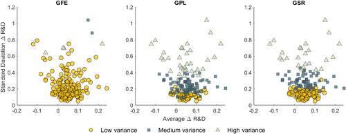
To get an intuitive understanding of the drivers of the group membership, for each firm we display the average (x-axis) and the standard deviation (y-axis) of the growth rate in R&D investments. Figure 2 displays the estimated group membership for GFE, GPL and GSR estimators for a specification with control variables. For GFE, we do not observe that differences in the average R&D growth rates are driving group membership. For GPL and GSR however, we see that the variance in the growth rates appears to correlate with group membership. This reinforces the idea that in this application, separation in the mean is weak, and the grouping is determined by the variance. We label the groups as low variance, medium variance, and high variance.

Fig. 2 R&D application: standard deviation versus average investment growth. NOTE: Estimated group membership across the average growth rate of R&D and the standard deviation of the R&D growth rates for the GFE, GPL and GSR estimators. The number of groups is set to G = 3. Group membership is determined in a model with covariates. Results are similar for the specification that does not include covariates.

Table 1 displays the estimated parameters from (28) using GFE, GSR, and GPL. To compare our results with van Ophem et al. (2019), we also estimate a fixed effects model without grouping. Columns (1)–(4) correspond to an estimation without control variables, while columns (5)–(8) display the results with control variables.

Table 1 R&D application: estimates for the output-investment relation.

	FE	GFE	GPL	GSR	FE	GFE	GPL	GSR
	(1)	(2)	(3)	(4)	(5)	(6)	(7)	(8)
One group
θ	0.169				0.098
	(0.052)				(0.064)
Low var.
θ 1		0.314	0.263	0.286		0.118	0.045	0.079
		(0.037)	(0.040)	(0.035)		(0.044)	(0.049)	(0.039)
No. firms		218	97	162		170	58	93
Med. var.
θ2		–0.050	0.237	0.160		–1.113	0.218	0.197
		(0.069)	(0.044)	(0.067)		(0.070)	(0.065)	(0.088)
No. firms		68	131	99		2	82	59
High var.
θ3		–1.199	0.036	–0.039		–0.577	–0.013	–0.010
		(0.310)	(0.133)	(0.204)		(0.287)	(0.116)	(0.139)
No. firms		5	63	30		4	36	24
Observations	8148	8148	8148	8148	4752	4752	4752	4752
N Firms	291	291	291	291	176	176	176	176
Controls	No	No	No	No	Yes	Yes	Yes	Yes

NOTE: Estimated coefficients from (28) for various models. FE indicates a fixed effect estimation that includes year fixed effects. Columns (1)–(4) show the estimated coefficients of (28) without including control variables. Columns (5)–(8) display the results when including controls. Results are based on a balanced panel dataset. Standard errors are calculated as discussed in Section 2.2 and reported in parentheses. Estimates of the group-level regression error variances are reported in the supplementary material.

Starting with the fixed effects model without groups, we confirm the findings from the literature that there is a procyclical relation between output and R&D investment. Compared to van Ophem et al. (2019), we use a balanced panel and hence the estimates differ from theirs: they find $\theta =0.263$ with a standard error of 0.034 without controls and $\theta =0.101$ with a standard error of 0.033 with controls. In the balanced panel dataset, after including the control variables, the relation between output and investment is no longer statistically significant.

Estimation of the model with different groups reveals important heterogeneity in the cyclicality patterns of R&D investment. The low-variance groups estimated by GSR provide evidence for significant procyclicality both with and without controls. The same holds for the medium-variance groups. The high-variance groups do not significantly relate the business cycle to R&D investment. GPL yields qualitatively similar results. The key finding is that after controlling for balance-sheet characteristics, the medium variance group is more procyclical compared to the low-variance groups. As expected, GFE does not find a grouping in the mean and places most firms in a single group.

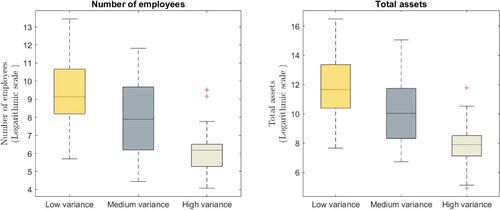
To get a better understanding of the driving factors behind the grouping, we relate the groups to a number of observed factors. We focus on the groups estimated by GSR in the model with control variables. Figure 3 shows that the low-variance group is composed of large firms (defined either by the number of employees or total assets), and the high-variance group contains small firms. The findings in Table 1 then confirm the findings by Crouzet and Mehrotra (2020) as after controlling for balance-sheet characteristics, the low-variance group, consisting of the largest firms, is found to be less procyclical relative to the medium-variance group, consisting of smaller firms.

Fig. 3 R&D application: relating groups to firm size. NOTE: The left graph displays the average number of employees as reported to shareholders. The right graph displays the firm’s total assets. The grouping of the firms corresponds to the model that includes control variables.

4.1.3 Simulation Results

We design a Monte Carlo simulation dedicated to the R&D application. The DGP is described by (28) with the true coefficients and group memberships given by the GSR estimates from the specification without control variables. We consider two DGPs. In DGP 1, we assume that the errors are normally distributed with group specific variances, and these variances are equal to the variance of the estimated regression errors in the group $\left({\widehat{\sigma }}_g^2=\frac{{\sum }_{i=1}^N{\sum }_{t=1}^T{\widehat{v}}_{\mathit{\text{it}}}^{2}1[{\widehat{g}}_i=g]}{N_{g}T-\mathit{\text{GT}}-N_g-k}\right)$. In DGP 2 each firm has a different variance that equals the estimated variance for this firm $\left({\widehat{\sigma }}_i^2=\frac{{\sum }_{t=1}^T{\widehat{v}}_{\mathit{\text{it}}}^2}{T-1}\right)$. We consider G = 3 and G = 4 for the number of groups. We calculate the average of the estimated coefficients, the root mean squared error (RMSE) and the average misclassification.

Table 2 displays the results of the Monte Carlo simulation. We first consider the case where G = 3. In DGP 1, GSR, and GPL outperform GFE in terms of misclassification. The misclassification is less than 1% for GPL and GSR, while it equals 37.5% for GFE. A higher misclassification for GFE is expected since the variance is the main feature that distinguishes the groups, and the GSR and GPL methods can exploit these differences and obtain a more accurate classification. For G = 4, the misclassification rate increases. This results from the fact that the two high variance groups are hard to separate, which is why the information criterion indicates G = 3 groups. The performance of GPL deteriorates more than that of GSR. With regard to the estimates for the coefficients θ_g , the average of the GSR and GPL estimates are close to the true values and their RMSEs are comparable. The exception is the coefficient θ₄, which again results from the fact that this group is not strongly separated from the other groups. The GFE estimates are biased because of the high degree of misclassification.

Moving to DGP 2 where the errors have individual-specific variances, we observe a substantial deterioration of the classification accuracy from GPL, while GSR is hardly affected. This confirms the theoretical results from Section 3.1. The more accurate classification results in less bias and lower RMSE values for GSR relative to GPL and GFE. Overall the results indicate that for the DGPs under consideration, GSR is able to accurately detect the grouping and estimate the coefficients of interest.

4.2 Application: Income and Democracy

We reconsider the study of Acemoglu et al. (2008) on the cross-country relation between income and democracy. After controlling for country-specific historical factors via fixed effects, Acemoglu et al. (2008) find no significant relation between income per capita and various measures of democracy. Replacing the fixed effects specification with grouped time fixed effects, Bonhomme and Manresa (2015) document a small, though statistically significant income effect. The grouping structure reflects the average democracy level over time, separating countries into a stable high-democracy group, a stable low-democracy group, and two transition groups that move toward a higher democracy level.

4.2.1 Data and Model

We use the same dataset as Acemoglu et al. (2008), Bonhomme and Manresa (2015) and follow-up work by Wang, Phillips, and Su (2018), Kim and Wang (2019), Okui and Wang (2021). The dataset contains income and democracy levels of N = 90 countries measured in five year intervals between 1970 to 2000 $(T=7$). Democracy is measured according to the Freedom House indicator, and income is measured by the log-GDP per capita obtained from the Penn World tables. Following Bonhomme and Manresa (2015), we consider the model, (29) $${\text{democracy}}_{\mathit{\text{it}}}={\theta }_1{\text{democracy}}_{\mathit{\text{it}}-1}+{\theta }_2\hspace{0.17em}\mathrm{\text{log}}\hspace{0.17em}\text{GDP}p{c}_{\mathit{\text{it}}-1}+{\alpha }_{g_{i}t}+v_{\mathit{\text{it}}}.$$(29)

4.2.2 Results: The Income Effect

Table 3 shows the estimated coefficients and the cumulative income effect for GFE, GPL, and GSR. We calculate the standard errors using a bootstrap as in Bonhomme and Manresa (2015). The estimates for GFE and GSR are similar regardless of the number of groups, and indicate a positive and significant income effect. The estimates for GPL are substantially different. When $G\ge 4$, the estimated income effect under GPL is not significant. This difference in the estimates is explained by a different grouping of the countries. The grouping of GPL emphasizes the differences in the variances, which results in a grouping that differs from the grouping of GFE and GSR. In the following section, we provide further details on the composition of the groups for the different estimators.

Table 3 Income-democracy: estimated coefficients.

G	θ1			θ2			$\frac{{\theta }_2}{1-{\theta }_1}$
	GFE	GPL	GSR	GFE	GPL	GSR	GFE	GPL	GSR
2	0.601	0.611	0.545	0.061	0.066	0.064	0.152	0.169	0.140
	(0.077)	(0.057)	(0.069)	(0.019)	(0.020)	(0.026)	(0.056)	(0.051)	(0.070)
3	0.406	0.514	0.384	0.089	0.048	0.073	0.151	0.099	0.119
	(0.118)	(0.065)	(0.099)	(0.017)	(0.023)	(0.016)	(0.040)	(0.051)	(0.044)
4	0.302	0.471	0.420	0.082	–0.003	0.069	0.118	–0.005	0.118
	(0.121)	(0.075)	(0.092)	(0.016)	(0.029)	(0.015)	(0.035)	(0.058)	(0.033)
5	0.255	0.428	0.457	0.079	–0.001	0.065	0.106	–0.002	0.119
	(0.127)	(0.088)	(0.103)	(0.015)	(0.035)	(0.017)	(0.031)	(0.062)	(0.035)
6	0.465	0.507	0.536	0.064	0.012	0.044	0.119	0.024	0.094
	(0.119)	(0.099)	(0.105)	(0.014)	(0.033)	(0.018)	(0.030)	(0.056)	(0.031)

NOTE: The table shows the estimated coefficients of equation (29) using GFE, GPL, and GSR. Bootstrap standard errors are reported in parentheses.

4.2.3 Results: Group Assignment and Interpretation

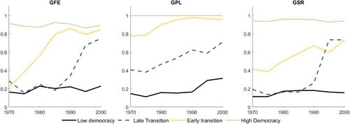
In line with Bonhomme and Manresa (2015), we focus on the specification that considers four groups of countries (G = 4). Figure 4 shows the evolution of the average democracy per group. The graph shows that the evolution of the average democracy differs substantially between groups. This suggests that the separation in the groups is mainly driven by differences in the time effects. Figure 4 indicates that the groups can be interpreted as high democracy, low democracy and two transition groups.

Fig. 4 Income-democracy: average democracy. NOTE: The graph shows the group-specific averages of democracy. Calendar years (1970–2000) are shown on the x-axis.

The composition of the groups for GFE and GSR are relatively similar. On the other hand, we observe substantial differences in the grouping for GFE and GPL. Table 4 shows the number of countries per group and the number of countries that are reallocated to a different group. If we compare GFE and GSR, we see that 19 countries (21%) are reclassified. Moreover, the reclassified countries are all assigned to the same group.

Table 4 Income-democracy: transition between groups.

		GFE
		Low	Late	Early	High
		democracy	transition	transition	democracy	Total
GSR	Low democracy	20	0	0	0	20
	Late transition	0	12	0	0	12
	Early transition	6	6	13	7	32
	High democracy	0	0	0	26	26
GPL	Low democracy	20	9	0	0	29
	Early transition	6	9	10	8	33
	Late transition	0	0	3	12	15
	High democracy	0	0	0	13	13
Total		26	18	13	33

NOTE: The table shows the total number of countries for each group for the GSR, GFE, and GPL. Additionally, it shows the number of reclassified countries.

On the other hand, for GFE and GSR, we have that 45 countries (50%) are reclassified.

4.2.4 Simulation Results

We consider the DGP described by (29). The income data are re-used from the application, and the democracy index is initialized at the initial values in the data. We consider three variants of the DGP. In each variant the coefficients and group memberships correspond to the GFE estimation results of Bonhomme and Manresa (2015) (Algorithm 2) for $G=\{3,4\}$ groups. In DGP 1, the errors v_it are drawn independently from a normal distribution with homoscedastic variance equal to the variance of the estimated regression errors. In this DGP, there is no group-level variance heterogeneity. In DGP 2, the variance of the errors is group-specific, that is $v_{\mathit{\text{it}}}\sim N(0,{\widehat{\sigma }}_{g_i}^2)$, where ${\widehat{\sigma }}_{g_i}^2$ is the estimated variance of the errors for the group that contains the country i in the empirical application. In DGP 3, variance of the errors is country-specific, so $v_{\mathit{\text{it}}}\sim N(0,{\widehat{\sigma }}_i^2)$, where ${\widehat{{\sigma }_i}}^2$ is the estimated variance for country i.

The results are shown in Table 5. For DGP 1 (homoscedastic variance) we have that the averages of the estimated coefficients are close to the true coefficients for all estimators. The classification accuracy is also largely the same. The results for DGP 2 and DGP 3 show large fluctuations of the performance of the GPL method. In DGP 3, the deterioration in the accuracy aligns with the theory developed in Section 3.1 showing that GPL is more sensitive to unit specific variances. With regard to GFE, while the theory does not make assumptions on the variance structure, it does appear that the grouped structure of DGP 2 negatively affects the classification accuracy of GFE. Overall, the GSR estimator performs well under all three DGPs.

Table 5 Income-democracy, Monte Carlo: RMSE and misclassification.

				Average			RMSE			${\widehat{g}}_i\ne g_i$ (%)
DGP	G		True	GFE	GPL	GSR	GFE	GPL	GSR	GFE	GPL	GSR
1	3	θ 1	0.406	0.395	0.400	0.396	0.054	0.060	0.055	10.15	10.98	10.21
		θ 2	0.089	0.100	0.099	0.099	0.017	0.017	0.016
	4	θ 1	0.302	0.333	0.340	0.335	0.097	0.105	0.100	11.20	12.97	11.57
		θ 2	0.082	0.089	0.089	0.089	0.015	0.015	0.015
2	3	θ 1	0.406	0.380	0.395	0.380	0.056	0.048	0.052	11.41	9.36	9.45
		θ2	0.089	0.099	0.095	0.098	0.016	0.014	0.016
	4	θ1	0.302	0.300	0.310	0.291	0.065	0.057	0.057	13.91	15.39	11.80
		θ2	0.082	0.092	0.089	0.091	0.016	0.014	0.015
3	3	θ1	0.406	0.406	0.562	0.432	0.072	0.168	0.092	10.12	27.52	12.90
		θ2	0.089	0.087	0.078	0.086	0.015	0.017	0.016
	4	θ1	0.302	0.332	0.424	0.362	0.083	0.141	0.104	9.76	25.05	12.51
		θ2	0.082	0.082	0.079	0.081	0.013	0.013	0.013

NOTE: The DGP is given by (29). The coefficients and group memberships correspond to the GFE estimates from Table 3. In DGP 1, $v_{\mathit{\text{it}}}\sim N(0,{\widehat{\sigma }}^2)$ with ${\widehat{\sigma }}^2$ the variance of the estimated regression errors in the application. In DGP 2, $v_{\mathit{\text{it}}}\sim N(0,{\widehat{\sigma }}_g^2)$, where ${\widehat{\sigma }}_g^2$ equals to the variance of the estimated regression errors in group g. In DGP 3, $v_{\mathit{\text{it}}}\sim N(0,{\widehat{\sigma }}_{(i)}^2)$, where ${\widehat{\sigma }}_{(i)}^2$ is the time averaged variance of unit i. G indicates the number of groups, θ₁ and θ₂ are from the GFE column of Table 3. The final three columns show the percentage of countries that are incorrectly classified.

5 Conclusion

We identify and estimate latent group structures based on variance heterogeneity, which can be combined with grouping based on slope coefficients or time fixed effects. Our approach circumvents a singularity in the pseudolikelihood approach by adjusting the objective function. Variance based grouping improves classification accuracy when the separation in slope coefficients or grouped fixed effects is small. In an empirical illustration of the relation between R&D and investment, we find a well-defined group structure based on the variance. Accounting for these groups, we document a heterogeneous relation between output and R&D investment that ex-post can be related to firm size.

Supplementary Materials

The supplementary material contains (A) additional numerical results for the empirical applications, (B) numerical evidence for the singularity in the pseudolikehood, (C) derivations and additional numerical results under the simplified setting of Section 3.1, proofs for Theorem 1-2, (D) a BIC criterion for the number of groups. Additionally, replication code is included for the applications and corresponding simulations in Section 4.

Acknowledgments

We thank the editor, Ivan Canay, the associate editor and the referees for their comments which helped to improve the article. We also thank Artūras Juodis, Wendun Wang, Tom Wansbeek, Stephane Bonhomme and participants of the International Association for Applied Econometrics (IAAE) conference 2022, the International Panel Data Conference 2021, the 2021 SOM PhD Conference, and the 2021 TI/UvA Workshop on Panel Data for helpful comments.

Disclosure Statement

The authors report there are no competing interests to declare.

Additional information

Funding

Jhordano Aguilar Loyo acknowledges financial support by IAAE Student Travel Grant 2022. Tom Boot acknowledges financial support by the Dutch Research Council (NWO) as part of grant VI.Veni.201E.11.

References

- Acemoglu, D., Johnson, S., Robinson, J. A., and Yared, P. (2008), “Income and Democracy,” American Economic Review, 98, 808–42. DOI: 10.1257/aer.98.3.808.
- Ando, T., and Bai, J. (2017), “Clustering Huge Number of Financial Time Series: A Panel Data Approach with High-Dimensional Predictors and Factor Structures,” Journal of the American Statistical Association, 112, 1182–1198. DOI: 10.1080/01621459.2016.1195743.
- Bachmann, R., and Bayer, C. (2014), “Investment Dispersion and the Business Cycle,” American Economic Review, 104, 1392–1416. DOI: 10.1257/aer.104.4.1392.
- Barlevy, G. (2007), “On the Cyclicality of Research and Development,” American Economic Review, 97, 1131–1164. DOI: 10.1257/aer.97.4.1131.
- Belloni, A., Chernozhukov, V., and Wang, L. (2011), “Square-Root Lasso: Pivotal Recovery of Sparse Signals via Conic Programming,” Biometrika, 98, 791–806. DOI: 10.1093/biomet/asr043.
- Bonhomme, S., Lamadon, T., and Manresa, E. (2022), “Discretizing Unobserved Heterogeneity,” Econometrica, 90, 625–643. DOI: 10.3982/ECTA15238.
- Bonhomme, S., and Manresa, E. (2015), “Grouped Patterns of Heterogeneity in Panel Data,” Econometrica, 83, 1147–1184. DOI: 10.3982/ECTA11319.
- Browning, M., and Carro, J. M. (2010), “Heterogeneity in Dynamic Discrete Choice Models,” The Econometrics Journal, 13, 1–39. DOI: 10.1111/j.1368-423X.2009.00301.x.
- Carrasco, M., Hu, L., and Ploberger, W. (2014), “Optimal Test for Markov Switching Parameters,” Econometrica, 82, 765–784.
- Crouzet, N., and Mehrotra, N. R. (2020), “Small and Large Firms over the Business Cycle,” American Economic Review, 110, 3549–3601. DOI: 10.1257/aer.20181499.
- Fabrizio, K. R., and Tsolmon, U. (2014), “An Empirical Examination of the Procyclicality of R&D Investment and Innovation,” Review of Economics and Statistics, 96, 662–675. DOI: 10.1162/REST_a_00412.
- Gu, J., and Volgushev, S. (2019), “Panel Data Quantile Regression with Grouped Fixed Effects,” Journal of Econometrics, 213, 68–91. DOI: 10.1016/j.jeconom.2019.04.006.
- Hamilton, J. D. (1991), “A Quasi-Bayesian Approach to Estimating Parameters for Mixtures of Normal Distributions,” Journal of Business & Economic Statistics, 9, 27–39. DOI: 10.1080/07350015.1991.10509824.
- Hamilton, J. D., and Lin, G. (1996), “Stock Market Volatility and the Business Cycle,” Journal of Applied Econometrics, 11, 573–593. DOI: 10.1002/(SICI)1099-1255(199609)11:5<573::AID-JAE413>3.0.CO;2-T.
- Hathaway, R. J. (1985), “A Constrained Formulation of Maximum-Likelihood Estimation for Normal Mixture Distributions,” The Annals of Statistics, 13, 795–800. DOI: 10.1214/aos/1176349557.
- Kapetanios, G. (2008), “A Bootstrap Procedure for Panel Data Sets with Many Cross-Sectional Units,” The Econometrics Journal, 11, 377–395. DOI: 10.1111/j.1368-423X.2008.00243.x.
- Kasahara, H., and Shimotsu, K. (2009), “Nonparametric Identification of Finite Mixture Models of Dynamic Discrete Choices,” Econometrica, 77, 135–175.
- Kiefer, N. M. (1978), “Discrete Parameter Variation: Efficient Estimation of a Switching Regression Model,” Econometrica, 46, 427–434. DOI: 10.2307/1913910.
- Kim, J., and Wang, L. (2019), “Hidden Group Patterns in Democracy Developments: Bayesian Inference for Grouped Heterogeneity,” Journal of Applied Econometrics, 34, 1016–1028. DOI: 10.1002/jae.2734.
- Kraiczy, N. D., Hack, A., and Kellermanns, F. W. (2015), “CEO Innovation Orientation and R&D Intensity in Small and Medium-Sized Firms: The Moderating Role of Firm Growth,” Journal of Business Economics, 85, 851–872. DOI: 10.1007/s11573-014-0755-z.
- Leng, X., Chen, H., and Wang, W. (2023), “Multi-Dimensional Latent Group Structures with Heterogeneous Distributions,” Journal of Econometrics, 233, 1–21. DOI: 10.1016/j.jeconom.2021.09.005.
- Lin, C.-C., and Ng, S. (2012), “Estimation of Panel Data Models with Parameter Heterogeneity When Group Membership is Unknown,” Journal of Econometric Methods, 1, 42–55. DOI: 10.1515/2156-6674.1000.
- Liu, R., Shang, Z., Zhang, Y., and Zhou, Q. (2020), “Identification and Estimation in Panel Models with Overspecified Number of Groups,” Journal of Econometrics, 215, 574–590. DOI: 10.1016/j.jeconom.2019.09.008.
- Lu, X., and Su, L. (2017), “Determining the Number of Groups in Latent Panel Structures with an Application to Income and Democracy,” Quantitative Economics, 8, 729–760. DOI: 10.3982/QE517.
- Lumsdaine, R. L., Okui, R., and Wang, W. (2023), “Estimation of Panel Group Structure Models with Structural Breaks in Group Memberships and Coefficients,” Journal of Econometrics, 233, 45–65. DOI: 10.1016/j.jeconom.2022.01.001.
- Miao, K., Su, L., and Wang, W. (2020), “Panel Threshold Regressions with Latent Group Structures,” Journal of Econometrics, 214, 451–481. DOI: 10.1016/j.jeconom.2019.07.006.
- Okui, R., and Wang, W. (2021), “Heterogeneous Structural Breaks in Panel Data Models,” Journal of Econometrics, 220, 447–473. DOI: 10.1016/j.jeconom.2020.04.009.
- Sarafidis, V., and Weber, N. (2015), “A Partially Heterogeneous Framework for Analyzing Panel Data,” Oxford Bulletin of Economics and Statistics, 77, 274–296. DOI: 10.1111/obes.12062.
- Schumpeter, J. A. (1939), Business cycles, New York: McGraw-Hill.
- Shalit, S. S., and Sankar, U. (1977), “The Measurement of Firm Size,” The Review of Economics and Statistics, 59, 290–298. DOI: 10.2307/1925047.
- Su, L., Shi, Z., and Phillips, P. C. (2016), “Identifying Latent Structures in Panel Data,” Econometrica, 84, 2215–2264. DOI: 10.3982/ECTA12560.
- Sun, T., and Zhang, C.-H. (2012), “Scaled Sparse Linear Regression,” Biometrika, 99, 879–898. DOI: 10.1093/biomet/ass043.
- Sun, Y. (2005), “Estimation and Inference in Panel Structure Models,” Available at SSRN 794884.
- van Ophem, H., van Giersbergen, N., van Garderen, K. J., and Bun, M. (2019), “The Cyclicality of R&D Investment Revisited,” Journal of Applied Econometrics, 34, 315–324. DOI: 10.1002/jae.2667.
- Wang, W., Phillips, P. C., and Su, L. (2018), “Homogeneity Pursuit in Panel Data Models: Theory and Application,” Journal of Applied Econometrics, 33, 797–815. DOI: 10.1002/jae.2632.
- Zhang, Y., Wang, H. J., and Zhu, Z. (2019), “Quantile-Regression-based Clustering for Panel Data,” Journal of Econometrics, 213, 54–67. DOI: 10.1016/j.jeconom.2019.04.005.