A Smooth Shadow-Rate Dynamic Nelson-Siegel Model for Yields at the Zero Lower Bound

Abstract

We propose a smooth shadow-rate version of the dynamic Nelson-Siegel (DNS) model to analyze the term structure of interest rates during a zero lower bound (ZLB) period. By relaxing the no-arbitrage restriction, our shadow-rate model becomes highly tractable with a closed-form yield curve expression. This permits the implementation of readily available DNS extensions such as allowing for time-varying parameters and the integration of macroeconomic variables. Using U.S. Treasury data, we provide clear evidence of a smooth transition of the yields entering and leaving the ZLB state. Moreover, we show that the smooth shadow-rate DNS model dominates the baseline DNS model and (shadow-rate) affine term structure models in terms of fitting and forecasting the yield curve, while it also produces plausible policy insights at the ZLB.

Keywords:

• Yield curve
• zero lower bound
• shadow-rate model
• Nelson-Siegel model

JEL Classification:

• E43
• E47
• C53
• C58
• G12

Disclaimer

As a service to authors and researchers we are providing this version of an accepted manuscript (AM). Copyediting, typesetting, and review of the resulting proofs will be undertaken on this manuscript before final publication of the Version of Record (VoR). During production and pre-press, errors may be discovered which could affect the content, and all legal disclaimers that apply to the journal relate to these versions also.

1 Introduction

Accurately modelling and forecasting the term structure of interest rates is of key importance to both market participants and financial institutions in the context of portfolio and risk management, derivatives pricing, and monetary policy. The aftermaths of the global financial crisis and the covid pandemic have highlighted that this task becomes more challenging in times of prolonged low interest rates close to the so-called zero lower bound (ZLB). This ZLB is an absorbing state and forces short-term yields to become flat and less volatile, leading to asymmetric behaviour in the entire yield curve. Unfortunately, traditional term structure models are not able to capture these changed ZLB dynamics (Christensen and Rudebusch, 2015, 2016; Bauer and Rudebusch, 2016). Hence, there is a need for tractable models that can handle the nonlinearity of the term structure of interest rates at the ZLB.

To address this issue, we propose a smooth shadow-rate version of the Nelson-Siegel model (Nelson and Siegel, 1987) that imposes the ZLB onto the yields via the shadow short-rate concept of Black (1995). Following Diebold and Li (2006), this model is turned into a forecasting device by allowing for time-varying factors and by explicitly modelling their dynamics. Just like the standard dynamic Nelson-Siegel (DNS) model, our shadow-rate version is highly tractable and, in contrast to no-arbitrage shadow-rate term structure models, neither needs computationally intensive numerical methods nor forward-rate data to be estimated. In fact, our smooth shadow-rate DNS models can simply be estimated with the two-step approach of Diebold and Li (2006) based on (nonlinear) least squares, or alternatively, with maximum likelihood and extended Kalman filtering methods by putting it in a nonlinear state-space form.

Our modelling approach explicitly allows for a smooth transition into and out of the ZLB state by means of a soft lower-bound restriction such that medium- and long-term yields, that are themselves not directly near the ZLB, still recognize the presence of a lower bound and the fact that short-term yields could be bounded. Moreover, the smooth shadow-rate DNS model easily permits the implementation of readily available DNS extensions. We illustrate and benefit from this flexibility by allowing the yield curve factors to evolve around a slowly time-varying mean (or ‘shifting endpoint’) as in van Dijk et al. (2014) and Bauer and Rudebusch (2020) to capture the seemingly non-stationary behaviour of yields.

We consider monthly U.S. zero-coupon government bond yields from August 1971 to December 2023, which experienced a prolonged period of being subject to the ZLB from December 2008 to December 2015 and from April 2020 to March 2022. Our empirical analysis shows that the smooth shadow-rate DNS model provides a better in-sample fit than the DNS model in terms of root mean squared fitting errors (RMSE). The overall improvement in RMSE is about 12.5% over the total period and 57.5% over the ZLB period. Furthermore, we find clear evidence of a smooth lower-bound restriction, indicated by better fitting performance for smoother approximation functions relative to non-smooth or less smooth ones. This implies that the yield curve as a whole gradually enters and leaves the ZLB state, which corroborates with the findings of Swanson and Williams (2014) that medium-term yields only started to be constrained by the ZLB from late 2011 onward. Likewise, it implies that the yield curve slowly recovers from the ZLB state, which is consistent with gradual monetary policy normalization (Hördahl and Tristani, 2019).

Next, we show that the original DNS model lacks the ability to account for the compression of yield volatility at the ZLB, leading to improbably high positive probabilities of negative projected short- and medium-term yields. Meanwhile, the smooth shadow-rate DNS model imposes the condition that yields must be non-negative and therefore accurately replicates the low yield volatility. Consequently, the smooth shadow-rate DNS model produces more accurate forecasts than the baseline DNS model and also than the (shadow-rate) affine term structure model. This improvement is generally strongest for short-term yields during the ZLB period. Again, the outperformance is more pronounced for models with a smoother approximating function, indicating that the forecast gains really stem from the smooth lower-bound restriction. The imposition of shifting endpoints leads to additional prediction gains, showing that incorporating long-run trends in yield dynamics is complementary to accounting for the ZLB via our smooth lower-bound approach.

Finally, our model delivers valuable output that can be useful for shaping policy expectations. In particular, it produces shadow short-rate estimates to gauge the stance of unconventional monetary policy, it can provide liftoff-horizon estimates to indicate when the policy rate starts to diverge again from the ZLB, and it facilitates a way to construct expected short-rate and term premia estimates at the ZLB that resemble existing alternatives. Given that the yield forecasts and policy output can simply be obtained with (nonlinear) least squares, our modelling approach is highly applicable and attractive to practitioners and policy makers.

Our work is closely related to and builds on two strands of term structure modelling literature. First, it relates to the existing literature on shadow-rate term structure models that respect the ZLB. Specifically, shadow-rate models impose the condition that the observed short rate is the maximum of a lower bound, often assumed zero, and a shadow short rate that would prevail in a world without physical currency and hence can become negative. Most, if not all, literature on shadow-rate models apply this concept in the framework of the theoretically consistent class of (no-arbitrage) affine term structure models (ATSM) (Vasicek, 1977; Duffie and Kan, 1996; Dai and Singleton, 2000). However, this implementation does not lead to closed-form analytic bond price formulas such that numerical methods (Gorovoi and Linetsky, 2004; Kim and Singleton, 2012) or ZLB bond price approximations (Krippner, 2013; Christensen and Rudebusch, 2015, 2016; Wu and Xia, 2016; Bauer and Rudebusch, 2016) are required. Despite these advances, shadow-rate ATSM estimation remains computationally intensive, especially with a large number of parameters as in macro-finance models (Bauer and Rudebusch, 2016). Hence, we contribute to this strand of literature by providing a reduced-form shadow-rate model that is highly tractable, even in a large dimensional parameter space. This tractability comes at the cost of not necessarily satisfying the no-arbitrage restriction, but literature generally finds mixed results on the empirical importance of no-arbitrage restrictions and empirical difference of the DNS and arbitrage-free models (see, for example, Duffee, 2011; Coroneo et al., 2011; Krippner, 2015). Joslin et al. (2011) argue that the specification of the physical process of the factors instead are the key to accurate yield forecasts.

Second, our work is related to the strand of literature that employs reduced-form models for the term structure of interest rates. Notably, the DNS model of Diebold and Li (2006) gained popularity due to its simplicity, stable estimation and good in-sample and out-of-sample performance. Moreover, the DNS model can be easily augmented in various directions like the integration of macroeconomic variables (Diebold et al., 2006; Koopman and van der Wel, 2013; Coroneo et al., 2016), adding time-varying volatility or factor loadings (Koopman et al., 2010), shifting endpoints (van Dijk et al., 2014), or time-varying parameter vector autoregressions (Hevia et al., 2015; Byrne et al., 2017). However, applying the reduced-form DNS model in the context of shadow-rate term structure modelling has, to the best of our knowledge, not been considered. Our work therefore bridges the gap between the shadow-rate class and reduced-form class of term structure models to obtain a model that obeys the ZLB and at the same time remains highly tractable. Due to this tractability, our novel shadow-rate DNS model has as appealing feature that there is the flexibility to easily incorporate the aforementioned model extensions.

The remainder of this paper is as follows. Section 2 introduces our smooth shadow-rate version of the DNS model. Section 3 discusses the data and displays our empirical analysis in terms of in-sample and out-of-sample performance as well as some policy insights at the ZLB. Section 4 concludes.

2 Smooth shadow-rate dynamic Nelson-Siegel model

In this section, we first discuss the dynamic Nelson-Siegel approach to yield curve modelling and forecasting in Section 2.1, which is augmented to account for the zero lower bound via a smooth shadow-rate adaption in Section 2.2. Then, in Section 2.3, we exploit the tractability of our model by incorporating different shifting-endpoint extensions.

2.1 Dynamic Nelson-Siegel model

The term structure of interest rates can take on a variety of different shapes such as upward sloping, downward sloping, humped and inverted humped. A parsimonious yield curve expression that is able to capture all these different shapes is the functional form proposed by Nelson and Siegel (1987), which has been popularized by Diebold and Li (2006) as a forecasting device. Specifically, they extend the model to allow for time-varying factors, resulting in the expression(1) $$y_t(\tau )={\beta }_{1t}+{\beta }_{2t}\left(\frac{1-e^{-\lambda \tau }}{\lambda \tau }\right)+{\beta }_{3t}\left(\frac{1-e^{-\lambda \tau }}{\lambda \tau }-e^{-\lambda \tau }\right),$$(1) where $y_t(\tau )$ is the yield of a zero-coupon bond at time t with time to maturity τ, λ is the factor loading parameter, and ${\beta }_{1t},{\beta }_{2t}$ and ${\beta }_{3t}$ are latent time-varying factors, which have the interpretation of level, slope and curvature, respectively. These factor interpretations are explicitly imposed by their factor loading structure (see, for example, Diebold and Li, 2006). Following Diebold and Li (2006), we set λ equal to 0.0609 such that it maximizes the curvature loading at a maturity close to 30 months. Alternatively, λ could be estimated as one of the parameters by casting the model into a linear state-space form as in Diebold et al. (2006) (see Online Appendix A for further details). The model-implied short rate r_t is given by the sum of the level and slope factor, that is, $r_t=\underset{\tau \to 0}{\lim }{y}_t(\tau )={\beta }_{1t}+{\beta }_{2t}$.

To model the dynamics of the latent factors, we follow Diebold and Li (2006) and van Dijk et al. (2014) and adopt univariate first-order autoregressions given by(2) $${\beta }_{k,t}={\mu }_k+{\psi }_k({\beta }_{k,t-1}-{\mu }_k)+{\eta }_{k,t},$$(2) for k = 1, 2, 3, with the autoregressive coefficients satisfying $\left|{\psi }_k\right|<1$ to ensure stationarity. The unconditional mean is denoted by μ_k and the error terms ${\eta }_{k,t}$ have zero mean and variance ${\sigma }_k^2$ and are mutually and serially independent at all leads and lags. Given these factor dynamics, it becomes straightforward to generate h-step ahead forecasts of ${\beta }_{k,t+h}$ by forward iteration of equation (2), after which we obtain h-step ahead yield curve forecasts by plugging the factor forecasts into equation (1). This procedure to yield curve modelling and forecasting is known as the dynamic Nelson-Siegel (DNS) approach and has proven to be successful in various studies (see, among others, Diebold and Li, 2006; De Pooter, 2007; van Dijk et al., 2014).

Given a set of N observed yields at time t, collected in the observation vector ${\mathit{y}}_t^o=(y_t^o({\tau }_1),\dots ,y_t^o({\tau }_N))\prime$, and by exploiting the linear factor structure in equation (1) for a pre-fixed value of λ, the latent factors can be estimated with a cross-sectional regression at each time t (Diebold and Li, 2006), that is,$${\widehat{\beta }}_t={(\mathit{\Lambda }(\lambda )\prime \mathit{\Lambda }(\lambda ))}^{-1}\mathit{\Lambda }(\lambda )\prime {\mathit{y}}_t^o,$$for $t=1,\dots ,T$, where ${\widehat{\beta }}_t=({\widehat{\beta }}_{1t},{\widehat{\beta }}_{2t},{\widehat{\beta }}_{3t})\prime$ is the 3 × 1 vector with latent factor estimates and $\mathbf{\Lambda }(\lambda )$ is the $N\times 3$ factor loading matrix given by$$\mathit{\Lambda }(\lambda )=\left(\begin{array}{ccc}1& \frac{1-{\mathrm{e}}^{-\lambda {\tau }_1}}{\lambda {\tau }_1}& \frac{1-{\mathrm{e}}^{-\lambda {\tau }_1}}{\lambda {\tau }_1}-e^{-\lambda {\tau }_1}\\ ⋮& ⋮& ⋮\\ 1& \frac{1-{\mathrm{e}}^{-\lambda {\tau }_N}}{\lambda {\tau }_N}& \frac{1-{\mathrm{e}}^{-\lambda {\tau }_N}}{\lambda {\tau }_N}-e^{-\lambda {\tau }_N}\end{array}\right).$$

These factor estimates can in turn be used to estimate the univariate autoregressions in (2) with ordinary least squares (OLS). Interest rates (and its derived factors) are, however, highly persistent, inducing a small-sample bias in the OLS estimator of the coefficients (Bauer et al., 2012). As a result, the factors are estimated to be less persistent than they truly are. Therefore, we use the analytic bias approximation of Pope (1990) to correct the biased OLS estimates for μ_k and ψ_k , while we ensure stationarity via the stationary-adjustment approach of Kilian (1998).

2.2 Imposing a smooth lower-bound restriction

On its own, the DNS model does not impose the condition that yields are non-negative and, consequently, assumes that the yield curve behaves the same in low interest-rate as in high interest-rate environments. However, Black (1995) notes that the observed short rate in the market cannot become (too) negative due to the presence of a physical currency with a natural interest rate of zero (or, in practice, close to zero due to transaction and storage costs). Therefore, the short rate r_t is the maximum of a lower bound r_LB and a shadow short rate s_t that would prevail in a world without the option of physical currency, that is, $r_t=\max (r_{LB},s_t)$. The value of r_LB could either be pre-specified (for instance, at 0%) or estimated as a free parameter. In fact, a time-varying lower bound could also be accommodated, which is more plausible for some countries, for example in Europe (see, among others, Kortela, 2016; Lemke and Vladu, 2017; Wu and Xia, 2020).

By assuming that all yields are restricted by the same lower bound, we generalize this idea for the yield curve such that(3) $${\underset{¯}{y}}_t^Z(\tau )=r_{LB}+\max (0,y_t(\tau )-r_{LB}),$$(3) where ${\underset{¯}{y}}_t^Z(\tau )$ is called the zero lower bound (ZLB) yield and $y_t(\tau )$ is called the shadow yield. This assumption is also implicitly made in shadow-rate affine structure models (see, for instance, Christensen and Rudebusch, 2015). Clearly, this is a more stringent restriction for short-term yields as the yield curve is generally upward sloping, even though longer-term yields could still be affected by unconventional monetary policy (Wright, 2012; Swanson and Williams, 2014). Plugging equation (1) as shadow yield into equation (3), results in a DNS model that imposes yields to be equal or larger than the lower bound r_LB and for which the shadow short rate is equal to $s_t={\beta }_{1t}+{\beta }_{2t}$. We refer to this model as the shadow-rate DNS (B-DNS) model, in the spirit of Black (1995).

This direct lower bound approach assumes that yields are either behaving in a traditional way above r_LB or are flat and equal to r_LB . That is, the B-DNS model is non-smooth with a kink at r_LB that separates yields into two possible states, just as in a regime-switching term structure model with a ZLB state (Christensen, 2015). Consequently, an interest rate close to but above the lower-bound value (say, 0.25%) behaves similarly as when it is further away from the lower bound (say, 4%). It seems more plausible, though, that the asymmetry of the ZLB already starts to present at small but positive interest-rate levels close to the lower bound (for example, at 1%). This is particularly relevant for medium-term yields that are themselves not directly near the ZLB, but still experience the asymmetry caused by the restricted short-term yields. Indeed, Swanson and Williams (2014) show that one- and two-year yields also became affected by the ZLB in the U.S from late 2011 onwards, while Grisse (2023) shows that uncertainty of the lower-bound value also influences longer-term yields. Therefore, we introduce a smoother transition between a high interest-rate state and the ZLB state. This also conforms to the empirically observed gradual monetary policy normalization and slow recovery from the ZLB (Hördahl and Tristani, 2019).

To allow for a more gradual transition, we consider a smooth approximation function of the max function in equation (3), which we denote by $f(·)$, resulting in the smooth ZLB yield curve expression(4) $${\underset{¯}{y}}_t(\tau )=r_{LB}+f(y_t(\tau )-r_{LB}).$$(4)

There exist various functions $f(·)$ that could be used for this approximation of which we consider three. First, we follow Feunou et al. (2022) and consider the function $f_G(x)=x\Phi (x)+\varphi (x)$ that could be obtained as the antiderivative of $\Phi (·)$, where $\Phi (·)$ and $\varphi (·)$ are the cumulative and probability density functions of the standard normal distribution, respectively. This specific function resembles the ZLB forward-rate approximation of Krippner (2013) and Wu and Xia (2016) in the context of no-arbitrage shadow-rate models (see Online Appendix B for further details). Second, we consider the softplus function $f_S(x)=\hspace{0.17em}\ln \hspace{0.17em}(1+e^x)$, which is smoother than $f_G(x)$ and has been widely used as a smooth activation function in the context of artificial neural networks (see, among others, Glorot et al., 2011). Third, we consider $f_E(x)=x/(1-e^{-x})$, which is even smoother than $f_G(x)$ and $f_S(x)$. The advantage of the reduced-form DNS framework is that we can directly impose these functions onto the yield curve without the need for numerical integration. Meanwhile, the ZLB forward-rate approximation in no-arbitrage shadow-rate models requires the computation of an integral to obtain the corresponding ZLB yield curve.

The left panel in Figure 1 shows the different smooth approximations $f_G(x),f_S(x)f_E(x)$ of the max function, indicating that $f_G(x)$ is the least smooth and closest to the max function, followed by $f_S(x)$ and then $f_E(x)$. That being said, it is also possible to alter the smoothness of each function by a scaling factor γ via $\gamma f(x/\gamma )$. The right panel in Figure 1 shows the function $\gamma f_G(x/\gamma )$ for a range of values of γ, highlighting that a higher (smaller) value of γ results in a less (more) noticeable kink. Clearly, the different approximation functions could be brought closer to each other for specific values of γ, although they are never exactly the same as differences remain around zero, with decaying differences toward both ends. Given the diversity of the baseline smooth approximation functions, we focus on the three cases without additional scaling in our main analysis.

Taking each of the approximating functions and plugging them into equation (4) provides the smooth ZLB yield curve expressions(5) $${\underset{¯}{y}}_t^G(\tau )=r_{LB}+(y_t(\tau )-r_{LB})\Phi \left(y_t(\tau )-r_{LB}\right)+\varphi \left(y_t(\tau )-r_{LB}\right),$$(5) (6) $${\underset{¯}{y}}_t^S(\tau )=r_{LB}+\hspace{0.17em}\ln \hspace{0.17em}\left(1+e^{y_t(\tau )-r_{LB}}\right),$$(6) (7) $${\underset{¯}{y}}_t^E(\tau )=r_{LB}+\frac{y_t(\tau )-r_{LB}}{1-e^{-(y_t(\tau )-r_{LB})}},$$(7) which we refer to as the smooth shadow-rate DNS model with Gaussian-based approximation function (SB_G -DNS), the softplus approximation function (SB_S -DNS), and the inverse exponentially-based approximation function (SB_E -DNS), respectively.

Given the observation vector ${\mathit{y}}_t^o$ and pre-fixed values for the lower bound r_LB and factor loading λ, the latent factors can be estimated using nonlinear least squares (NLS) at each time t, that is,$${\widehat{\beta }}_t=\text{arg}\hspace{0.17em}{\min }_{{\beta }_t}\sum _{i=1}^N(y_t^o({\tau }_i)-{\underset{¯}{y}}_t^X({\tau }_i){)}^2,$$for $t=1,\dots ,T$, and $X\in \{Z,G,S,E\}$, with the model-implied ZLB yields for Z given by B-DNS in equation (3) and for G, S and E by SB-DNS in (5), (6) and (7), respectively. Similarly as for the DNS model, the dynamics of the estimated factors are modelled as univariate AR(1) processes and estimated using OLS with a bias-correction and stationary adjustment. This two-step estimation approach highlights how easily our (smooth) shadow-rate DNS models can be implemented and estimated, making it highly applicable and attractive to practitioners. The (smooth) shadow-rate DNS models could alternatively be cast into a nonlinear state-space form and be estimated with maximum likelihood estimation in combination with the extended Kalman filter. For further details of this approach, see Online Appendix A.

2.3 Shifting-endpoint extensions

To demonstrate the ease of extending the smooth shadow-rate DNS model, we consider several other dynamic specifications for the factors. In these specifications, we allow the yield curve factors to evolve around a slowly time-varying mean (or ‘shifting endpoint’) as in van Dijk et al. (2014) and Bauer and Rudebusch (2020). By doing so, we can assess whether shifting endpoints are able to replicate the yield curve asymmetry at the ZLB and also how well these non-stationary dynamics are able to complement our smooth shadow-rate model. To accommodate this feature, we follow van Dijk et al. (2014) and consider two different specifications for the time-varying mean of the latent factors.

First, we adopt the approach that the mean ${\mu }_{k,t}$ is generated by the exponential smoothing recursion(8) $${\mu }_{k,t}=\alpha {\beta }_{k,t-1}+(1-\alpha ){\mu }_{k,t-1},$$(8) for k = 1, 2, 3, where ${\mu }_{k,1}={\beta }_{k,1}$ and $0<\alpha <1$ is the decay parameter, which is set to $\alpha =0.1$ as in van Dijk et al. (2014). By substituting equation (8) into equation (2) and using the estimates of β_t , we can estimate the dynamics of the factors and construct the corresponding h-step ahead forecasts of ${\beta }_{k,t+h}$. Following van Dijk et al. (2014), we consider two variants of this approach: (i) exponential smoothing for the level factor only and AR(1) dynamics for the slope and curvature factors (labeled as ESL), and (ii) exponential smoothing for all three factors (labeled as ESLSC).

Second, the shifting endpoints could be linked to exogenous measures of macroeconomic trends such as in van Dijk et al. (2014) and Bauer and Rudebusch (2020). Indeed, there is ample evidence that long-run macroeconomic trends play a key role in determining interest rate levels (see, among others, Del Negro et al., 2017, 2019; Christensen and Rudebusch, 2019). We follow van Dijk et al. (2014) and use exponentially-smoothed realized inflation and industrial production (IP) growth, indicated as ${\pi }_t^{ES}$ and ${\zeta }_t^{ES}$, respectively. To properly account for data revisions and publication delays in the forecasting exercise, we use real-time vintage data of the monthly consumer price index and IP index from the Federal Reserve Bank of Philadelphia, which are then transformed into monthly growth rates. Given the noisiness of these growth rates, we use $\alpha =0.01$ for the exponential smoothing. Then, we run the regressions$$\begin{array}{c}{\beta }_{1,t}={\theta }_{1,0}+{\theta }_{1,1}{\pi }_t^{ES}+{\xi }_{1,t},\\ {\beta }_{2,t}={\theta }_{2,0}+{\theta }_{2,1}{\zeta }_t^{ES}+{\xi }_{1,t},\end{array}$$using the estimates of β_t , after which we construct the shifting endpoints as ${\mu }_{1,t}={\theta }_{1,0}+{\theta }_{1,1}{\pi }_t^{ES}$ and ${\mu }_{2,t}={\theta }_{2,0}+{\theta }_{2,1}{\zeta }_t^{ES}$, extrapolating that ${\pi }_t^{ES}$ and ${\zeta }_t^{ES}$ remain constant at their end-of-sample values. Again, after plugging in the specifications for ${\mu }_{1,t}$ and ${\mu }_{2,t}$ into equation (2), we can construct h-step ahead forecasts of ${\beta }_{k,t+h}$. Following van Dijk et al. (2014), we consider two variants of this approach: (i) smoothed realized inflation for the level factor only and AR(1) dynamics for the slope and curvature factors (labeled as RZI), and (ii) RZI plus smoothed realized IP growth for the slope factor and AR(1) dynamics for the curvature factor (labeled RZIG).

3 Empirical results

In this section, we present the empirical results related to our smooth shadow-rate DNS models. We first provide details of the chosen dataset in Section 3.1. The in-sample results are discussed in Section 3.2, followed by an examination of the shortcomings of the traditional DNS model during ZLB periods in Section 3.3. The baseline forecasting results are presented in Section 3.4 and the shifting-endpoint forecasting results in Section 3.5. Lastly, in Section 3.6, we examine how our model is able to provide policy insights during ZLB periods.

3.1 Data description

In our empirical application, we consider U.S. Treasury zero-coupon bond yields for seventeen maturities. Specifically, we consider the same set of maturities that are used by Diebold and Li (2006) and van Dijk et al. (2014), namely 3, 6, 9, 12, 15, 18, 21, 24, 30, 36, 48, 60, 72, 84, 96, 108 and 120 months. The yields are obtained from the monthly yield data set of Liu and Wu (2021), which is constructed based on a non-parametric kernel smoothing method. Our sample period runs from August 1971 (when the first ten-year bonds were issued) to December 2023, resulting in 629 time series observations.

Figure 2 shows the time series of yields for four selected maturities over the total sample period (left figure) and the period after the Global Financial Crisis (GFC) of 2007-2008 (right figure). The gray shaded areas in the figure correspond to the periods where the U.S. federal funds rate is below 25 basis points, meaning that yields are close to the ZLB. The figure shows that long-term yields are generally above short-term yields, corroborating the stylized fact that the yield curve is, on average, upward sloping. Moreover, short-term yields have been close to the ZLB for a prolonged period of time after the GFC. Subsequent to this ZLB period, yields started to increase again until the covid pandemic hit, which brought yields back to the ZLB in April 2020, until the final liftoff in April 2022. During these ZLB periods, short-term yield volatility is much smaller than long-term yield volatility, highlighting the volatility compression that is observed at the ZLB. Overall, these changes in dynamics indicate the need of a term structure model that accounts for the yield asymmetry and volatility compression at the ZLB.

3.2 In-sample model fit

We assess the in-sample fit across models in terms of their root mean squared fitting errors (RMSEs), which are given in Table 1 for the total sample period (Panel A), the pre-ZLB period (Panel B), the ZLB period (Panel C) and the post-ZLB period (Panel D). The table presents the RMSEs for the DNS model and its (smooth) shadow-rate adaptions: B-DNS, SB_G -DNS, SB_S -DNS and SB_E -DNS. For comparison, we also include the less tractable closest affine term structure model and its shadow-rate counterpart: the arbitrage-free Nelson-Siegel (AFNS) model of Christensen et al. (2011) and the shadow-rate AFNS model of Christensen and Rudebusch (2015), see Online Appendix B for further details on their model specification and estimation. Following the recommendation of Christensen and Rudebusch (2016) for U.S. government bond yields, we estimate all shadow-rate models with a fixed lower-bound specification of 0%. The in-sample fit for different lower-bound specifications of r_LB and scaler values γ in the smooth approximation functions are explored in Online Appendices C and D, respectively.

There are three key findings based on our comparison. First, the smooth shadow-rate DNS models produce considerably lower RMSE values than the DNS model for all sample periods. In particular, the overall improvement in RMSE of the SB_E -DNS model relative to the DNS model is about 12.5% for the total period, 1.4% for the pre-ZLB period, 57.5% for the ZLB period and 5.7% for the post-ZLB period. Unsurprisingly, the accuracy gains are thus most pronounced during low interest-rate periods (Panel C and D), while the fit is about the same (or only marginally better) during high interest-rate periods (Panel B). These improvements in fit are observed for both short- and long-term yields at the ZLB, ranging from an improvement of 50.4% for the three-month yield to 63.3% for the ten-year yield. Hence, the imposition of the smooth shadow-rate framework leads to a substantial gain in yield curve fit across all maturities.

Second, when comparing across (smooth) shadow-rate specifications, it stands out that the smoothest approximating function in equation (7) (that is, SB_E -DNS) produces the best fit. In particular, the SB_E -DNS model has an overall in-sample fit that is about 30.4% more accurate than for the SB_G -DNS model and 11.4% for the SB_S -DNS model. This generally holds for all periods and maturities, except for the three-month yield during the post-ZLB period. Hence, we find clear evidence of a more gradual transition into the ZLB state. Meanwhile, the B-DNS model has a highly similar in-sample fit as the DNS model, indicating that the improvements in fit truly come from the imposition of the smooth lower-bound restriction and not from a hard lower bound.

Third, the smooth shadow-rate models also generate a better overall in-sample fit than the (B-)AFNS models, ranging from a 32.8% improvement in total RMSE during the ZLB period to a 55% during the post-ZLB period. These gains mostly stem from the poor in-sample fit of the (B-)AFNS models for short-term yields, which has also been documented by Christensen and Rudebusch (2016). Still, (B-)AFNS performs somewhat better for medium-term yields during the pre-ZLB and post-ZLB periods. Consistent with Christensen and Rudebusch (2016), we find that B-AFNS performs slightly better than AFNS during the ZLB period, but rather similarly during the other periods. Overall, our smooth shadow-rate DNS models are highly competitive in terms of in-sample fit with the less tractable class of (shadow-rate) affine term structure models that satisfy no-arbitrage.

To illustrate how much the baseline and smooth shadow-rate DNS models deviate in terms of dynamics, Figure 3 compares the estimated yield curve factors from the DNS and SB_X -DNS models for $X\in \{G,S,E\}$. The estimated level factors are rather similar across the DNS and different SB-DNS models, with only marginal differences during the ZLB periods that are somewhat larger for a smoother approximation and thus largest for SB_E -DNS. Noticeably, the level factors exhibit a downward trend since the 1990s, which clearly motivates the choice to also consider shifting endpoints.

For the estimated slope and curvature factors, we find more pronounced differences between the DNS and different SB-DNS models. In particular, the SB-DNS models generate a steeper yield curve slope at the ZLB than the DNS model, with the steepest slope occurring for SB_E -DNS. This follows from the fact that the smooth shadow-rate models allow for a shadow yield curve that is not restricted by a lower bound and therefore can become negative, while the corresponding model-implied yields still obey the ZLB. Consequently, the shadow slope factor is able to move more freely, whereas the DNS slope factor cannot become too negative as that would deteriorate the fit of the bounded short-term yields. In a similar fashion, the estimated curvature factor of the DNS model is restricted to move at the ZLB, while the ones of the SB-DNS models behave more freely. The differences between the estimated shadow short rate and short rate proxies the ZLB wedge measure, which gauges how tightly the ZLB restricts the yield curve (see Bauer and Rudebusch (2016) for further details). As expected, these wedges are larger during ZLB periods, but they are also sizable when yields are close to zero during 2002 through 2005.

3.3 Capturing yield curve behaviour at the zero lower bound

This section examines the (in)ability of the DNS model to generate plausible future yield curve behaviour at the ZLB and compares this to that of the different SB-DNS models. We first examine conditional probabilities of negative projected yields three months ahead. Figure 4 shows such conditional probabilities for the DNS model based on $10,000$ simulations at each observation date t. Prior to the GFC, most yields have negligible probabilities of turning into negative territory, except for the three-month yield during 2002-2005. However, the probabilities of the three-month and two-year yields increase substantially during the ZLB period. In fact, during the covid pandemic, even the ten-year yield shows positive probabilities above 0.2. Hence, by ignoring the ZLB, the DNS model is not able to generate realistic future interest rate paths, as U.S. interest rates did not become negative during our sample with a minimum of 0.12 for the two-year yield and 0.53 for the ten-year yield. These unlikely high positive probabilities of negative interest rates are also found for the affine term structure model class, see Christensen and Rudebusch (2015, 2016) and Bauer and Rudebusch (2016), among others. Meanwhile, for the different (S)B-DNS models, the conditional probability of yields becoming negative is, by construction, equal to zero.

Next, we assess whether the DNS model is able to capture the yield volatility compression at the ZLB. Figure 5 shows the conditional volatility of projected yields three-months ahead obtained from the DNS, B-DNS and different SB-DNS models, based on 10,000 simulations at each observation date t. For comparison, we also include a realized-volatility (RV) measure, where we follow Christensen and Rudebusch (2016) and compute rolling standard deviations of daily yield changes over the number of trading days in the next 91-day window. Due to the linearity of the DNS model and the stationary dynamics of the factors, the DNS model produces constant yield volatility, as can be seen in Figure 5. However, for both the three-month and two-year yields, the RV measure decreases drastically after the GFC to a level of 0.1 to 0.2. The different SB-DNS models are able to replicate this decrease in volatility and stick more closely to the RV measure, especially the smoother SB_S -DNS and SB_E -DNS models, albeit with some divergence of the series between the two ZLB periods. The B-DNS model is only partly able to capture the volatility compression, whereas it converges rather quickly to the constant volatility level of the DNS model. These shortcomings in capturing low yield volatility are also found for the affine model class (Christensen and Rudebusch, 2015, 2016).

3.4 Forecasting results

In this section, we examine the out-of-sample performance of the (smooth) shadow-rate DNS models. We conduct an expanding-window forecasting exercise with an initial estimation sample from August 1971 to July 1991 (240 observations). By adding one month of observations each time, we conduct a total of 390 estimations per model. For each estimation sample, we assume a fixed lower-bound specification of 0%, with relaxations of this in Online Appendix C. Then, at each end date of the estimation sample, we construct six-months-ahead (h = 6), one-year-ahead (h = 12) and two-years-ahead (h = 24) forecasts. This results in a total of 384, 378 and 366 forecasts for h = 6, h = 12 and h = 24, respectively. To evaluate the forecasts, we compute the root mean squared forecast errors (RMSFEs). We refer to Online Appendix D for an empirical comparison of the different values of γ across approximation functions in the context of forecasting the yield curve.

Table 2 displays the relative RMSFEs of the (S)B-DNS and (B-)AFNS models compared to the DNS model across forecast horizons and maturities for the total out-of-sample period (Panel A), the pre-ZLB period (Panel B), the ZLB period (Panel C) and the post-ZLB period (Panel D). Besides the model-based forecasts, we also include the random walk, which is known to be a hard-to-beat benchmark for yields (Duffee, 2002). A value smaller (larger) than one indicates outperformance (underperformance) of the given model over the DNS model.

Most prominently, we find that the SB-DNS models significantly outperform the DNS model for short- and medium-term yields at all forecast horizons, with the strongest improvements for short-horizon forecasts (h = 6). As expected, the forecasting gains are most pronounced when the ZLB is binding, namely during the ZLB period in Panel C. Moreover, these improvements are most striking for the shadow-rate DNS model with the smoothest approximation function (that is, SB_E -DNS), which reaches an improvement in RMSFEs as large as 36% for the three-month yield forecasts during the ZLB period. Meanwhile, the SB-DNS models perform rather similar as the DNS model during the pre- and post-ZLB period, except for h = 24 during the post-ZLB period, where the SB-DNS models do slightly better. The B-DNS model performs similarly as the DNS model for all maturities, horizons and evaluation periods, indicating that the forecast gains really stem from the smooth lower-bound restriction.

Moving to the other benchmarks, the SB-DNS models also outperform the B-AFNS and especially AFNS models for short- and medium-term yields and all forecast horizons, especially during the ZLB period. However, for longer maturities, the (B-)AFNS models often perform better than our smooth shadow-rate models, which could be due to the yield adjustment term in the (B-)AFNS model (Christensen et al., 2011) that is particularly prominent for long-term yields. Comparing AFNS with B-AFNS indicates that the former outperforms the latter during the post-ZLB period, while it is the other way around during the pre-ZLB and ZLB period. The random walk generally performs better than the model-based forecasts, except for some longer horizon forecasts (h = 24). Overall, our smooth shadow-rate models are competitive to well-known existing benchmarks like the no-arbitrage (shadow-rate) affine term structure model class. This implies that practitioners interested in constructing accurate yield forecasts at an extremely low computational cost could opt for our smooth shadow-rate DNS approach, instead of the less tractable shadow-rate affine term structure model. Moreover, our approach forms a flexible baseline setting for further extensions of possibly improving yield forecasts as discussed in the next section.

3.5 Forecasting results for shifting-endpoint specifications

To highlight the ease and relevance of extending our models, Table 3 shows the relative RMSFEs of the DNS and SB_E -DNS model with different shifting-endpoint extensions relative to the baseline DNS model with AR(1) factor dynamics. We focus solely on the SB_E -DNS variant given its good performance in the previous sections, where the shifting-endpoint results for the other SB-DNS models are given in Online Appendix E. The relative RMSFEs are shown across horizons and maturities over the same four evaluation periods as in Table 2 and are based on a similar expanding-window forecasting exercise. A value smaller (larger) than one indicates outperformance (underperformance) of the given model over the DNS model with AR(1) dynamics, where the bold numbers indicate that the SB_E -DNS model with a specific shifting-endpoint specification outperforms the DNS model with the same specification. Robustness checks towards the exponential-smoothing parameter α in the SB_E -DNS model are done in Online Appendix F.

Table 3 shows that the shifting-endpoint extensions produce only marginal forecast improvements for the DNS model. This follows from the fact that our baseline DNS model uses a bias-corrected estimator for the autoregressive coefficients, already handling the high persistence of the factors and making the forecast gains of the shifting-endpoint extensions relatively small. These results thus show bias-correction as a competitor to shifting endpoints for pure forecasting purposes, both capturing differently the high persistence in the series. Indeed, Online Appendix G shows that the bias-correction leads to substantial forecasting gains for the DNS model. During the ZLB period, however, we do observe considerable forecast improvements over the baseline DNS model for the exponential smoothing of all factors (ESLSC) and the smoothed macroeconomic realizations for level and slope factors (RZIG), highlighting that these extensions of DNS are particularly useful when the ZLB is binding.

Zooming in on the SB_E -DNS model shows that the imposition of the smooth lower-bound restriction additionally improves performance on top of the shifting-endpoint extensions (as indicated by the many bold numbers). Just as for the baseline SB_E -DNS model, these improvements are particularly large during the ZLB period and for short- and medium-term yields, although there are also large gains for ESLSC for longer maturities. The out-of-sample performance of SB_E -DNS with shifting endpoints is also more accurate than of (B-)AFNS given in Table 2. Overall, this shows that the shifting-endpoint extension and smooth lower-bound restriction are complementary, producing the largest improvements relative to the traditional DNS and (shadow-rate) affine models when they are simultaneously employed. More generally, this emphasizes the ease and flexibility of extending our smooth shadow-rate models to further improve forecast performance.

3.6 Policy insights at the zero lower bound

Lastly, we provide some policy insights at the ZLB that can be obtained from our SB-DNS models. We first examine and compare the estimated shadow short rates, which some advocate to be a useful measure of the stance of unconventional monetary policy at the ZLB (Krippner, 2013; Wu and Xia, 2016; Damjanović and Masten, 2016; Johannsen and Mertens, 2021). These estimates are highly sensitive to choices in their estimation such as the model specification and the used data (Christensen and Rudebusch, 2015, 2016; Krippner, 2020), meaning that they should always be employed with caution.

The left panel of Figure 6 shows the estimated shadow short rates from the SB-DNS models and the estimate from Wu and Xia (2016) (WX). Two things stand out. First, all shadow short-rate estimates are close to the three-month yield when they are far away from the ZLB, where they start to diverge closer to the ZLB. Second, the SB-DNS models generate shadow short rate estimates that look similar in terms of dynamics as the one of WX, albeit their levels are generally different. Specifically, a smoother approximating function in the SB-DNS model results in deeper shadow short rates. The average cross-correlation of the shadow-rate estimates across SB-DNS models is 0.987, while it is 0.960 for their first differences. The shadow short rate from SB_S -DNS is closest to the one of WX in terms of level, having a correlation of 0.959, while the correlation of their first differences is 0.635. Hence, the SB-DNS models are capable of generating similar shadow short-rate estimates as are currently produced in the literature, but at much lower computational costs given that they can simply be produced with nonlinear least squares.

Another policy-related measure that can be obtained from the SB-DNS models is the liftoff horizon that indicates the timing of future policy liftoff (see Bauer and Rudebusch (2016) for further details). The right panel of Figure 6 shows the median liftoff-horizon estimates for the SB-DNS models and the interquartile range (IQR) for the SB_E -DNS model. These liftoff-horizon estimates are based on $10,000$ simulations at each observation date t. Similarly as Lemke and Vladu (2017), we identify a liftoff date as the initial time that the projected short rate is above the threshold of 25 basis points, which corresponds to the 0 to 25 basis points range of the Federal Reserve during the ZLB period, and stays there for 12 consecutive months.

Figure 6 (right panel) indicates that the liftoff-horizon estimates increase after the GFC, hovering around 1 to 2 years for a prolonged period of time and peaking around 4 years at the end of 2014. Then, from the beginning of 2015 onward, the estimates are sharply decreasing, providing an early signal of the coming liftoff in the beginning of 2016. Similarly during the covid pandemic, there is a dramatic increase in the liftoff horizon at the start of the pandemic, where it starts to decrease again at the end of 2021 towards the final liftoff date in the beginning of 2022. Interestingly, the liftoff estimates are quite robust to the different smoothing approximations of the SB-DNS model as indicated by the similar lines, being all within the IQR of SB_E -DNS. Hence, the SB-DNS models are able to generate robust horizon estimates that provide timely information on future policy liftoffs.

As final reality check, we decompose the ten-year fitted yields of the DNS and SB_E -DNS models into a short-rate expectations component and a term premium. Following Gürkaynak and Wright (2012), we compute the average expected short-rate path as $\frac{1}{\tau }{\sum }_{i=0}^{\tau -1}{\mathbb{E}}_t(r_{t+i})$, where the conditional expectation ${\mathbb{E}}_t(·)$ can be computed analytically for the DNS model and with simulation for the SB-DNS models. The corresponding term premium is computed as the fitted yield minus the average expected short-rate path.

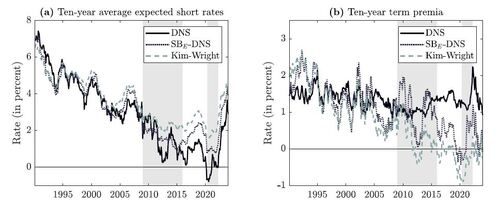
The left panel of Figure 7 shows the ten-year expected short-rate component, while the right panel shows the ten-year term premia. For comparison, we also include the estimates from Kim and Wright (2005) (KW) that are available from January 1990 onwards, explaining the shorter sample period in Figure 7. Before the GFC, the DNS and SB_E -DNS models produce rather similar decompositions with some slight differences in their level. In fact, the decompositions are also rather similar with the ones of KW. However, from the beginning of the ZLB period onward, the decompositions start to diverge between the models, where the DNS model produces a lower expected short rate and therefore overestimates the term premium compared to KW. The correlation between the term premium level (first difference) of DNS and KW is 0.408 (0.530). Meanwhile, the SB_E -DNS model produces expected short rates and term premia that are much closer to KW with a correlation of 0.930 for the term premium level and 0.905 for the term premium first differences. Hence, the SB_E -DNS model produces more plausible expected short-rate paths and term premia than the DNS model, especially during ZLB periods.

4 Conclusion

In this paper we develop a smooth shadow-rate version of the dynamic Nelson-Siegel (DNS) model to analyze and forecast U.S. government bond yields during the recent zero lower bound (ZLB) periods. Our smooth shadow-rate DNS model has a closed-form yield curve expression and hence can be easily estimated by means of (nonlinear) least squares. Consequently, it is straightforward to extend our model with time-varying parameters, macroeconomic variable integration or other variations of interest, which are not always possible in the no-arbitrage based and less tractable class of shadow-rate affine term structure models.

Our results indicate that our smooth shadow-rate DNS adaption dominates the original DNS approach and (shadow-rate) affine term structure models in terms of fitting and forecasting the yield curve for all forecast horizons, especially for short- and medium-term yields during ZLB periods. These forecast gains can be further improved by allowing for shifting endpoints in the yield dynamics, highlighting the relevance of accounting for long-run trends at the ZLB. Moreover, our model can be used to shape future policy expectations at the ZLB. This all can be produced at extremely low computational costs, making this approach highly applicable and attractive to practitioners and policy makers.

Acknowledgments

We are grateful to the editor, associate editor and two anonymous referees for their helpful comments and suggestions. We further would like to thank Michael Bauer, Dick van Dijk and Robin Lumsdaine for their insightful comments, as well as participants of the 15th International CFE Conference (2021, online), 4th International QFFE Conference (2022, Marseille), 9th IAAE Conference (2022, London), Econometric Society European Summer Meeting (2022, Milan), 5th Annual Workshop on Financial Econometrics (2022, Örebro), Annual AFA Meeting (2023, New Orleans) and seminar participants at Erasmus University Rotterdam (2021, online) and the University of Pennsylvania (2022, Philadelphia).

Disclosure statement

The authors report there are no competing interests to declare.

Table 1 Summary statistics of in-sample model fit

RMSE	Maturities (in months)					Total
	3	12	36	60	120
Panel A: Total period (August 1971 - December 2023)
DNS	12.4	8.0	6.6	9.0	11.3	7.2
B-DNS	12.3	8.0	6.6	9.0	11.3	7.2
SBG-DNS	11.7	7.4	6.0	7.8	10.0	6.6
SBS-DNS	11.5	7.3	6.0	7.5	9.5	6.4
SBE-DNS	11.5	7.3	6.0	7.3	9.2	6.3
AFNS	38.6	4.1	3.6	6.6	10.3	11.8
B-AFNS	36.8	4.4	4.4	6.7	10.2	11.4
Panel B: Pre-ZLB period (August 1971 - November 2008)
DNS	12.4	8.0	6.4	8.4	10.8	7.1
B-DNS	12.4	8.0	6.4	8.4	10.8	7.1
SBG-DNS	12.4	7.9	6.4	8.3	10.7	7.1
SBS-DNS	12.3	7.8	6.3	8.2	10.5	7.0
SBE-DNS	12.3	7.8	6.3	8.1	10.3	7.0
AFNS	40.9	4.4	3.9	6.9	11.1	12.5
B-AFNS	39.8	4.6	4.6	7.3	11.4	12.3
Panel C: ZLB period (December 2008 - December 2015)
DNS	13.9	8.5	7.4	14.0	17.2	9.2
B-DNS	13.7	8.4	7.2	13.9	17.0	9.1
SBG-DNS	9.0	4.1	3.2	8.3	10.5	5.6
SBS-DNS	7.7	3.1	3.4	6.3	7.8	4.4
SBE-DNS	6.9	2.9	3.4	5.5	6.3	3.9
AFNS	25.1	3.1	3.3	7.3	10.8	8.6
B-AFNS	14.7	3.0	3.6	6.3	7.7	5.8
Panel D: Post-ZLB period (January 2016 - December 2023)
DNS	10.5	7.4	6.7	5.3	5.5	5.3
B-DNS	10.4	7.4	6.7	5.3	5.5	5.3
SBG-DNS	10.4	7.2	6.2	4.4	4.8	4.9
SBS-DNS	10.6	7.2	6.2	4.3	4.8	4.9
SBE-DNS	10.8	7.2	6.2	4.3	4.8	5.0
AFNS	37.4	3.1	2.3	3.3	5.1	10.9
B-AFNS	36.1	4.6	4.1	3.9	4.9	10.8

Notes: This table contains the root mean squared fitting errors (in basis points) across maturities over four sample periods. We include the dynamic Nelson-Siegel (DNS) model, the shadow-rate DNS (B-DNS) model, the smooth shadow-rate DNS models with either the Gaussian-based approximation function (SB_G -DNS), the softplus approximation function (SB_S -DNS) or the inverse exponentially-based approximation function (SB_E -DNS), as well as the arbitrage-free Nelson-Siegel (AFNS) model with its shadow-rate counterpart (B-AFNS). All shadow-rate models are estimated with a fixed lower bound specification of $r_{LB}=0\%$.

Table 2 Relative out-of-sample performance compared to the DNS model

Horizons	$h=6 \mathbf{m}\mathbf{onths}$					$h=12 \mathbf{m}\mathbf{onths}$					$h=24 \mathbf{m}\mathbf{onths}$
Maturities	3	12	36	60	120	3	12	36	60	120	3	12	36	60	120
Panel A: Total period (August 1991 - December 2023)
RW	0.84***	0.79***	0.78***	0.81***	0.91**	0.91	0.86*	0.80**	0.81**	0.88**	1.03	1.01	0.90	0.86	0.88*
B-DNS ${ }^{\S }$	1.00	1.00	1.00	1.00	1.00	1.00	1.00	1.00	1.00	1.00	0.99	0.99	1.00	1.00	1.00
SBG-DNS	0.96***	0.98**	0.98**	1.00	1.00	0.97**	0.98*	0.99	1.00	1.00	0.97**	0.98**	0.99**	0.99	0.99
SBS-DNS	0.94***	0.96***	0.97**	0.98**	0.99	0.96**	0.97*	0.98	0.99	1.00	0.97*	0.97*	0.98**	0.99**	0.99
SBE-DNS	0.93***	0.94***	0.95***	0.97**	0.99	0.95**	0.95*	0.96*	0.98	1.00	0.96	0.96	0.96*	0.98*	0.99
AFNS	1.09**	1.03*	1.00	1.00	1.00	1.07*	1.03	1.02	1.03	1.03	1.05	1.03	1.05	1.07	1.10
B-AFNS	1.01	0.97	0.95***	0.95***	0.95***	1.01	0.98	0.96*	0.96**	0.95**	1.00	0.99	0.98	0.98	0.97
Panel B: Pre-ZLB period (August 1991 - November 2008)
RW	0.87*	0.80**	0.81**	0.83**	0.91	0.96	0.91	0.86	0.86	0.90	1.13*	1.12*	1.01	0.92	0.86*
B-DNS ${ }^{\S }$	1.00	1.00	1.00	1.00	1.00	1.00	1.00	1.00	1.00	1.00	1.00	1.00	1.00	1.00	1.00
SBG-DNS ${ }^{\S }$	1.00	1.00	1.00	1.00	1.00	1.00	1.00	1.00	1.00	1.00	1.00	1.00	1.00	1.00	1.00
SBS-DNS ${ }^{\S }$	0.98	0.99	0.99	0.99	1.00	0.99	0.99	0.99	1.00	1.00	1.00	1.00	1.00	1.00	1.00
SBE-DNS ${ }^{\S }$	0.97	0.97	0.98	0.99	0.99	0.99	0.99	0.99	0.99	0.99	1.00	1.00	1.00	1.00	1.00
AFNS	1.08**	1.02*	1.00	0.99	0.95*	1.04	1.02	1.00	1.00	0.96	1.01	1.00	1.02	1.04	1.02
B-AFNS	1.06**	1.01	0.98**	0.97***	0.94*	1.02	1.00	0.98**	0.97*	0.94*	1.00	0.99	0.99	0.99	0.94
Panel C: ZLB period (December 2008 - December 2015)
RW	0.39***	0.48***	0.46***	0.62***	0.86***	0.45***	0.43***	0.35***	0.47**	0.74***	0.80	0.73	0.57*	0.59*	0.72*
B-DNS ${ }^{\S }$	1.00	1.00	1.00	1.00	1.00	1.00	1.00	1.00	1.00	1.00	1.00	1.00	1.00	1.00	1.00
SBG-DNS	0.78***	0.82***	0.92***	0.98**	0.99	0.85***	0.89***	0.95***	0.99	1.01	0.94*	0.96*	0.99	1.01	1.02
SBS-DNS	0.69***	0.73***	0.84***	0.93***	0.99	0.76***	0.79**	0.89***	0.96*	1.02	0.88*	0.90*	0.96	1.00	1.04*
SBE-DNS	0.64***	0.67***	0.77***	0.88***	0.99	0.71***	0.72**	0.81**	0.91**	1.02	0.84*	0.85*	0.91*	0.96	1.05*
AFNS	1.40***	1.23***	1.03**	1.03**	1.12*	1.36***	1.22***	1.10***	1.11***	1.21**	1.27***	1.20***	1.15***	1.17***	1.27***
B-AFNS	0.86*	0.78***	0.78***	0.85***	0.93***	0.89*	0.83***	0.82***	0.87***	0.94**	0.95**	0.93***	0.94**	0.97	1.01
Panel D: Post-ZLB period (January 2016 - December 2023)
RW	0.96	0.88	0.95	0.96	0.95	1.00	0.96	1.02	1.01	0.99	1.06***	1.06***	1.08*	1.06	1.02
B-DNS ${ }^{\S }$	1.00	1.00	1.00	1.00	1.00	1.00	1.00	1.00	1.00	1.00	0.98	0.98	1.00	1.00	1.00
SBG-DNS	0.98	1.00	1.01	1.01	1.00	0.99	1.01*	1.02	1.01	0.99	0.96*	0.96*	0.96**	0.96**	0.95*
SBS-DNS	0.97	1.00	1.02	1.02	1.00	0.99	1.02	1.04	1.03	0.99	0.98***	0.98	0.97***	0.96***	0.94**
SBE-DNS	0.96	0.99	1.02	1.02	1.00	0.99	1.02	1.05	1.03	1.00	0.99	1.00	0.98	0.96***	0.94**
AFNS	0.88	0.93*	0.98	0.98	0.98	0.92	0.94	0.96	0.96	0.96	0.90	0.90	0.94	0.96	0.99
B-AFNS	0.97	0.98	1.02	1.01	0.97	1.04	1.04	1.06	1.04	0.98	1.05	1.03	1.02	1.00	0.95

Notes: This table contains the relative root mean squared forecast errors (RMSFEs) compared to the DNS model with AR(1) factor dynamics across maturities (in months) and forecast horizons (in months) over four evaluation periods. We include the shadow-rate DNS (B-DNS) model, the smooth shadow-rate DNS models with either the Gaussian-based approximation function (SB_G -DNS), the softplus approximation function (SB_S -DNS) or the inverse exponentially-based approximation function (SB_E -DNS), as well as the arbitrage-free Nelson-Siegel (AFNS) model with its shadow-rate counterpart (B-AFNS). All models have AR(1) factor dynamics. We consider expanding-window estimation with the initial sample from August 1971 to July 1991 (240 observations). All shadow-rate models are estimated with a fixed lower bound specification of $r_{LB}=0\%$. Shaded cells indicate that the respective model has a lower RMSFE than the DNS model (that is, a ratio smaller than one). The asterisks $*,**$, and $***$ indicate significant outperformance at the 10%, 5% and 1% level, respectively, based on the one-sided modified Diebold-Mariano test of Harvey et al. (1997). Note that the tests are not conducted for the B-DNS model in all periods and the SB-DNS models in the pre-ZLB period (as indicated with the $\S$ symbol), given that these models nest the DNS model for high yields and thus produce highly similar forecasts for a large part of the evaluation sample.

Table 3 Relative out-of-sample performance of different shifting-endpoint specifications compared to the baseline DNS model

Horizons		$h=6 \mathbf{m}\mathbf{onths}$					$h=12 \mathbf{m}\mathbf{onths}$					$h=24 \mathbf{m}\mathbf{onths}$
Maturities		3	12	36	60	120	3	12	36	60	120	3	12	36	60	120
Panel A: Total period (August 1991 - December 2023)
DNS	ESL	1.00	1.00	1.00	1.00	1.00	1.00	1.00	1.00	1.00	1.01	1.00	1.00	1.00	1.00	0.99
	ESLSC	0.91	0.90	0.85	0.86	0.95	0.96	0.93	0.87	0.86	0.92	1.06	1.03	0.92	0.88	0.89
	RZI	1.01	1.01	1.01	1.01	0.99	1.01	1.01	1.01	1.01	0.99	1.00	1.00	1.00	0.99	0.97
	RZIG	1.00	1.00	0.99	0.99	0.99	1.01	1.00	0.98	0.98	0.98	0.98	0.97	0.95	0.95	0.94
SB E-DNS	ESL	0.93***	0.95***	0.95***	0.97**	1.00	0.95**	0.96*	0.97*	0.98	1.01	0.97	0.97	0.96	0.97*	0.99
	ESLSC	0.87**	0.86**	0.84*	0.85	0.93*	0.94*	0.91*	0.86	0.86	0.91	1.06	1.03	0.93	0.89	0.88
	RZI	0.94***	0.95***	0.95***	0.97**	0.99	0.96**	0.96*	0.97*	0.98	0.99	0.97	0.96	0.96	0.97	0.97
	RZIG	0.96***	0.96***	0.94***	0.96**	0.99	0.97**	0.96*	0.95*	0.96	0.99	0.95*	0.94	0.92	0.93	0.95
Panel B: Pre-ZLB period (August 1991 - November 2008)
DNS	ESL	1.00	1.00	1.00	1.00	1.01	1.00	1.00	1.01	1.01	1.02	1.01	1.01	1.00	1.00	1.00
	ESLSC	0.95	0.92	0.88	0.88	0.95	1.02	0.99	0.93	0.91	0.95	1.16	1.16	1.05	0.97	0.91
	RZI	1.01	1.01	1.01	1.01	1.00	1.01	1.01	1.01	1.01	1.01	1.01	1.01	1.02	1.02	1.02
	RZIG	1.00	0.99	0.98	0.99	0.99	1.01	0.99	0.98	0.98	0.99	1.02	0.99	0.96	0.96	0.97
SBE-DNS	ESL ${ }^{\S }$	0.97	0.97	0.98	0.99	1.00	0.99	0.99	0.99	1.00	1.01	1.02	1.01	1.00	1.00	1.00
	ESLSC ${ }^{\S }$	0.93	0.90	0.87	0.87	0.94	1.01	0.98	0.92	0.90	0.94	1.16	1.16	1.05	0.97	0.90
	RZI ${ }^{\S }$	0.98	0.98	0.99	1.00	1.00	0.99	0.99	1.00	1.00	1.00	1.02	1.01	1.02	1.02	1.02
	RZIG ${ }^{\S }$	0.98	0.97	0.97	0.97	0.99	1.00	0.98	0.97	0.97	0.98	1.02	0.99	0.96	0.96	0.97
Panel C: ZLB period (December 2008 - December 2015)
DNS	ESL	1.00	1.00	1.00	1.00	0.99	1.00	1.00	1.00	1.00	0.99	1.00	1.00	1.00	0.99	0.98
	ESLSC	0.56	0.51	0.54	0.67	0.88	0.58	0.49	0.46	0.56	0.76	0.86	0.74	0.63	0.65	0.72
	RZI	1.02	1.01	1.01	1.00	0.97	1.02	1.01	1.01	1.01	0.96	1.02	1.02	1.01	1.00	0.97
	RZIG	0.86	0.90	0.96	0.97	0.96	0.85	0.89	0.95	0.96	0.94	0.86	0.90	0.94	0.95	0.93
SBE-DNS	ESL	0.65***	0.67***	0.77***	0.89***	0.99	0.72***	0.73**	0.82***	0.91***	1.02	0.84**	0.85**	0.91*	0.96 *	1.03
	ESLSC	0.49***	0.45***	0.49	0.63	0.82	0.53***	0.45**	0.42	0.52	0.72	0.85*	0.73	0.60	0.62	0.69**
	RZI	0.64***	0.67***	0.76***	0.87***	0.97	0.71***	0.72***	0.80***	0.89***	0.98	0.85***	0.86**	0.90**	0.94*	1.00**
	RZIG	0.61***	0.64***	0.75***	0.87***	0.97	0.65**	0.68**	0.79***	0.88***	0.98	0.75*	0.78*	0.86**	0.92*	0.98**
Panel D: Post-ZLB period (January 2016 - December 2023)
DNS	ESL	1.01	1.01	1.01	1.01	1.01	1.01	1.01	1.01	1.01	1.01	1.00	1.00	1.00	1.00	0.99
	ESLSC	0.98	1.00	1.05	1.04	1.01	1.01	1.03	1.06	1.05	1.02	1.04	1.06	1.05	1.03	1.00
	RZI	1.03	1.02	1.02	1.02	1.01	1.01	1.01	1.01	1.01	0.99	0.96	0.95	0.94	0.93	0.92
	RZIG	1.08	1.06	1.04	1.02	1.01	1.07	1.06	1.03	1.01	1.00	1.03	1.00	0.95	0.93	0.92
SBE-DNS	ESL	0.97	1.00	1.03	1.03	1.00	1.00	1.02	1.05*	1.04*	1.00	1.00	1.00	0.98	0.96	0.93*
	ESLSC	0.90	0.93*	1.02	1.03	0.99	0.97	1.00	1.08	1.08	1.03	1.07	1.08	1.09	1.07	1.00
	RZI	0.98	1.01	1.03	1.03	1.00	1.00	1.02	1.05*	1.04*	1.00	0.99***	0.99***	0.96***	0.94**	0.90
	RZIG	1.05	1.07	1.06	1.04	1.01	1.05	1.07	1.07**	1.05**	1.00	0.99	0.99*	0.96	0.93	0.89

Notes: This table contains the relative root mean squared forecast errors (RMSFEs) of the DNS model and smooth shadow-rate DNS model with the the inverse exponentially-based approximation function (SB_E -DNS) under different shifting-endpoint specifications compared to the baseline DNS model with AR(1) factor dynamics across maturities (in months) and forecast horizons (in months) over four evaluation periods. For both DNS and SB_E -DNS, we include the following shifting-endpoint specifications: (i) exponential smoothing for the level factor only (ESL), (ii) exponential smoothing for the level, slope and curvature factors (ESLSC), (iii) smoothed realized inflation for the level factor (RZI), (iv) RZI plus smoothed realized industrial production growth for the slope factor (RZIG). We consider expanding-window estimation with the initial sample from August 1971 to July 1991 (240 observations). All shadow-rate models are estimated with a fixed lower bound specification of $r_{LB}=0\%$. Shaded cells indicate that the respective model has a lower RMSFE than the baseline DNS model with AR(1) factor dynamics (that is, a ratio smaller than one). Bold numbers indicate that the smooth shadow-rate DNS model with the respective shifting-endpoint specifications outperforms the DNS model with the same shifting-endpoint specification, where the asterisks $*,**$, and $***$ indicate corresponding significant outperformance at the 10%, 5% and 1% level, respectively, based on the one-sided modified Diebold-Mariano test of Harvey et al. (1997). Note that the tests are not conducted for the SB_E -DNS models in the pre-ZLB period (as indicated with the $\S$ symbol), given that these models nest the DNS model for high yields and thus produce highly similar forecasts for a large part of the evaluation sample.

Figure 1 Illustration of the smooth approximations of the max function. Panel (a) shows the functions $f_G(x)=x\Phi (x)+\varphi (x),f_S(x)=\hspace{0.17em}\ln \hspace{0.17em}(1+e^x)$ and $f_E(x)=x/(1-e^{-x})$, while panel (b) shows the Gaussian-based approximation function $\gamma f_G(x/\gamma )$ for a range of values of γ.

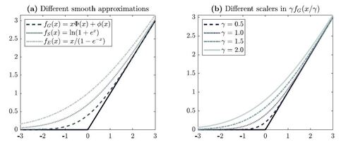
Figure 2 Time series of U.S. government bond yields (in percentage points) with shaded ZLB periods. Panel (a) shows the full sample-period, while panel (b) zooms in on the period after the Global Financial Crisis (GFC).

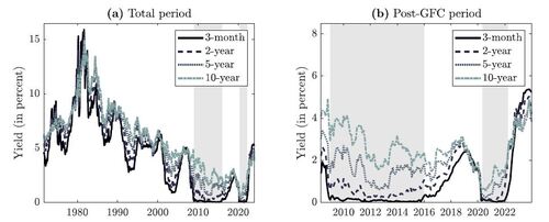
Figure 3 Estimated factors with their empirical proxies of the level (ten-year yield), slope (three-month minus ten-year yield), curvature (twice the two-year yield minus the sum of the three-month and ten-year yield), and short rate (three-month yield), as well as the differences between the estimated factors of the DNS model and its smooth shadow-rate versions based on the Gaussian-based approximation function (SB_G -DNS), the softplus approximation function (SB_S -DNS) and the inverse exponentially-based approximation function (SB_E -DNS), including shaded ZLB periods.

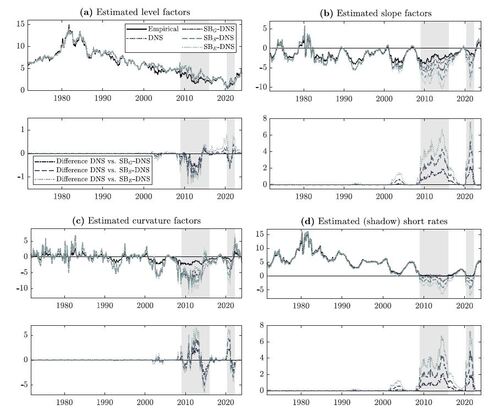
Figure 4 Conditional probabilities of negative three-month ahead yields based on $10,000$ simulations at each time t from the DNS model with shaded ZLB periods.

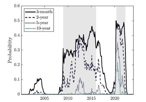
Figure 5 Three-month ahead realized and model-implied conditional volatility series of yields in the post-GFC period based on $10,000$ simulations at each time t from the DNS model and its (smooth) shadow-rate versions with shaded ZLB periods.

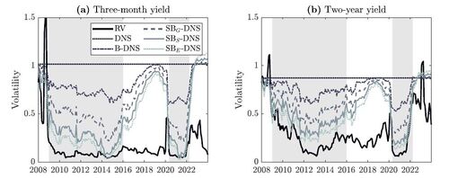
Figure 6 Shadow short-rate (SSR) and liftoff-horizon estimates in the post-GFC period. Panel (a) shows the SSR estimates from the smooth shadow-rate DNS models and from Wu and Xia (2016), while panel (b) shows the median liftoff-horizon estimates based on $10,000$ simulations at each time t from the smooth shadow-rate DNS models (including the interquartile range for SB_E -DNS), with shaded ZLB periods.

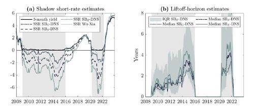
Figure 7 Ten-year average expected short-rate paths (panel a) and corresponding ten-year term premia (panel b) from the DNS model and SB_E -DNS model at each time t (based on $10,000$ simulations), as well as the corresponding estimates from Kim and Wright (2005), with shaded ZLB periods.