Estimating Latent-Variable Panel Data Models Using Parameter-Expanded SEM Methods

Abstract

This article presents new estimation algorithms for three types of dynamic panel data models with latent variables: factor models, discrete choice models, and persistent-transitory quantile processes. The new methods combine the parameter expansion (PX) ideas of Liu, Rubin, and Wu with the stochastic expectation-maximization (SEM) algorithm in likelihood and moment-based contexts. The goal is to facilitate convergence in models with a large space of latent variables by improving algorithmic efficiency. This is achieved by specifying expanded models within the M step. Effectively, we are proposing new estimators for the pseudo-data within iterations that take into account the fact that the model of interest is misspecified for draws based on parameter values far from the truth. We establish the asymptotic equivalence of the likelihood-based PX-SEM to an alternative SEM algorithm with a smaller expected fraction of missing information compared to the standard SEM based on the original model, implying a faster global convergence rate. Finally, in simulations we show that the new algorithms significantly improve the convergence speed relative to standard SEM algorithms, sometimes dramatically so, by reducing the total computing time from hours to a few minutes.

KEYWORDS:

• Algorithmic efficiency
• Discrete choice model
• Dynamic factor model
• Dynamic quantile model
• PX-EM
• Stochastic EM

1 Introduction

This article presents new estimation algorithms for dynamic panel data models with latent variables. Dynamic panel data models are widely used in applied work today. They tend to exhibit many latent variables over multiple periods (e.g., time-invariant, persistent, and transitory components), which are important to capture unobserved heterogeneity and dynamic responses (Arellano and Bonhomme 2017). However, the presence of latent variables brings challenges to the estimation.

Iterative methods like the stochastic expectation-maximization (SEM) algorithm can be useful tools for estimating models with latent variables (Diebolt and Celeux 1993).¹ Specifically, as a simulated version of the Expectation-Maximization (EM) algorithm (Dempster, Laird, and Rubin 1977), SEM iterates through an E-step where we draw latent variables from the posterior distribution of the model of interests given observables, and an M-step where we estimate the model as if the draws were observables until the parameters converge to the stationary distribution. It simplifies the estimation as it replaces the complex optimization problem, which involves multiple integrals due to latent variables, with a series of much simpler optimization problems under pseudo-complete data.

However, the slow convergence, an often voiced criticism of EM and its variants, tends to diminish its practical appeal. Indeed, the slow convergence issue in practice is even more pronounced: researchers often need to run the algorithms multiple times with different initial guesses and select the result based on criteria such as the likelihood value, to mitigate the negative effects of a “bad” initial guess and to address the possibility of the algorithm converging to a local maximum. Recent research has explored alternative samplers for latent variables when performing the E-step to improve sampling efficiency and stability.² In contrast, this article focuses on the potential improvement in the M-step.

In this article, we develop a new estimation method, the PX-SEM algorithm, by combining the parameter expansion ideas in Liu, Rubin, and Wu (1998) with the SEM algorithm. The goal is to facilitate convergence in models with a large space of latent variables by improving algorithmic efficiency. Even though the general concept of the PX-SEM algorithm applies to various models, we focus on three types of dynamic panel data models containing rich latent variable structures, where slow convergence issues are exacerbated, with the expectation that it can be particularly fruitful: (a) dynamic factor models, (b) random effects discrete choice models with persistent and transitory components, and (c) persistent-transitory dynamic quantile models with individual effects.³

The PX-SEM algorithm consists of two steps: an E-step, where we draw values of latent variables from the posterior distribution, and a PX-M-step, where we update parameters. Having the same E-step as the SEM algorithm, PX-SEM replaces the SEM M-step estimator with a more robust one, taking into account the possibility that E-step draws could violate model assumptions when parameter guesses are far from the true value. The PX-M step estimator is able to leverage additional information from the model itself, effectively “correcting” the M step updates in progressing to more accurate ones.

To implement the PX-SEM algorithm, one must construct an expanded model, the L model, which needs to satisfy two conditions. First, the L model must nest the original model, the O model. Second, there must exist a reduction function, a mapping from the L model parameters to the O model parameters, keeping the observed-data likelihood unchanged. After constructing a suitable L model, we can iterate between the E step and the PX-M step, which involves (a) estimating the L model and (b) mapping back to the O model parameters through the reduction function.

There are different ways to construct L models. All else being equal, a more flexible L model should improve the convergence rate. However, since our ultimate goal is to reduce the total computing time, we also need to consider the time spent in each iteration for estimating the L model and converting it to the O model. Therefore, taking these two factors into account, this article proposes a method to expand the model linearly. Linear expansion addresses the potential violation of zero-correlation assumptions.

In terms of statistical properties, Liu, Rubin, and Wu (1998) proves the monotone convergence of the parameter-expanded EM algorithm and its superior rate of convergence relative to its parent EM. By combining the results of Nielsen (2000) and Arellano and Bonhomme (2016), this article establishes the asymptotic equivalence of the likelihood-based PX-SEM to an alternative SEM algorithm with a smaller expected fraction of missing information compared to the standard O model based SEM, implying a faster global convergence rate and a smaller variance for the limiting stationary distribution. Finally, in the simulations, we show that PX-SEM can significantly improve algorithmic efficiency compared to the standard SEM algorithm, sometimes dramatically so. For example, in our numerical calculations for discrete choice and quantile models, SEM has still not converged even after running for 50–80 min whereas PX-SEM converges within 2–3 min.

This article belongs to an expanding literature that considers the application of the EM algorithm (Dempster, Laird, and Rubin 1977) and its variants in estimating latent variable models (Diebolt and Celeux 1993; Liu, Rubin, and Wu 1998; Arcidiacono and Jones 2003; Pastorello, Patilea, and Renault 2003; Arellano and Bonhomme 2016; Chen 2016; Arellano et al. 2023, among others). This article contributes to this literature in two ways. First, by developing a new estimation method, PX-SEM, which combines the parameter expansion idea with the SEM algorithm.⁴ The method offers appealing theoretical properties and the potential to enhance algorithmic efficiency, which is particularly valuable for complex models such as nonlinear panel data models, where SEM may encounter slow convergence issues. Second, the article proposes a specific class of linear expansions for implementing PX-SEM and develops new estimation algorithms for three types of latent-variable panel data models with enhanced algorithmic efficiency.

The article proceeds as follows. Section 2 illustrates the difference between the standard stochastic EM algorithm and the parameter-expanded stochastic EM algorithm using a simple toy model. In Section 3, a formal definition of PX-SEM is provided, along with a discussion of its statistical properties and implementation based on linear expansions. Sections 4–6 develop PX-SEM methods for three types of latent-variable panel data models: dynamic factor models, discrete choice models, and persistent-transitory dynamic quantile models, respectively. Finally, Section 7 concludes.

2 Toy Model

Based on a simple toy model, this section compares the parameter-expanded stochastic EM (PX-SEM) algorithm with the standard stochastic EM (SEM) algorithm and provides intuitions behind PX-SEM.

Consider the following model we want to estimate, denoted as the O model: $$y_i=y_i^{*}+{ϵ}_i,\text{ where }\left[\begin{array}{c}{y}_i^{*}\\ {ϵ}_i\end{array}\right]\stackrel{\text{iid}}{\sim }N(0,\left[\begin{array}{cc}{\sigma }^2& 0\\ 0& 1\end{array}\right]).\mathrm{\hspace{1em}}\mathrm{\hspace{1em}}(O\mathit{\text{Model}})$$

The observed outcomes are $y_1,\dots ,y_N$, and the latent variables whose distribution is of interest are $y_1^{*},\dots ,y_N^{*}$. The only unknown parameter is the standard deviation σ.

SEM

To implement the SEM algorithm, we need to start with an initial guess of the unknown parameter ${\widehat{\sigma }}^{(0)}$, and then iterate the following two steps for $s=0,1,\dots ,S$ until the convergence of ${\widehat{\sigma }}^{(s)}$ to the stationary distribution:

1. Stochastic E step: Draw $y_i^{*}$ from the posterior distribution $f_O(y_i^{*}|y_i;{\widehat{\sigma }}^{(s)})$

2. M step: Estimate the O model and update ${\widehat{\sigma }}^{(s+1)}$, that is ${\widehat{\sigma }}^{(s+1)}=\widehat{\text{std}}(y_i^{*})$ where $f_O(·)$ is the density function of O model. The final estimator is the average of the last S⁰ iterations $\widehat{\sigma }=\frac{1}{S^0}{\sum }_{S-S^0+1}^S{\widehat{\sigma }}^{(s)}$.

The nonstochastic version, the EM algorithm, is effective because it improves the observed-data likelihood in each iteration: (1) $$\begin{array}{c}\hspace{1em}\sum _i\hspace{0.17em}\mathrm{\text{log}}\hspace{0.17em}{f}_O(y_i;{\widehat{\sigma }}^{(s+1)})-\sum _i\hspace{0.17em}\mathrm{\text{log}}\hspace{0.17em}{f}_O(y_i;{\widehat{\sigma }}^{(s)})\\ \ge Q({\widehat{\sigma }}^{(s+1)}|{\widehat{\sigma }}^{(s)})-Q({\widehat{\sigma }}^{(s)}|{\widehat{\sigma }}^{(s)})\ge 0,\end{array}$$(1) where $Q({\widehat{\sigma }}^{(s+1)}|{\widehat{\sigma }}^{(s)})=\sum _i\int \hspace{0.17em}\mathrm{\text{log}}\hspace{0.17em}{f}_O(y_i,y_i^{*};{\widehat{\sigma }}^{(s+1)})f_O(y_i^{*}|y_i;{\widehat{\sigma }}^{(s)})d{y}_i^{*}$.⁵

PX-SEM

Now we introduce the PX-SEM algorithm. Like SEM, PX-SEM comprises an E step for draws of latent variables and an M step for updating parameters. While sharing the same E-step as SEM, PX-SEM’s M step involves (a) estimating an expanded model, the L model, and (b) mapping L model parameters to the O model parameters.

For this toy model, we propose the following L model:

$\begin{array}{c}{y}_i=y_i^{*}+{ϵ}_i,\\ \text{where }\left[\begin{array}{c}{y}_i^{*}\\ {ϵ}_i\end{array}\right]\stackrel{\text{iid}}{\sim }N(0,K\left[\begin{array}{cc}{\sigma }^2& 0\\ 0& 1\end{array}\right]K\prime ),\\ K=\left[\begin{array}{cc}k& 0\\ 1-k& 1\end{array}\right].\end{array}$ (L Model)

In addition to σ, the L model also contains an auxiliary parameter k. It is easy to verify that when k = 1, the two models coincide, that is $f_O(y_i^{*},y_i;\sigma )=f_L(y_i^{*},y_i;k=1,\sigma )$; and when $k\ne 1$, L model expands the O model by allowing for a nonzero correlation between $y_i^{*}$ and ϵ_i, as $\text{cov}(y_i^{*},{ϵ}_i)=k(1-k){\sigma }^2$. Moreover, the L model is unidentified with observables: for any L model with parameter values σ_L and k_L, the O model with parameter value $\sigma ={\sigma }_L$ has the same observed data likelihood, that is $f_O(y_i;{\sigma }_L)=f_L(y_i;{\sigma }_L,k_L)$.⁶

To implement PX-SEM, we begin with an initial guess of the unknown parameter ${\widehat{\sigma }}^{(0)}$, and then iterate the following two steps for $s=0,1,\dots ,S$ until the convergence of ${\widehat{\sigma }}^{(s)}$ to the stationary distribution:

1. Stochastic E step: Draw $y_i^{*}$ from the posterior distribution $f_O(y_i^{*}|y_i;{\widehat{\sigma }}^{(s)})$

2. PX-M step: Update parameters by

   1. Estimate the L model: ${\widehat{k}}_L=\frac{\widehat{\text{var}}(y_i^{*})}{\widehat{\text{cov}}(y_i^{*},y_i)},{\widehat{\sigma }}_L^{(s+1)}=\frac{\widehat{\text{std}}(y_i^{*})}{\left|{\widehat{k}}_L\right|}$

   2. Reduction: mapping from $({\widehat{\sigma }}_L^{(s+1)},{\widehat{k}}_L)$ to ${\widehat{\sigma }}^{(s+1)}$ maintaining the observed-data likelihood, that is $f_O(y_i;{\widehat{\sigma }}^{(s+1)})=f_L(y_i;{\widehat{\sigma }}_L^{(s+1)},{\widehat{k}}_L)$, and thus ${\widehat{\sigma }}^{(s+1)}={\widehat{\sigma }}_L^{(s+1)}$

The final estimator is the average of the last S⁰ iterations: $\widehat{\sigma }=\frac{1}{S^0}{\sum }_{S-S^0+1}^S{\widehat{\sigma }}^{(s)}$. As we see, the difference between the two methods lies in the estimators of the M step: the PX-SEM estimator is adjusted by $\frac{1}{\left|{\widehat{k}}_L\right|}$.

Figure 1 illustrates how PX-SEM has the potential to enhance algorithmic efficiency through the utilization of the auxiliary parameter k. Specifically, Figure 1(a) depicts a scatterplot of simulations generated by the data generating process (DGP), the O model with a true value of σ = 2. The X-axis and Y-axis display $y_i^{*}$ and ϵ_i, respectively, but only their sum $y_i=y_i^{*}+{ϵ}_i$ is used for estimation.

Fig. 1 Data and E-step draws under different guess values of σ.

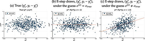
Figure 1(b) is the scatterplot of $(y_i^{*},y_i-y_i^{*})$ where $y_i^{*}$ is the E-step draws under the true value, that is $y_i^{*}\sim f_O(y_i^{*}|y_i;\sigma =2)$, and Figure 1(c) is the scatterplot of $(y_i^{*},y_i-y_i^{*})$ where $y_i^{*}$ is the E-step draws under an incorrect value σ = 1, that is $y_i^{*}\sim f_O(y_i^{*}|y_i;\sigma =1)$. Contrary to the case of Figure 1(b), where E-step draws are generated under correct guess, and there is no significant correlation between $y_i^{*}$ and $y_i-y_i^{*}$, Figure 1(c) presents a significant positive correlation between E-step draws $y_i^{*}$ and $y_i-y_i^{*}$, which is assumed to be zero by the O model. This “false” positive correlation arises because the draws are taken under a wrong condition that the variance of $y_i^{*}$ should not deviate significantly from one.

As a consequence, for the E-step draws in Figure 1(b), both M-step and PX-M step estimators are consistent: the SEM one is under a correct constraint k = 1. However, in the case of Figure 1(c), the M-step of SEM ignores the violation of the zero-correlation assumption at the current draws, while PX-SEM takes into account the “false” correlation by adding the parameter k. By construction, the extra flexibility induced by k leads to a better model fit of the PX-M step for the current draws and thus, a larger pseudo complete data likelihood. As we will show in Section 3, similar to EM, the PX-EM can improve observed-data likelihood in each iteration by transmitting gains from pseudo-complete data likelihood. Therefore, improving model fit as in the PX-M step essentially equates to improving the lower bound of the inequality in (1). Finally, by mapping the L model parameters to the O model parameters keeping the observed-data likelihood unchanged, we preserve the “gains” in likelihood. Intuitively, PX-SEM replaces the SEM M-step with a more robust estimator that leverages additional model information, namely, there is a linear correlation between the E-step draws $y_i^{*}$ and $y_i-y_i^{*}$, even though there should not be. Appendix A provides more explanation with illustrative figures.

Regarding the choice of the L model, there are many different ways of expanding the O model. Flexible expansion should help increase the convergence rate. Appendix A compares different L models and PX-M step estimators using the toy model. However, in practice, when we estimate more complex models, we must consider how easily we can estimate the L model and reduce it to the O model to avoid spending too much time in each iteration and increasing the total computing time. With this consideration in mind, we propose a linear expansion method in Session 3 and discuss its applications in Sessions 4–6.

As a final comment, the PX-SEM algorithm aims to enhance algorithm efficiency, even when E-step draws are appropriately obtained. For instance, as demonstrated in Appendix A, PX-SEM improves the convergence rate when the E-step draws are based on direct sampling. In more complex models where direct sampling is not feasible, and methods such as MCMC are required, the PX-SEM algorithm demonstrates lower sensitivity to poorly generated E-step draws. This can be justified if one of the ways that “bad” draws manifest themselves is through violations of model assumptions. Moreover, an MCMC-based E-step generally requires more time for each iteration, so reducing the iterations needed for convergence can significantly reduce the total computing time. For example, as shown in Sections 5 and 6, while SEM can take more than 3000 sec without showing signs of convergence, PX-SEM converges within a couple of minutes.

3 Parameter Expanded Stochastic EM Algorithm

The section begins by defining the PX-SEM algorithm. Following that, we discuss its statistical properties and explore the reasons behind its potential to enhance algorithmic efficiency. Specifically, we establish the asymptotic equivalence between PX-SEM and an alternative SEM with a reduced expected fraction of missing information. Finally, we propose a general approach, the linear expansion method, for the implementation.

3.1 Definition of PX-SEM Algorithm

Setup

Let $\{Y_i,X_i,Y_i^{*}\}$ for $i=1,\dots ,N$ be iid random variables following the distribution of the O model, denoted as $f_O(Y_i|X_i;\theta )={\int }_{Y_i^{*}}{f}_O(Y_i,Y_i^{*}|X_i;\theta )d{Y}_i^{*}$. Here $W_i\equiv [Y_i^{\prime }{X}_i^{\prime }]\prime$ represents the observable vector, $Y_i^{*}$ is the latent-variable vector, and θ is the unknown parameter vector to be estimated. The true value, $\overline{\theta }$, satisfies the equation $E({\Psi }_O(Y_i^{*},W_i;\overline{\theta }))=0$, where ${\Psi }_O(·)$ represents the score function of the complete O model in the case of the likelihood-based PX-SEM algorithm and moment restrictions in the case of the moment-based one. The law of iterated expectations implies that the true value $\overline{\theta }$ also satisfies the equation: (2) $$E(\int {\Psi }_O(Y_i^{*},W_i;\overline{\theta })f_O(Y_i^{*}|W_i;\overline{\theta })d{Y}_i^{*})=0.$$(2)

Define $\widehat{\theta }$ as the solution of the integrated moment restrictions of the original O model, $\sum _i(\int {\Psi }_O(Y_i^{*},W_i;\widehat{\theta })f_O(Y_i^{*}|W_i;\widehat{\theta })d{Y}_i^{*})=0$, a sample analogy to (2). In the case of a likelihood-based algorithm, we know that $\widehat{\theta }$ is the MLE.

Denote the expanded model, the L model, as $f_L(Y_i|X_i;\theta ,K)={\int }_{Y_i^{*}}{f}_L(Y_i,Y_i^{*}|X_i;\theta ,K)d{Y}_i^{*}$, where K represents the auxiliary parameter vector. The expanded L model needs to satisfy two conditions: (a) The L model nests the O model: There exists K = K₀ such that $f_O(Y_i,Y_i^{*}|X_i;\theta )=f_L(Y_i,Y_i^{*}|X_i;\theta ,K_0),\forall \theta$, and (b) Existence of reduction function: There exists a mapping from the L model parameters to the O model parameters, the reduction function $\theta =R({\theta }_L,K)$, such that the observed-data likelihood is preserved: $f_O(Y_i|X_i;R({\theta }_L,K))=f_L(Y_i|X_i;{\theta }_L,K),\forall {\theta }_L,K$.

Let ${\Psi }_L^{\theta }(·)$ denote the score function of the L model with respect to θ in the case of the likelihood-based PX-SEM algorithm and the same moment restrictions as ${\Psi }_O(·)$ in the case of the moment-based one. Under condition (a), we have ${\Psi }_L^{\theta }(Y_i^{*},W_i;\theta ,K_0)={\Psi }_O(Y_i^{*},W_i;\theta )$, and thus $E({\Psi }_L^{\theta }(Y_i^{*},W_i;\overline{\theta },K_0))=0$. Additionally, assuming that K is identified when we observe $Y_i^{*}$, meaning that there exists ${\Psi }_L^K(·)$ such that $E({\Psi }_L^K(Y_i^{*},W_i;\overline{\theta },K_0))=0$, we then have $E({\Psi }_L(Y_i^{*},W_i;\overline{\theta },K_0))=0$, where ${\Psi }_L(·)=[{\Psi }_L^{\theta }(·)\prime {\Psi }_L^K(·)\prime ]\prime$. By the law of iterated expectations, this implies:⁷ (3) $$E(\int {\Psi }_L(Y_i^{*},W_i;\overline{\theta },K_0)f_O(Y_i^{*}|W_i;R(\overline{\theta },K_0))d{Y}_i^{*})=0.$$(3)

Definition of the PX-SEM algorithm

Before we outline the general steps of PX-SEM, let us take a look at the SEM algorithm for comparison. SEM is an iterative algorithm where, in the E step, we make draws of latent variables $Y_i^{*}$ from the posterior distribution $f_O(Y_i^{*}|W_i;{\widehat{\theta }}^{(s)})$ under the parameter guess ${\widehat{\theta }}^{(s)}$, and in the M step, we update it to ${\widehat{\theta }}^{(s+1)}$, which satisfies $\sum _i{\Psi }_O(Y_i^{*},W_i;{\widehat{\theta }}^{(s+1)})=0$. This stochastic version differs from the original EM algorithm as it replaces the integral in (2) with latent draws.

In contrast, the PX-SEM algorithm proposes iterations that are better linked to (3): while we still make draws of latent variables $Y_i^{*}$ from the posterior distribution $f_O(Y_i^{*}|W_i;{\widehat{\theta }}^{(s)})$ under the parameter guess ${\widehat{\theta }}^{(s)}$, we use the expanded model to update the parameter to ${\widehat{\theta }}^{(s+1)}$, satisfying ${\widehat{\theta }}^{(s+1)}=R({\widehat{\theta }}_L,\widehat{K})$, where $\sum _i{\Psi }_L(Y_i^{*},W_i;{\widehat{\theta }}_L,\widehat{K})=0$.

The general steps are as follows: starting with an initial guess ${\widehat{\theta }}^{(0)}$, we iterate the following two steps for $s=0,1,2,\dots ,S$ until ${\widehat{\theta }}^{(s)}$ converges to the stationary distribution:

1. Stochastic E step: Draw $Y_i^{*}$ from the posterior distribution $f_O(Y_i^{*}|W_i;{\widehat{\theta }}^{(s)})$

2. PX-M step: Update parameters by

   1. Estimate L model: $\sum _i{\Psi }_L(Y_i^{*},W_i;{\widehat{\theta }}_L,\widehat{K})=0$

   2. Reduction: ${\widehat{\theta }}^{(s+1)}=R({\widehat{\theta }}_L,\widehat{K})$ subject to $f_O(Y_i|X_i;{\widehat{\theta }}^{(s+1)})=f_L(Y_i|X_i;{\widehat{\theta }}_L,\widehat{K})$

Reduction function

In practice, one of the challenges in implementing the PX-SEM algorithm is to find the reduction function associated with the L model. However, if we construct the L model such that the auxiliary parameter K does not affect the observed-data likelihood, that is $f_O(Y_i|X_i;{\theta }_L)=f_L(Y_i|X_i;{\theta }_L,K)$, then immediately, the reduction function becomes $R(\theta ,K)=\theta$. As a result, PX-SEM can be simplified as follows:

1. Stochastic E step: Draw $Y_i^{*}$ from the posterior distribution $f_O(Y_i^{*}|W_i;{\widehat{\theta }}^{(s)})$

2. PX-M step: Update parameters by solving $\sum _i{\Psi }_L(Y_i^{*},W_i;{\widehat{\theta }}^{(s+1)},\widehat{K})=0$

Comparing the PX-M and M steps, we find that the M-step estimator is a constrained version of the PX-M-step estimator with the constraint K = K₀. Intuitively, when the E-step draws $Y_i^{*}$ are generated under a guess ${\widehat{\theta }}^{(s)}$ close enough to the true value, the M-step estimator is under the correct restriction, leading both the M-step and PX-M-step estimators to be consistent at that iteration, as indicated by (2) and (3).

However, when the guess ${\widehat{\theta }}^{(s)}$ deviates significantly from the true value, causing the draws $Y_i^{*}$ to violate certain model assumptions, we would expect the PX-SEM estimator to exhibit greater “robustness” due to extra flexibility brought by auxiliary parameter K. As shown in the following section, the likelihood-based PX-M step can achieve a larger pseudo-complete data likelihood improvement, which could further lead to a greater observed-data likelihood improvement compared to the M step.

3.2 Statistical Properties

This section focuses on the statistical properties of likelihood-based algorithms. We will first show that the parameter-expanded EM algorithm exhibits nonnegative improvement in the observed-data log-likelihood at each iteration. Next, for the stochastic version, PX-SEM, we will establish its asymptotic equivalence to an alternative SEM algorithm with a smaller expected fraction of missing information compared to the standard O model based SEM, which implies a faster global convergence rate and a smaller variance for the limiting stationary distribution in a semipositive definite order.

Convergence

Following Liu, Rubin, and Wu (1998), we now prove that PX-EM algorithm increases the observed-data likelihood in each iteration. The change in the observed-data log-likelihood between iterations $\sum _i\hspace{0.17em}\mathrm{\text{log}}\hspace{0.17em}{f}_O(Y_i|X_i;{\widehat{\theta }}^{(s+1)})-\sum _i\hspace{0.17em}\mathrm{\text{log}}\hspace{0.17em}{f}_O(Y_i|X_i;{\widehat{\theta }}^{(s)})$ equals $$\begin{array}{c}\sum _i\hspace{0.17em}\mathrm{\text{log}}\hspace{0.17em}{f}_L(Y_i|X_i;{\widehat{\theta }}_L,\widehat{K})\text{ ‐}\sum _i\hspace{0.17em}\mathrm{\text{log}}\hspace{0.17em}{f}_L(Y_i|X_i;{\widehat{\theta }}^{(s)},K_0)\\ \ge Q({\widehat{\theta }}_L,\widehat{K}|{\widehat{\theta }}^{(s)},K_0)\text{ ‐ }Q({\widehat{\theta }}^{(s)},K_0|{\widehat{\theta }}^{(s)},K_0)\ge 0,\end{array}$$where $Q({\widehat{\theta }}_L,\widehat{K}|{\widehat{\theta }}^{(s)},K_0)=\sum _i\int \hspace{0.17em}\mathrm{\text{log}}\hspace{0.17em}{f}_L(Y_i,Y_i^{*}|X_i;{\widehat{\theta }}_L,\widehat{K})f_L(Y_i^{*}|W_i;{\widehat{\theta }}^{(s)},K_0)d{Y}_i^{*}$.

The equality holds because of both condition (a): When K = K₀, two models coincide, meaning $f_O(Y_i|X_i;{\widehat{\theta }}^{(s)})=f_L(Y_i|X_i;{\widehat{\theta }}^{(s)},K_0)$, and condition (b): The reduction function exists, and thus by construction $f_O(Y_i|X_i;{\widehat{\theta }}^{(s+1)})=f_L(Y_i|X_i;{\widehat{\theta }}_L,\widehat{K})$. We then apply Gibbs’ inequality. Finally, the definition of ${\widehat{\theta }}_L$, which is ${\widehat{\theta }}_L,\widehat{K}\equiv \mathrm{\text{arg}}{\mathrm{\text{max}}}_{\theta ,K}Q(\theta ,K|{\widehat{\theta }}^{(s)},K_0)$, leads to a nonnegative change in observed-data likelihood. Notably, the result also implies that $(\widehat{\theta },K_0)$ is a fixed point of PX-EM, where $\widehat{\theta }$ represents the MLE.⁸

As a final remark, the L model nesting the O model implies the following inequality: $$\begin{array}{c}Q({\widehat{\theta }}_L,\widehat{K}|{\widehat{\theta }}^{(s)},K_0)-Q({\widehat{\theta }}^{(s)},K_0|{\widehat{\theta }}^{(s)},K_0)\\ \ge Q({\widehat{\theta }}_{\mathit{\text{EM}}}^{(s+1)},K_0|{\widehat{\theta }}^{(s)},K_0)-Q({\widehat{\theta }}^{(s)},K_0|{\widehat{\theta }}^{(s)},K_0),\end{array}$$where ${\widehat{\theta }}_{\mathit{\text{EM}}}^{(s)}=\mathrm{\text{arg}}{\mathrm{\text{max}}}_{\theta }\sum _i\int \hspace{0.17em}\mathrm{\text{log}}\hspace{0.17em}{f}_O(Y_i,Y_i^{*}|X_i;\theta )f_L(Y_i^{*}|W_i;{\widehat{\theta }}^{(s)},K_0)d{Y}_i^{*}$. Therefore, the parameter expansion technique can be intuitively interpreted as a way to improve the lower bound of the log-likelihood increment compared to the EM algorithm.

Asymptotic properties

We first characterize the dynamics of PX-SEM updates. Define Θ as the joint set of auxiliary and O model parameters, $\Theta \equiv [\theta ;K]$. Accordingly, $\overline{\Theta }\equiv [\overline{\theta };K_0]$ represents the vector of true values, and $\widehat{\Theta }\equiv [\widehat{\theta };K_0]$ represents the MLE of the O model. Given any estimate ${\widehat{\Theta }}^{(s)}=[{\widehat{\theta }}^{(s)};K_0]$ in the iteration s, PX-SEM generates the next update from a Markov process: $\sum _i{\Psi }_L(Y_i^{*},W_i;{\widehat{\Theta }}^{(s+1)})=0$, where $Y_i^{*}\sim f_L(Y_i^{*}|W_i;{\widehat{\Theta }}^{(s)})$.⁹¹⁰ Expanding around $\widehat{\Theta }$ and considering $\widehat{\theta }\underset{}{\overset{p}{\to }}\overline{\theta }$, as shown in detail in Appendix B, we have (4) $$\begin{array}{c}({\widehat{\Theta }}^{(s+1)}-\widehat{\Theta })=(I-A^{-1}V)({\widehat{\Theta }}^{(s)}-\widehat{\Theta })+A^{-1}{ϵ}^{(s)}\\ \hspace{1em}+o_p(N^{-(1/2)}),\end{array}$$(4) where, under the correct specification, $A=E({\Psi }_L(Y_i^{*},W_i;\overline{\Theta }){\Psi }_L(Y_i^{*},W_i;\overline{\Theta })\prime )$ is the L model-based complete-data information matrix, $V=E({\Psi }_L(W_i;\overline{\Theta }){\Psi }_L(W_i;\overline{\Theta })\prime )$ is the L model-based observed-data information matrix, $I-A^{-1}V$ is the expected fraction of missing information, and $\sqrt{N}{ϵ}^{(s)}\underset{}{\overset{d}{\to }}\mathcal{N}(\stackrel{\rightharpoonup }{0},A-V)$.

The SEM iterations can be characterized in the same way: (5) $$\begin{array}{c}({\widehat{\theta }}_{\mathit{\text{SEM}}}^{(s+1)}-\widehat{\theta })=(I-A_{\theta \theta }^{-1}{V}_{\theta \theta })({\widehat{\theta }}_{\mathit{\text{SEM}}}^{(s)}-\widehat{\theta })\\ \hspace{1em}+A_{\theta \theta }^{-1}{ϵ}_{\theta }^{(s)}+o_p(N^{-(1/2)}),\end{array}$$(5) where $A_{\theta \theta }$ represents the O model-based complete-data information matrix, $V_{\theta \theta }$ represents the O model-based observed-data information matrix, $F_{\mathit{\text{SEM}}}\equiv I-A_{\theta \theta }^{-1}{V}_{\theta \theta }$ is the expected fraction of missing information, and $\sqrt{N}{ϵ}_{\theta }^{(s)}\underset{}{\overset{d}{\to }}\mathcal{N}(\stackrel{\rightharpoonup }{0},A_{\theta \theta }-V_{\theta \theta })$. Moreover, PX-SEM and SEM dynamics are closely connected: $$A=\left[\begin{array}{cc}{A}_{\theta \theta }& A_{\theta K}\\ A_{K\theta }& A_{\mathit{\text{KK}}}\end{array}\right],V=\left[\begin{array}{cc}{V}_{\theta \theta }& 0\\ 0& 0\end{array}\right],$$ where $A_{\theta K}\equiv -\frac{\partial }{\partial K\prime }{|}_{\overline{\Theta }}E({\tilde{\Psi }}_L^{\theta }(Y_i^{*},W_i;\Theta ))$ and $A_{\mathit{\text{KK}}}\equiv -\frac{\partial }{\partial K\prime }{|}_{\overline{\Theta }}E({\tilde{\Psi }}_L^K(Y_i^{*},W_i;\Theta ))$.

We now present the main results of the asymptotic properties, building on Liu, Rubin, and Wu (1998) and Nielsen (2000), with detailed discussions provided in Appendix B.

Theorem 1.

The PX-SEM iteration of ${\widehat{\theta }}^{(s)}$ is asymptotically equivalent to SEM iteration with observed-data information matrix $V_{\theta \theta }$ and complete-data information matrix $A_{\theta \theta }-A_{\theta K}{A}_{\mathit{\text{KK}}}^{-1}{A}_{K\theta }$.

Proof.

Let H denote the inverse of matrix A, that is $$H=\left[\begin{array}{cc}{H}_{\theta \theta }& H_{\theta K}\\ H_{K\theta }& H_{\mathit{\text{KK}}}\end{array}\right]\equiv {\left[\begin{array}{cc}{A}_{\theta \theta }& A_{\theta K}\\ A_{K\theta }& A_{\mathit{\text{KK}}}\end{array}\right]}^{-1}=A^{-1},$$where, by design, $H_{\theta \theta }^{-1}=A_{\theta \theta }-A_{\theta K}{A}_{\mathit{\text{KK}}}^{-1}{A}_{K\theta }$. Then the coefficient matrix $I-A^{-1}V$ and the asymptotic variance of the innovation term $A^{-1}{ϵ}^{(s)}$ in (4) become: $$\begin{array}{c}I-A^{-1}V=\left[\begin{array}{cc}I-H_{\theta \theta }{V}_{\theta \theta }& 0\\ -H_{K\theta }{V}_{\theta \theta }& I\end{array}\right],\\ A^{-1}(A-V)A^{-1}\\ =\left[\begin{array}{cc}{H}_{\theta \theta }(H_{\theta \theta }^{-1}-V_{\theta \theta })H_{\theta \theta }& H_{\theta K}-H_{\theta \theta }{V}_{\theta \theta }{H}_{\theta K}\\ H_{K\theta }-H_{K\theta }{V}_{\theta \theta }{H}_{\theta \theta }& H_{\mathit{\text{KK}}}-H_{K\theta }{V}_{\theta \theta }{H}_{\theta K}\end{array}\right].\end{array}$$

It becomes evident that the PX-SEM process of ${\widehat{\theta }}^{(s+1)}$ is asymptotically equivalent to an alternative SEM dynamics, described by (6), which shares the same observed-data information matrix $V_{\theta \theta }$ as the standard SEM in (5), but replaces the original complete-data information matrix $A_{\theta \theta }$ by $H_{\theta \theta }^{-1}=A_{\theta \theta }-A_{\theta K}{A}_{\mathit{\text{KK}}}^{-1}{A}_{K\theta }$. (6) $$\begin{array}{c}({\widehat{\theta }}^{(s+1)}-\widehat{\theta })=(I-H_{\theta \theta }{V}_{\theta \theta })({\widehat{\theta }}^{(s)}-\widehat{\theta })\\ +H_{\theta \theta }{\widetilde{ϵ}}_{\theta }^{(s)}+o_p(N^{-(1/2)}),\end{array}$$(6)

where $\sqrt{N}{\widetilde{ϵ}}_{\theta }^{(s)}\underset{}{\overset{d}{\to }}\mathcal{N}(\stackrel{\rightharpoonup }{0},H_{\theta \theta }^{-1}-V_{\theta \theta })$, and $F_{\mathit{\text{PX}}}\equiv I-H_{\theta \theta }{V}_{\theta \theta }$ is the expected fraction of missing information.¹¹□

Since $H_{\theta \theta }=A_{\theta \theta }^{-1}+H_{\theta K}{H}_{\mathit{\text{KK}}}^{-1}{H}_{K\theta }$, under the condition that A is positive definite, $H_{\theta \theta }\ge A_{\theta \theta }^{-1}$ in a semipositive definite order, implying the largest eigenvalue of F_PX is no greater than the largest eigenvalue of F_SEM. Applying Theorem 1, this comparison in the expected fraction of missing information matrix between PX-SEM and SEM immediately implies the dominance of PX-SEM in convergence rate, as stated in Corollary 1.

Corollary 1.

PX-SEM dominates SEM in global rate of convergence.

Proof.

In Appendix B.2. □

Moreover, Nielsen (2000) provides conditions under which the SEM update is ergodic and characterizes the limiting stationary distribution, based on which Corollary 2 describes the limiting stationary distribution of PX-SEM and compares it with SEM.¹²

Corollary 2.

The limiting stationary distribution of PX-SEM updates ${\widehat{\theta }}^{(s)}$, conditional on W_i, is $\sqrt{N}({\widehat{\theta }}^{(s)}-\widehat{\theta })\underset{}{\overset{d}{\to }}\mathcal{N}(0,V_{\theta \theta }^{-1}(I-{(I+F{\prime }_{\mathit{\text{PX}}})}^{-1}))$, and unconditionally, is $\sqrt{N}({\widehat{\theta }}^{(s)}-\overline{\theta })\underset{}{\overset{d}{\to }}\mathcal{N}(0,V_{\theta \theta }^{-1}(2I-{(I+F{\prime }_{\mathit{\text{PX}}})}^{-1}))$, with its variances being less than or equal to those of the standard O model-based SEM, that is, $V_{\theta \theta }^{-1}(2I-{(I+F{\prime }_{\mathit{\text{PX}}})}^{-1})-V_{\theta \theta }^{-1}(2I-{(I+F{\prime }_{\mathit{\text{SEM}}})}^{-1})=V_{\theta \theta }^{-1}(I-{(I+F{\prime }_{\mathit{\text{PX}}})}^{-1})-V_{\theta \theta }^{-1}(I-{(I+F{\prime }_{\mathit{\text{SEM}}})}^{-1})\le 0$ in semipositive definite order.

Proof.

In Appendix B.2. □

Corollary 2 implies that PX-SEM updates exhibit smaller fluctuation along iterations in large samples. Moreover, since the final estimator is the average of the last S⁰ iterations after convergence, $\widehat{\theta }=\frac{1}{S^0}{\sum }_{S-S^0+1}^S{\widehat{\theta }}^{(s)}$, which converges to the MLE as the number of iterations increases, PX-SEM and SEM estimators share the same asymptotic variance.¹³

When the M-step is moment-based, in general, convergence is not guaranteed. Under convergence, the speed does not necessarily dominate SEM. Indeed, Appendix A shows an example where moment-based PX-SEM underperforms SEM for some initial guesses.

However, moment-based PX-SEM may be the preferred choice in practice for at least two crucial reasons. First, in some cases, obtaining GMM estimators is much easier, such as in the quantile model discussed in Section 6. Since our final target is to reduce the computing time, we should consider not only the number of iterations but also the time spent in each iteration. Second, even if obtaining the MLE of the O model is feasible, restricting ourselves to a tractable MLE in the PX-M step can limit the flexibility in building the L model, negatively impacting the convergence rate. Appendix A shows an example of the toy model where the moment-based PX-SEM with a more flexible L model outperforms the likelihood-based PX-SEM, which uses a less flexible L model.

3.3 Implementation based on Linear Expansions

So far, we have shown that a new estimation method, PX-SEM, which combines the parameter expansion technique with the SEM algorithm, has attractive theoretical properties relative to ordinary SEM and the potential to achieve large computational gains.

However, the parameter expansion technique itself does not speak of the selection of the L model. On the one hand, all else being equal, a more flexible L model should improve the convergence rate. On the other hand, we also need to consider the time spent in each iteration to estimate the L model and convert it to the O model since our ultimate goal is to reduce the total computing time. Therefore, another contribution of this article is to propose a specific class of linear expansions, targeting the potential violation of zero-correlation assumptions, which can be generally applied to a wide range of models.

Considering an O model of the form: $Y_i=G(Y_i^{*};\theta ),Y_i^{*}\sim F_O(\theta )$, where both $G(·)$ and $F_O(·)$ are known parametric functions up to unknown parameter θ, we propose the following linear expansion to $Y_i^{*}$¹⁴

$\begin{array}{c}{Y}_i=G(Y_i^{*};\theta ),Y_i^{*}=A{Y}_i^{†},Y_i^{†}\sim F_O(\theta ),\\ \mathrm{s}.\mathrm{t}.G(Y_i^{*};\theta )\stackrel{d}{=} G(Y_i^{†};\theta )(\mathit{\text{equally distributed}}),\end{array}$ (L Model)where the auxiliary parameter is given by $K=\text{vec}(A)$.¹⁵

The expansion is straightforward. We assume that the latent variable $Y_i^{†}$ follows the same distribution as the O model counterpart. However, the E-step draws $Y_i^{*}$, which directly contribute to the measurement equation and observable Y_i, result from an affine transformation applied to $Y_i^{†}$. It is easy to check that when A = I, the L model coincides with the O model, whereas when $A\ne I$, it allows us to introduce linear correlations among elements of $Y_i^{*}$. The constraint ensures that the auxiliary parameters do not affect the observed-data likelihood, simplifying the reduction function to $R(\theta ,K)=\theta$.¹⁶

To implement the PX-SEM algorithm, in the E-step, we draw $Y_i^{*}$ from the O model based posterior distribution as discussed before. In the PX-M step, we leverage moment constraints or the distribution of $F_O(\theta )$ to pin down A and θ.

This method has the advantage that, despite the model of interest being nonlinear, the expansion is linear in latent variables, which are drawn from the E-step and treated as observables in the PX-M step. Thus, we can identify the auxiliary parameters separately through a relatively simple linear model, regardless of the specific form of $G(·)$.

In the following sections, we discuss three applications: (a) dynamic factor models, (b) discrete choice models, and (c) quantile models, for which we propose PX-SEM algorithms based on linearly expanded models.

4 Dynamic Factor Models

The first type of model we discuss is the dynamic factor model (Geweke 1977). The appeal of this class of models is their ability to explain variation across multiple dimensions using fewer latent common factors. Applications span multiple fields, including topics in macroeconomics and finance, among others (Bai and Ng 2008; Stock and Watson 2006, 2011). While we will focus on a specific single-factor O model, it is worth noting that the same approach for implementing the PX-SEM algorithm can be applied to models with multiple latent factors. The O model to be estimated is as follows:

$y_{\mathit{\text{it}}}={\lambda }_i{\nu }_t+{ϵ}_{\mathit{\text{it}}}\text{ and }{\nu }_t={\nu }_{t-1}+u_t,$ (O Model)where ${ϵ}_{\mathit{\text{it}}}\stackrel{\text{iid}}{\sim }N(0,{\sigma }_i^2),u_t\stackrel{\text{iid}}{\sim }N(0,1),{\nu }_0=0$, and u_t is independent of ϵ_it.

The model contains a latent common factor ν_t that follows a Gaussian random walk. We observe N different measures, y_i, where $i=1,\dots ,N$, over a total of T periods, with each measure associated with a distinct factor loading λ_i. The set of unknown parameters is denoted as $\theta \equiv ({\lambda }_1,\dots ,{\lambda }_N,{\sigma }_1,\dots ,{\sigma }_N)$.¹⁷

SEM

We first explain the SEM procedure. Let $\nu \equiv [{\nu }_1{\nu }_2\dots {\nu }_T]\prime$. Starting with an initial guess ${\widehat{\theta }}^{(0)}$, we iterate through the E-step and the M-step for $s=0,1,2,\dots ,S$ until the convergence of ${\widehat{\theta }}^{(s)}$ to the stationary distribution:

1. Stochastic E step: Draw ν from the posterior distribution $f_O(\nu |y_i;{\widehat{\theta }}^{(s)})$

2. M step: Update ${\widehat{\theta }}^{(s+1)}=({\widehat{\lambda }}_1,\dots ,{\widehat{\lambda }}_N,{\widehat{\sigma }}_1,\dots ,{\widehat{\sigma }}_N)$ $${\widehat{\lambda }}_i={(\sum _t{\nu }_t^2)}^{-1}(\sum _t{\nu }_t{y}_{\mathit{\text{it}}})\text{ and }{\widehat{\sigma }}_i=\widehat{\text{std}}(y_{\mathit{\text{it}}}-{\widehat{\lambda }}_i{\nu }_i),\forall i$$

PX-SEM

To implement PX-SEM, we construct a simple L model as follows:

$y_{\mathit{\text{it}}}={\lambda }_i{\nu }_t+{ϵ}_{\mathit{\text{it}}}\text{ and }{\nu }_t={\nu }_{t-1}+u_t,$ (L Model)where ${ϵ}_{\mathit{\text{it}}}\stackrel{\text{iid}}{\sim }N(0,{\sigma }_i^2),u_t\stackrel{\text{iid}}{\sim }N(0,k^2),{\nu }_0=0$, and u_t is independent of ϵ_it.

This L model expands the O model by introducing an auxiliary parameter, k, allowing the variance of the persistent shock u_t to deviate from 1. Since k can always take the value of 1, making the two models coincide, the L model satisfies condition (a). Moreover, it is easy to verify that reduction function $R({\lambda }_1,\dots ,{\lambda }_N,{\sigma }_1,\dots ,{\sigma }_N,k)=({\lambda }_{1}k,\dots ,{\lambda }_{N}k,{\sigma }_1,\dots ,{\sigma }_N)$ satisfies condition (b), that is $f_O(y_i;R(\theta ,k))=f_L(y_i;\theta ,k)$.

With the L model specified and an initial guess ${\widehat{\theta }}^{(0)}$, we iterate through the E-step and the PX-M step for $s=0,1,\dots ,S$ until the convergence of ${\widehat{\theta }}^{(s)}$ to the stationary distribution:

1. Stochastic E step: Draw ν from the posterior distribution $f_O(\nu |y;{\widehat{\theta }}^{(s)})$

2. PX-M step:

   1. L model estimation: ${\widehat{\lambda }}_L,{\widehat{\sigma }}_L=({\widehat{\lambda }}_{L1},\dots ,{\widehat{\lambda }}_{\mathit{\text{LN}}},{\widehat{\sigma }}_{L1},\dots ,{\widehat{\sigma }}_{\mathit{\text{LN}}})$ and $\widehat{k}$

      $\begin{array}{c}{\widehat{\lambda }}_{\mathit{\text{Li}}}={(\sum _t{\nu }_t^2)}^{-1}(\sum _t{\nu }_t{y}_{\mathit{\text{it}}})\text{ and }\\ {\widehat{\sigma }}_{\mathit{\text{Li}}}=\widehat{\text{std}}(y_{\mathit{\text{it}}}-{\widehat{\lambda }}_i{\nu }_i),\forall i;\text{ and }\widehat{k}=\widehat{\text{std}}({\nu }_t-{\nu }_{t-1})\end{array}$

   2. Reduction: ${\widehat{\theta }}^{(s+1)}=({\widehat{\lambda }}_L\widehat{k},{\widehat{\sigma }}_L)$

The PX-M step estimation of the auxiliary parameter k is straightforward due to the separability of the log-likelihood function. Compared to SEM, the PX-SEM update ${\widehat{\theta }}^{(s+1)}$ takes into account potential deviations from the assumption $k=1$ in the O model. When the guess ${\widehat{\theta }}^{(s)}$ is sufficiently close to the true value, we expect $\widehat{k}$ to be close to 1, resulting in similar SEM and PX-SEM updates ${\widehat{\theta }}^{(s+1)}$. However, when the guess ${\widehat{\theta }}^{(s)}$ deviates significantly from the true value, leading to a violation of the assumption $k=1$ in the E-step draws, PX-SEM adjusts the estimate accordingly. For instance, if $\widehat{k}$ is greater than 1, it suggests scaling down the latent draws ν by a factor of k to ensure $\text{var}(\Delta \nu )=1$ and scaling up λ_i by the same factor k to maintain the same log-likelihood for observed data.

Remark.

It is easier to see the connection to the proposed linear expansion method after reparameterizing the L model. As detailed in Appendix C, we obtain an alternative expanded model with the reduction function $R(\theta ,K)=\theta$, that is, $y_{\mathit{\text{it}}}={\lambda }_i{\nu }_t+{ϵ}_{\mathit{\text{it}}},[{\nu }_1\dots {\nu }_T{ϵ}_{i1}\dots {ϵ}_{\mathit{\text{iT}}}]\prime =A_i[{\nu }_1^{*}\dots {\nu }_T^{*}{ϵ}_{i1}^{*}\dots {ϵ}_{\mathit{\text{iT}}}^{*}]\prime ,{\nu }_t^{*}={\nu }_{t-1}^{*}+u_t$, where $A_i=\left[\begin{array}{cc}k{I}_{T\times T}& 0_{T\times T}\\ {\lambda }_i(1-k)I_{T\times T}& I_{T\times T}\end{array}\right],{ϵ}^{*}$, u, and ${\nu }^{*}$ follow identical distributions to the O model counterparts. Thus, it is evident that the proposed L model belongs to the linear expansions with a specific constraint on matrix A_i: only contemporaneous correlations between $({\nu }_t,{ϵ}_{\mathit{\text{it}}})$ and $({\nu }_t^{*},{ϵ}_{\mathit{\text{it}}}^{*})$ are allowed. Despite its advantage of the easy adaptation for various models and a negligible increase in computational burden due to the likelihood separability, in the other two applications, we will explore more flexible L models by relaxing constraints in the matrix A, such as allowing for correlations across periods, to achieve faster convergence.

Simulation Results

Figure 2 presents simulation results for a DGP where $\lambda =(1.22,1.07,1.62)$ and $\sigma =(0.92,0.78,1.33)$ with N = 3 and T = 200. The x-axis represents the number of iterations $s=1,\dots ,1500$, and the y-axis represents the M-step update ${\widehat{\theta }}^{(s)}$. The blue line depicts the SEM trajectory, whereas the orange line depicts the PX-SEM trajectory. The horizontal green dashed line represents the true value. Starting from a randomly chosen initial guess ${\widehat{\theta }}^{(0)}$, both SEM and PX-SEM updates move toward the true value and stabilize after several iterations. We use the average of the last 500 updates as the final estimate.

Fig. 2 SEM and PX-SEM iterations of ${\widehat{\theta }}^{(s)}$ from a random initial guess.

NOTE: Iterations of SEM (blue line) and PX-SEM (orange line) based on direct sampling, compared with the true value (green dashed line). SEM estimates (blue diamond) and PX-SEM estimates (orange star) are calculated as the average of the last 500 iterations. Random initial guess generated from a lognormal distribution. $N=3,T=200$.

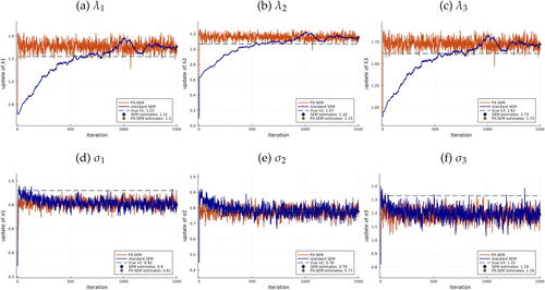
As shown in Figure 2, for all the parameters, PX-SEM converges almost immediately. However, for SEM, although it also converges relatively fast for $\sigma \prime s$, a notable difference is observed in the case of $\lambda \prime s$: it does not converge until 500 iterations.

Regarding volatilities of updates across iterations, Appendix D presents figures with longer trajectories, where we can observe that PX-SEM exhibits smaller volatilities. Appendix D also includes results for larger sample sizes and additional figures plotting cumulative computing time, revealing significant gains, especially for larger samples.

5 Discrete Choice Models

The second type of model we discuss is the random effects discrete choice model with persistent and transitory components. Discrete choice models are widely used in empirical research on various topics, including labor supply (Hyslop 1999) and consumer demand (Keane et al. 2013), among others. Distinguishing heterogeneity from persistence is of interest for many reasons, but the nonlinearity and the presence of latent variables complicate the estimation process.¹⁸

In this section, we develop PX-SEM algorithms for a group of discrete choice models with rich latent-variable structures, including time-invariant, persistent, and transitory components. Specifically, the O model is as follows: $$\begin{array}{c}{y}_{\mathit{\text{it}}}=\mathbb{1}(z_{\mathit{\text{it}}}>0),\\ z_{\mathit{\text{it}}}=\beta \prime x_{\mathit{\text{it}}}+{\mu }_i+{\nu }_{\mathit{\text{it}}}+{ϵ}_{\mathit{\text{it}}},\\ {\nu }_{\mathit{\text{it}}}=\rho {\nu }_{i,t-1}+u_{\mathit{\text{it}}},\end{array}$$where ${\mu }_i|x\stackrel{\text{iid}}{\sim }N(0,{\sigma }_{\mu }^2),{\nu }_{i1}|x\stackrel{\text{iid}}{\sim }N(0,1),u_{\mathit{\text{it}}}|x\stackrel{\text{iid}}{\sim }N(0,{\sigma }_u^2),{ϵ}_{\mathit{\text{it}}}|x\stackrel{\text{iid}}{\sim }N(0,1)$; and μ_i, u_it, ϵ_it are mutually independent.¹⁹

For each individual $i=1,\dots ,N$ at period $t=1,\dots ,T$, we observe a vector of independent variable x_it of dimension J and a binary (0-1) discrete dependent variable y_it, whereas z_it, individual effect μ_i, persistent component ν_it, and transitory component ϵ_it are latent. We denote the set of unknown parameters as θ, where $\theta \equiv (\beta ,{\sigma }_{\mu },\rho ,{\sigma }_u)$.

SEM

Let $z_i\equiv [z_{i1}\dots z_{\mathit{\text{iT}}}]\prime ,{\nu }_i\equiv [{\nu }_{i1}\dots {\nu }_{\mathit{\text{iT}}}]\prime$. From an initial guess ${\widehat{\theta }}^{(0)}$, we iterate through E-step and M-step for $s=0,1,\dots ,S$ until ${\widehat{\theta }}^{(s)}$ converges to the stationary distribution:

1. Stochastic E step: Draw $(z_i,{\mu }_i,{\nu }_i)$ from the posterior distribution $f_O(z_i,{\mu }_i,{\nu }_i|y_i,x_i;{\widehat{\theta }}^{(s)})$.

2. M step: Update ${\widehat{\theta }}^{(s+1)}=({\widehat{\beta }}^{(s+1)},{\widehat{\sigma }}_{\mu }^{(s+1)},{\widehat{\rho }}^{(s+1)},{\widehat{\sigma }}_u^{(s+1)})$

   $\begin{array}{c}{\widehat{\beta }}^{(s+1)}={(\sum _i\sum _t{x}_{\mathit{\text{it}}}{x}_{\mathit{\text{it}}}^{\prime })}^{-1}(\sum _i\sum _t{x}_{\mathit{\text{it}}}(z_{\mathit{\text{it}}}-{\mu }_i-{\nu }_{\mathit{\text{it}}})),\\ {\widehat{\rho }}^{(s+1)}={(\sum _i\sum _t{\nu }_{i,t-1}{\nu }_{i,t-1}^{\prime })}^{-1}(\sum _i\sum _t{\nu }_{i,t-1}{\nu }_{\mathit{\text{it}}}),\\ {\widehat{\sigma }}_{\mu }^{(s+1)}=\widehat{\text{std}}({\mu }_i)\text{ and }{\widehat{\sigma }}_u^{(s+1)}=\widehat{\text{std}}({\nu }_{\mathit{\text{it}}}-{\widehat{\rho }}^{(s+1)}{\nu }_{i,t-1}).\end{array}$

PX-SEM

One option for building the L model is to expand the O model to include only contemporaneous correlations, similar to the dynamic factor model in Section 4. Its advantage lies in the MLE being readily obtained in the PX-M step due to a separable likelihood. Appendix E provides the detailed steps and results of this approach. However, to achieve faster convergence, we now propose a more flexible L model.

Let us define $x_i\equiv {[x_{i1}^{\prime }\dots x_{\mathit{\text{iT}}}^{\prime }]}^{\prime },{ϵ}_i\equiv [{ϵ}_{i1}\dots {ϵ}_{\mathit{\text{iT}}}]\prime ,{\nu }_i^{*}\equiv [{\nu }_{i1}^{*}\dots {\nu }_{\mathit{\text{iT}}}^{*}]\prime ,{ϵ}_i^{*}\equiv [{ϵ}_{i1}^{*}\dots {ϵ}_{\mathit{\text{iT}}}^{*}]\prime$, and $z_i^{*}\equiv [z_{i1}^{*}\dots z_{\mathit{\text{iT}}}^{*}]\prime$. We construct the following L model: $$\begin{array}{c}{y}_{\mathit{\text{it}}}=\mathbb{1}(z_{\mathit{\text{it}}}>0),\mathrm{\hspace{1em}}\mathrm{\hspace{1em}}(L\mathit{\text{Model}})\\ z_{\mathit{\text{it}}}={\gamma }_t^{\prime }{x}_i+{\mu }_i+{\nu }_{\mathit{\text{it}}}+{ϵ}_{\mathit{\text{it}}},\\ {\left[{\mu }_i{\nu }_i^{\prime }{ϵ}_i^{\prime }\right]}^{\prime }=\mathit{\text{pA}}{\left[{\mu }_i^{*}{\nu }_i^{*\prime }{ϵ}_i^{*\prime }\right]}^{\prime }+B{x}_i,\\ {\nu }_{\mathit{\text{it}}}^{*}=\rho {\nu }_{i,t-1}^{*}+u_{\mathit{\text{it}}},\end{array}$$where ${\mu }_i^{*}|x\stackrel{\text{iid}}{\sim }N(0,{\sigma }_{\mu }^2),{\nu }_{i1}^{*}|x\stackrel{\text{iid}}{\sim }N(0,1),u_{\mathit{\text{it}}}|x\stackrel{\text{iid}}{\sim }N(0,{\sigma }_u^2),{ϵ}_{\mathit{\text{it}}}^{*}|x\stackrel{\text{iid}}{\sim }N(0,1)$, and ${\mu }_i^{*}$, u_it, ${ϵ}_{\mathit{\text{it}}}^{*}$ are mutually independent; and subject to $\frac{1}{p}\times (\mathit{\text{CB}}+\gamma )=I_{T\times T}\otimes \beta \prime ,\mathit{\text{CAΣA}}\prime C\prime =C\Sigma C\prime$, and $p>0$, where $C=[{\stackrel{\rightharpoonup }{1}}_{T\times 1}{I}_{T\times T}{I}_{T\times T}],\Sigma =\text{var}([{\mu }_i^{*}{\nu }_i^{*\prime }{ϵ}_i^{*\prime }]\prime ),\gamma \prime \equiv [{\gamma }_1\dots {\gamma }_T]$ and A is a lower triangular matrix with positive diagonal entries. Alongside θ from the O model, the L model contains a vector of auxiliary parameters $K\equiv [\text{vech}(A)\prime ,\text{vec}(B)\prime ,p]\prime$.

Following the linear expansion method, we introduce latent variables ${\mu }_i^{*},{\nu }_i^{*}$, and ${ϵ}_i^{*}$, which follow the same distributions as their O model counterparts. However, the E-step draws for $[{\mu }_i{\nu }_i^{\prime }ϵ{\prime }_i]$, given x_i, can result from an affine transformation applied to $[{\mu }_i^{*}{\nu }_i^{*\prime }{ϵ}_i^{*\prime }]$, allowing for linear correlations among μ_i, ν_i, ϵ_i, and dependence on x_i. The scalar p permits scaling z_it and thus the deviation of $\text{var}({ϵ}_{\mathit{\text{it}}})$ from the value of 1. Hence, the L model satisfies condition (a): when $B=0_{(2T+1)\times (J\times T)},A=I_{(2T+1)\times (2T+1)},p=1$, the two models coincide $f_O(y_i,z_i,{\mu }_i,{\nu }_i|x_i;\theta )=f_L(y_i,z_i,{\mu }_i,{\nu }_i|x_i;\theta ,A=I,B=\stackrel{\rightharpoonup }{0},p=1)$.

The L model has two key constraints: $\frac{1}{p}\times (\mathit{\text{CB}}+\gamma )=I_{T\times T}\otimes \beta \prime$ and $\mathit{\text{CAΣA}}\prime C\prime =C\Sigma C\prime$. Beyond addressing identification, these constraints simplify the reduction function. Specifically, under these constraints, the L model can be written as $z_i=p\beta \prime x_{\mathit{\text{it}}}+\mathit{\text{pC}}[{\mu }_i^{*}{\nu }_i^{*\prime }{ϵ}_i^{*\prime }]\prime$, implying no effect of auxiliary parameters p, A, and B on the conditional distribution of y_it given x_it. Therefore, regarding condition (b), we find a reduction function, $R(\theta ,K)=\theta$, satisfying $f_O(y_i|x_i;R(\theta ,K))=f_L(y_i|x_i;\theta ,K)$.

Finally, with the L model specified and an initial guess ${\widehat{\theta }}^{(0)}$, we iterate through the following two steps for $s=0,1,\dots ,S$ until ${\widehat{\theta }}^{(s)}$ converges to the stationary distribution:

1. Stochastic E step: Draw $(z_i,{\mu }_i,{\nu }_i)$ from the posterior distribution $f_O(z_i,{\mu }_i,{\nu }_i|y_i,x_i;{\widehat{\theta }}^{(s)})$.

2. PX-M step:

   1. L model estimation:

      ${\widehat{\theta }}_L,\widehat{K}=\text{arg} {\mathrm{\text{min}}}_{\theta ,K}\sum _i\Psi (\theta ,K;y_i,z_i,x_i,{\mu }_i,{\nu }_i)$

   2. Reduction: ${\widehat{\theta }}^{(s+1)}=R({\widehat{\theta }}_L,\widehat{K})={\widehat{\theta }}_L$

      where $\Psi (·)$ is a known function whose detailed specification is presented in Appendix F. Below, we list the moments involved in function $\Psi (·)$:

      $\begin{array}{c}p\beta :\hspace{1em}E(x_{\mathit{\text{it}}}(z_{\mathit{\text{it}}}-p\beta \prime x_{\mathit{\text{it}}}))=0,\frac{1}{p}\times (\mathit{\text{CB}}+\gamma )=I_{T\times T}\otimes \beta \prime \\ B:\hspace{1em}E(x_i([{\mu }_i{\nu }_i^{\prime }{ϵ}_i^{\prime }]-x{\prime }_{i}B\prime ))=0\\ {\sigma }_{\mu },p,\Sigma ,A:\mathit{\text{\hspace{1em}CAΣA}}\prime C\prime =C\Sigma C\prime ,\text{and moment constraints on }\Sigma \\ \rho ,{\sigma }_u:\hspace{1em}E({\nu }_{i,t-1}^{*}({\nu }_{\mathit{\text{it}}}^{*}-\rho {\nu }_{i,t-1}^{*}))=0,\text{var}({\nu }_{\mathit{\text{it}}}^{*}-\rho {\nu }_{i,t-1}^{*})={\sigma }_u^2.\end{array}$

Simulation Results

We conduct simulations to compare SEM and PX-SEM from a DGP with true parameter values: $\beta =[1.0;0.5],{\sigma }_{\mu }=1.25,\rho =0.7$, and ${\sigma }_u=0.9$.

The initial guess is determined as follows: (a) ${\widehat{\beta }}^{(0)}$ is the Probit regression coefficients of y_it on x_it, (b) Impose ${\widehat{\rho }}^{(0)}=1$, and the rest of the parameters are estimates of the linearly approximated model.²⁰ In the E-step, we employ a random-walk Metropolis-Hastings sampler with an acceptance rate controlled between 20% and 40%.

Figure 3 presents the estimation results of one simulation with N = 5000 and T = 8. Specifically, we plot the M-step updates ${\widehat{\theta }}^{(s)}$ for 1000 iterations (S = 1000). The blue line depicts each update of SEM, while the orange one represents the PX-SEM updates. In this example, we might be interested in switching to SEM, which is likelihood-based, treating the PX-SEM estimate as an initial guess. Hence, we also present the results of a combined approach, where we run PX-SEM for 500 iterations and then continue with SEM for another 500 iterations, using the average of the last 250 PX-SEM iterations as the initial guess, as shown by the gray line.²¹ The green dashed line indicates the true value. The final estimates are the average of the last 250 iterations ($S^0=250$), represented by the blue diamond for SEM, the orange star for PX-SEM, and the gray circle for PX-SEM + SEM.

Fig. 3 SEM and PX-SEM iterations of ${\widehat{\theta }}^{(s)}$ from an informed guess.

NOTE: Iterations of SEM (blue line), PX-SEM (orange line), and PX-SEM + SEM (gray line) based on 100 MH draws, compared with the true value (green dashed line). Estimates of SEM (blue diamond), PX-SEM (orange star), and PX-SEM + SEM (gray circle) are the average of the last 250 iterations. Informed initial guess.

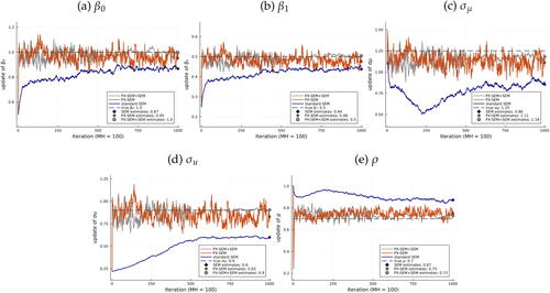
From this comparison, it is clear that starting from the same initial guess, PX-SEM converges almost immediately (within 100 iterations). In contrast, SEM progresses much slower, especially for ${\widehat{\sigma }}_{\mu }^{(s)},{\widehat{\sigma }}_u^{(s)}$, and ${\widehat{\rho }}^{(s)}$, and does not converge within 1000 iterations. In terms of the combined approach, the variation across iterations significantly decreases after transitioning to SEM. However, since the final estimates are the average of the last 250 updates, the difference between PX-SEM and PX-SEM + SEM is small.²²

Appendix L provides additional figures where the x-axis is the cumulative computing time. The gain is significant: SEM takes approximately 3000 sec to run 1000 iterations without converging, while PX-SEM converges almost immediately.²³

Appendix H compares algorithms based on random initial guesses. Researchers often run SEM algorithms from various initial guesses and choose one based on specific criteria (e.g., the likelihood value) to avoid obtaining a local maximum, given that getting a “good” initial guess can be challenging. Appendix H shows that the dominance of PX-SEM in convergence rate remains under random initial guesses. Given that this type of exercise is often performed repeatedly in practice, the time saved could be substantial.²⁴

Finally, Appendix M provides the overall trajectories of SEM and PX-SEM over iterations. Specifically, we conduct 40 simulations using the same DGP, each estimated under a different set of initial guesses shared by both SEM and PX-SEM. For each parameter, we examine the distribution of updates across 40 trajectories at each specific iteration and how this distribution evolves over the iterations for SEM and PX-SEM, respectively. We reach the same conclusion: PX-SEM significantly improves algorithmic efficiency.

6 Quantile Models

The final type of model for which we consider a PX-SEM approach is the persistent-transitory dynamic quantile models with individual effects, as proposed by Arellano, Blundell, and Bonhomme (2017) (referred to as ABB hereafter). The ABB model does not impose functional-form restrictions on the distributions of individual effects, transitory shocks, or conditional distributions of the persistent component. Indeed, the flexible dynamics of the persistent component allow for attractive features such as nonlinear persistence, meaning that the persistence could vary with the size of shocks and accumulated history, which is shown to be empirically prominent in earning dynamics. The model has also been applied to other topics including firm and health dynamics.

Specifically, we focus on the ABB baseline model with an additive fixed effect, discussed in their Appendix.²⁵ Denote the τth conditional quantile of ν_it given ${\nu }_{i,t-1}$ as $Q_{\nu }({\nu }_{i,t-1},\tau )$ for each $\tau \in (0,1)$. The O model to be estimated is as follows:

$\begin{array}{c}{y}_{\mathit{\text{it}}}={\mu }_i+{\nu }_{\mathit{\text{it}}}+{ϵ}_{\mathit{\text{it}}},\\ {\nu }_{\mathit{\text{it}}}=Q_{\nu }({\nu }_{i,t-1},u_{\mathit{\text{it}}}),\\ (u_{\mathit{\text{it}}}|{\mu }_i,u_{i,t-1},u_{i,t-2},\dots )\stackrel{\text{iid}}{\sim }\text{Uniform}(0,1),t=2,\dots ,T,\end{array}$ (O Model)where ϵ_it has zero mean, iid over time, and independent of ${\nu }_i\equiv [{\nu }_{i1}{\nu }_{i2}\dots {\nu }_{\mathit{\text{iT}}}]\prime$ and μ_i. Individual effect μ_i is assumed to be independent of ${ϵ}_i\equiv [{ϵ}_{i1}{ϵ}_{i2}\dots {ϵ}_{\mathit{\text{iT}}}]\prime$ and ν_i.

To estimate this model, we follow Arellano, Blundell, and Bonhomme (2017) and empirically specify the quantile function of ν_it given ${\nu }_{i,t-1},Q_{\nu }({\nu }_{i,t-1},\tau )$, the quantile function of ϵ_it, $Q_{ϵ}(\tau )$, the quantile function of ${\nu }_{i1},Q_{{\nu }_1}(\tau )$, and the quantile function of μ_i, $Q_{\mu }(\tau )$, as follows: $$\begin{array}{c}{Q}_{\nu }({\nu }_{i,t-1},\tau )=\sum _{h=0}^H{\gamma }_h^Q(\tau ){\phi }_h({\nu }_{i,t-1}),\\ Q_{ϵ}(\tau )={\gamma }^{ϵ}(\tau ),Q_{{\nu }_1}(\tau )={\gamma }^{{\nu }_1}(\tau ),Q_{\mu }(\tau )={\gamma }^{\mu }(\tau ),\end{array}$$where ${\phi }_h(·)$ is Hermite polynomials of order h and $\gamma (·)\prime s$ are functions to be estimated.

Arellano, Blundell, and Bonhomme (2017) exploit a variation of SEM for estimation, where the M-step involves a series of quantile regressions instead of likelihood optimization for computational convenience. We first explain their procedures. Let θ denote the set of unknown parameters, including ${\gamma }_k^Q(\tau ),{\gamma }^{ϵ}(\tau ),{\gamma }^{{\nu }_1}(\tau )$, and ${\gamma }^{\mu }(\tau )$.²⁶ With an initial guess ${\widehat{\theta }}^{(0)}$, we iterate through the following two steps until ${\widehat{\theta }}^{(s)}$ converges to the stationary distribution:

1. Stochastic E step: Draw μ_i and ν_i from the posterior distribution $f_O({\mu }_i,{\nu }_i|y_i;{\widehat{\theta }}^{(s)})$.

2. M step: Update parameters by computing a series of quantile regressions:

   $\begin{array}{c}{\widehat{\gamma }}^Q(\tau )=\text{arg} {\mathrm{\text{min}}}_{{\gamma }_0^Q,\dots ,{\gamma }_H^Q}{\sum }_{i=1}^N{\sum }_{t=2}^T{\rho }_{\tau }({\nu }_{\mathit{\text{it}}}-{\sum }_{h=0}^H{\gamma }_h^Q{\phi }_h({\nu }_{i,t-1})),\\ {\widehat{\gamma }}^{\mu }(\tau )=\text{arg} {\mathrm{\text{min}}}_{{\gamma }^{\mu }}{\sum }_{i=1}^N{\rho }_{\tau }({\mu }_i-{\gamma }^{\mu }),\\ {\widehat{\gamma }}^{ϵ}(\tau )=\text{arg} {\mathrm{\text{min}}}_{{\gamma }^{ϵ}}{\sum }_{i=1}^N{\sum }_{t=1}^T{\rho }_{\tau }({ϵ}_{\mathit{\text{it}}}-{\gamma }^{ϵ}),\\ {\widehat{\gamma }}^{{\nu }_1}(\tau )=\text{arg} {\mathrm{\text{min}}}_{{\gamma }^{{\nu }_1}}{\sum }_{i=1}^N{\rho }_{\tau }({\nu }_{i1}-{\gamma }^{{\nu }_1}),\end{array}$

   where ${\rho }_{\tau }(u)=u(\tau -\mathbb{1}(u\le 0))$ is the check function.

PX-SEM

We expand the O model linearly targeting the correlations among μ_i, ν_i, and ϵ_i. Define ${\nu }_i^{*}\equiv [{\nu }_{i1}^{*}\cdots {\nu }_{\mathit{\text{iT}}}^{*}]\prime ,{ϵ}_i^{*}\equiv [{ϵ}_{i1}^{*}\cdots {ϵ}_{\mathit{\text{iT}}}^{*}]\prime$. We build the following L model:

$\begin{array}{c}{y}_{\mathit{\text{it}}}={\mu }_i+{\nu }_{\mathit{\text{it}}}+{ϵ}_{\mathit{\text{it}}},\\ {[{\mu }_i{\nu }_i^{\prime }{ϵ}_i^{\prime }]}^{\prime }=A{[{\mu }_i^{*}{\nu }_i^{*\prime }{ϵ}_i^{*\prime }]}^{\prime },\\ {\nu }_{\mathit{\text{it}}}^{*}=Q_{\nu }({\nu }_{i,t-1}^{*},u_{\mathit{\text{it}}}),\\ (u_{\mathit{\text{it}}}|{\mu }_i^{*},u_{i,t-1},u_{i,t-2},\dots )\stackrel{\text{iid}}{\sim }\text{Uniform}(0,1),t=2,\dots ,T,\end{array}$ (L Model)subject to $\mathit{\text{CA}}=C$, where $C=[{\stackrel{\rightharpoonup }{1}}_{T\times 1}{I}_{T\times T}{I}_{T\times T}]$. Similarly, we assume that ${ϵ}_{\mathit{\text{it}}}^{*}$ has zero mean, iid over time, and independent of ${\nu }_i^{*}$ and ${\mu }_i^{*}$, and ${\mu }_i^{*}$ is independent of ${\nu }_i^{*}$. The L model contains a vector of auxiliary parameters $K\equiv \text{vec}(A)$.

Consistent with the linear expansion method, E-step draws $[{\mu }_i\nu {\prime }_iϵ{\prime }_i]\prime$ are assumed to be outcomes of affine transformations through matrix A of $[{\mu }_i^{*}{\nu }_i^{*\prime }{ϵ}_i^{*\prime }]\prime$, which follow identical distributions as their O model counterparts. When $A=I$, two models coincide, satisfying condition (a). Moreover, with the constraint $\mathit{\text{CA}}=C$, the L model becomes $y_i=C{[{\mu }_i^{*}{\nu }_i^{*\prime }{ϵ}_i^{*\prime }]}^{\prime }$, implying no effect of K on the observed-data likelihood. Thus, regarding condition (b), the reduction function is $R(\theta ,K)=\theta$.

Finally, with this L model and an initial guess ${\widehat{\theta }}^{(0)}$, we iterate through the following two steps for $s=0,1,,\dots ,S$ until ${\widehat{\theta }}^{(s)}$ converges to the stationary distribution:

1. Stochastic E step: Draw μ_i and ν_i from posterior distribution $f_O({\mu }_i,{\nu }_i|y_i;{\widehat{\theta }}^{(s)})$

2. PX-M step:

   1. L model estimation:

      ${\widehat{\theta }}_L,\widehat{K}=\text{arg} {\mathrm{\text{min}}}_{\theta ,K}\sum _i\Psi (\theta ,K;y_i,{\mu }_i,{\nu }_i)$

   2. Reduction: ${\widehat{\theta }}^{(s+1)}=R({\widehat{\theta }}_L,\widehat{K})={\widehat{\theta }}_L$

      where $\Psi (·)$ is a known function to be discussed in the following paragraphs.

The inclusion of matrix A adds complexity to joint estimation due to infeasible separate quantile regressions as in the SEM M-step and the involvement of many more parameters.²⁷ Thus, we employ two strategies: adding extra constraints on the entries of matrix A and sequential estimation.

Regarding the extra constraints, we assume that ϵ_it is orthogonal to ${\mu }_i^{*},{ϵ}_{i1}^{*}$,…, ${ϵ}_{i,t-1}^{*}$, for $t=2,\dots ,T$, and the coefficient of ${ϵ}_{\mathit{\text{it}}}^{*}$ with respect to ϵ_it is homogenous across all periods. The advantage of doing so is that, by exploiting moment conditions including zero correlation among ${\mu }_i^{*},{\nu }_i^{*}$, and ${ϵ}_i^{*}$, and ${\nu }_{\mathit{\text{it}}}^{*}$ following the first-order Markov process as well as ${ϵ}_{\mathit{\text{it}}}^{*}$ being iid, we can separately estimate matrix A through constrained GMM while restricting the number of unknowns to only two. This further facilitates the sequential estimation strategy. Once obtaining $\widehat{A}$, we estimate θ through the same series of quantile regressions as in SEM using ${[{\widehat{\mu }}_i^{*}{\widehat{\nu }}_i^{*\prime }{\widehat{ϵ}}_i^{*\prime }]}^{\prime }={\widehat{A}}^{-1}{[{\mu }_i{\nu }_i^{\prime }{ϵ}_i^{\prime }]}^{\prime }$. Appendix I provides a detailed discussion of the estimation process.²⁸

Simulation Results

We simulate from the following DGP ($N=5000,T=6$): (7) $$\begin{array}{c}{y}_{\mathit{\text{it}}}={\mu }_i+{\nu }_{\mathit{\text{it}}}+{ϵ}_{\mathit{\text{it}}},\\ {\nu }_{\mathit{\text{it}}}={\rho }_{\nu }{\nu }_{i,t-1}+({\sigma }_{\nu t0}+{\sigma }_{\nu t1}{\nu }_{i,t-1}^2)v_{\mathit{\text{it}}},\end{array}$$(7) where ${\mu }_i\stackrel{\text{iid}}{\sim }N(0,{\sigma }_{\mu }^2),{\nu }_{i1}\stackrel{\text{iid}}{\sim }N(0,{\sigma }_{\nu 1}^2),v_{\mathit{\text{it}}}\stackrel{\text{iid}}{\sim }N(0,1),{ϵ}_{\mathit{\text{it}}}\stackrel{\text{iid}}{\sim }N(0,{\sigma }_{ϵ}^2)$, and μ_i, ${\nu }_{i1}$, v_it, ϵ_it are mutually independent.

We present results for a persistent-transitory process without time-invariant heterogeneity and heteroscedasticity in the persistent shock by imposing ${\mu }_i=0$ and ${\sigma }_{\nu t1}=0$. The other parameter values are ${\rho }_{\nu }=0.8,{\sigma }_{\nu t0}=0.15,{\sigma }_{\nu t1}=0,{\sigma }_{\nu 1}^2=0.15,{\sigma }_{ϵ}^2=0.05$. Appendix J provides simulation results for a DGP with time-invariant heterogeneity and heteroscedasticity and another DGP, which is based on a flexible quantile model.

With the simulated data, we estimate the quantile model with time-invariant heterogeneity, as specified previously (the O model), assuming no knowledge of the distribution family. We set the initial guess by estimating the canonical random-walk permanent-transitory model, with details explained in Appendix J. Finally, the highest order of Hermite polynomials for the empirical specification of the ν_it dynamics, H, is set to two.

Figure 4 presents the results. To provide clearer visualization, instead of plotting the updates of raw parameters in the quantile model directly (due to their large quantity), we plot the iterations of estimated parameter values in the parametric model, (7). Specifically, in each iteration, we estimate the parametric model using E-step draws (μ, ν, and ϵ) for SEM and” corrected” draws (${\widehat{\mu }}^{*},{\widehat{\nu }}^{*}$, and ${\widehat{ϵ}}^{*}$) for PX-SEM. Importantly, these estimates are only for visualizing convergence and are not directly involved in the algorithm updating procedure. Consistent with previous exercises, PX-SEM exhibits rapid convergence for all parameters, whereas SEM converges much more slowly.

Fig. 4 SEM and PX-SEM iterations, ${\mu }_i=0$.

NOTE: Iterations of SEM (blue solid line) and PX-SEM (orange solid line) based on 100 MH draws, compared with the true value (green dashed line). In each iteration, we estimate the parametric model, (7), using E-step draws μ, ν, ϵ for SEM and “corrected” draws ${\widehat{\mu }}^{*},{\widehat{\nu }}^{*}$, ${\widehat{ϵ}}^{*}$ for PX-SEM. These estimates are only used for visualizing the convergence and are not directly involved in any algorithm. SEM estimates (blue diamond) and PX-SEM estimates (orange star) are both calculated as the average of the last 100 iterations. Informed initial guess.

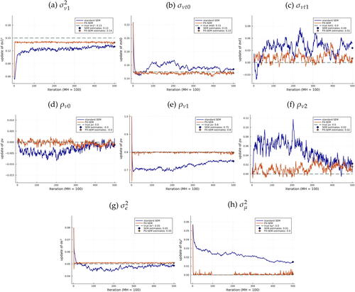
Appendix L provides complementary figures to Figure 4, with cumulative computing time as the x-axis, showing significant time gain: SEM takes over 5500 sec for 500 iterations without clear convergence, whereas PX-SEM converges almost immediately.²⁹ Appendix M presents the overall trajectories of 40 iterations. Finally, Appendix K shows simulation results for different sample sizes.

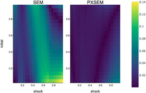
After 500 iterations, averaging the last 100 updates as temporary estimates, we simulate from the estimated models and compare the model fit, focusing on the persistence of the ν_it dynamics, $\frac{\partial {\nu }_{\mathit{\text{it}}}}{\partial {\nu }_{i,t-1}}({\nu }_{i,t-1},\tau )$, one of the characteristics of interest (Arellano, Blundell, and Bonhomme 2017). Figure 5 displays heatmaps showing the absolute distance between the estimated persistence and true persistence at different levels of the shock τ and ${\nu }_{i,t-1}$ for SEM and PX-SEM, respectively. Overall, PX-SEM shows a better model fit.

Fig. 5 Distance between estimated persistence and true persistence, ${\mu }_i=0$. NOTE: The absolute distance between the estimated ν_t persistence (based on the average of the last 100 iterations) and true persistence for each level of the shock τ and ${\nu }_{i,t-1}$.

7 Conclusions

This article introduces new estimation algorithms for dynamic panel data models with latent variables. By combining the parameter expansion ideas with the SEM algorithm, we develop the PX-SEM algorithm, which could facilitate convergence in models with a large space of latent variables by improving algorithmic efficiency.

Sharing the same E-step as SEM, PX-SEM differs in the M-step. Instead of estimating the original model (the O model), the M-step of PX-SEM requires estimating an expanded model (the L model). Effectively, we propose new estimators for the pseudo-data within iterations, accounting for the misspecification of the O model for draws based on parameter values far from the truth. Thus, PX-SEM can leverage additional model information to effectively” correct” the M-step updates in progressing to more accurate ones.

Moreover, the article proposes a method for constructing the L model through linear expansion and presents new PX-SEM-based estimation algorithms for three types of dynamic panel data models: factor models, discrete choice models, and quantile models.

Regarding statistical properties, we establish the asymptotic equivalence of the likelihood-based PX-SEM to an alternative SEM with a smaller expected fraction of missing information compared to the standard O model based SEM, implying a faster global convergence rate and a smaller variance for the limiting stationary distribution. Finally, simulations show that PX-SEM can significantly improve the algorithmic efficiency relative to SEM.

Supplementary Materials

The online supplement consists of the following appendices. Appendix A presents illustrative figures for the intuition behind PX-SEM and comparisons among different L models and M-step estimators using the toy model. Appendix B provides a detailed proof for Section 3. Appendix C explains the equivalence through reparameterization among L models. Appendices E, F, and G discuss alternative L models, detailed L model estimation procedures, and PX-SEM methods applied to two extensions for the discrete choice model in Section 5. Appendix I provides detailed L model estimation procedures for the quantile model in Section 6. Appendices D, H, J–M present more simulation results for the three types of models discussed in Sections 4-6, with more iterations, different sample sizes, cumulative computing time, different initial guesses, and overall trajectories.

Acknowledgments

This work is based on Chapter 2 of my PhD thesis at CEMFI, which received the Enrique Fuentes Quintana Funcas Award in Economics, Finance and Business 2021-2022. I am deeply grateful to Manuel Arellano for his invaluable support and advice. I also thank Martin Almuzara, Dante Amengual, Dmitry Arkhangelsky, Orazio Attanasio, Richard Blundell, Stéphane Bonhomme, Micole De Vera, Jose Gutierrez, Pedro Mira, Josep Pijoan-Mas, Enrique Sentana, Liyang Sun, and seminar participants at IE university, CEMFI, International Panel Data Conference, EEA-ESEM, and SAEe meetings for valuable comments and suggestions. Two anonymous referees and an Associate Editor have helped greatly improve the article. All errors are my sole responsibility.

Disclosure Statement

The author reports there are no competing interests to declare.

Additional information

Funding

Grants PID2022-143184NA-I00 funded by MCIU/AEI/10.13039/501100011033 and by FEDER, UE; BES-2017-082506 funded by MCIU/AEI/10.13039/501100011033 and by “ESF Investing in your future”; and MDM-2016-0684 funded by MCIU/AEI/10.13039/501100011033 are greatly acknowledged.

Notes

1 Arellano and Bonhomme (2017) discusses the potentials of SEM in nonlinear panel data analysis.

2 For instance, Arellano et al. (2023) develops a Sequential Monte Carlo sampler for the E step.

3 Wei (2022) applies the algorithms developed in this article to a substantive analysis of the earnings and employment dynamics of older workers, which brings together elements of the three types of panel models considered here.

4 Liu, Rubin, and Wu (1998) is based on the EM algorithm; Liu and Wu (1999) applies the parameter expansion technique to Bayesian inference; Lavielle and Meza (2007) combines the parameter expansion technique with Monte Carlo EM (Wei and Tanner 1990).

5 See Wu (1983) for more discussions.

6 Since k does not affect the L model observed data likelihood, $f_O(y_i;{\sigma }_L)=f_L(y_i;{\sigma }_L,1)=f_L(y_i;{\sigma }_L,k_L)$

7 Note that the reduction function satisfies $R(\theta ,K_0)=\theta$.

8 In the moment-based PX-EM case, if the fixed point with K = K₀ exists, then it will satisfy $\sum _i(\int {\Psi }_O(Y_i^{*},W_i;\widehat{\theta })f_O(Y_i^{*}|W_i;\widehat{\theta })d{Y}_i^{*})=0$.

9 Note that the E-step draws of PX-SEM are based on the O model under the guess ${\widehat{\theta }}^{(s)}$. This is equivalent to making draws from the L model under the guess ${\widehat{\Theta }}^{(s)}=[{\widehat{\theta }}^{(s)};K_0]$, due to condition (a).

10 Appendix B shows that for any L model, an alternative L model can be found by reparameterization, which yields identical updates of θ with the reduction function $R(\theta ,K)=\theta$.

11 That A–V being positive definite implies $H_{\theta \theta }^{-1}-V_{\theta \theta }$ being positive definite.

12 The author thanks an anonymous referee for his/her encouragement to develop this result.

13 With a fixed S⁰, the PX-SEM and SEM estimators will in general give rise to different asymptotic variances. Expressions for these variances are provided in Appendix B.

14 In this expression, $Y_i^{*}$ also includes error terms in the measure equation $G(·)$.

15 Extensions include unit-specific matrix A (Section 4) and adding exogenous regressor X_i (Section 5).

16 The constraint might not be necessary in applications where reduction functions are easy to find.

17 The method can be easily adapted to models with (a) unknown persistence in the ν_t process, (b) multiple latent factors, (c) ϵ_it following an MA process, etc.

18 Chen (2016) proposes a fixed effects EM estimator for a class of nonlinear panel data models.

19 Appendix G presents two extensions: (a) Allowing for the dependence of μ_i and ${\nu }_{i1}$ on $x_{i1}$, and (b) Logit (with strategies for the quantile model in the next section).

20 We approximate the model as follows $y_{\mathit{\text{it}}}=\Phi (\beta \prime x_{\mathit{\text{it}}}+{\mu }_i+{\nu }_{\mathit{\text{it}}})+{\eta }_{\mathit{\text{it}}}\approx 0.5+0.25(\beta \prime x_{\mathit{\text{it}}}+{\mu }_i+{\nu }_{\mathit{\text{it}}})+{\eta }_{\mathit{\text{it}}}$.

21 We could also endogenize the switching procedure by using metrics like the distance between $\widehat{K}$ and K₀ or the likelihood difference between the L model and the O model to guide our transition to SEM.

22 Whether PX-SEM requires more iterations in this example due to its higher volatility, impacting total computing time, is beyond this article’s scope, especially considering the PX-SEM + SEM option.

23 The results are obtained using a Mac Mini (M1, 2020) with a single processor core. We apply the Metropolis-Hastings algorithm for the E-step, with the first 100 iterations designated as a burn-in phase.

24 Appendix H also presents simulation results with more iterations and different sample sizes.

25 In practice, standard SEM generally performs well in estimating the ABB baseline model without the fixed effect. But it is challenging when a fixed effect is included. We also remove age effects.

26 Unknown parameters also include tail parameters. Functions $\gamma (·)$ are piecewise-polynomial interpolating splines on a grid $[{\tau }_1,{\tau }_2],[{\tau }_2,{\tau }_3]$,…, $[{\tau }_{L-1},{\tau }_L]$. And the tails on $(0,{\tau }_1]$ and $[{\tau }_L,1)$ are modeled using a parametric model. Please refer to Appendix B in Arellano, Blundell, and Bonhomme (2017) for more details.

27 In the discrete choice model, the matrix A and other auxiliary parameters can be easily estimated in the PX-M step by focusing solely on the first two moments due to the normality assumption.

28 Similar strategies are used to estimate a Logit model in Appendix G.

29 The results are obtained using a Mac Mini (M1, 2020) with a single processor core. We apply the Metropolis-Hastings algorithm for the E-step, with the first 100 iterations designated as a burn-in phase.

References

- Arcidiacono, P., and Jones, J. B. (2003), “Finite Mixture Distributions, Sequential Likelihood and the EM Algorithm,” Econometrica, 71, 933–946. DOI: 10.1111/1468-0262.00431.
- Arellano, M., Blundell, R., and Bonhomme, S. (2017), “Earnings and Consumption Dynamics: A Nonlinear Panel Data Framework,” Econometrica, 85, 693–734. DOI: 10.3982/ECTA13795.
- Arellano, M., Blundell, R., Bonhomme, S., and Light, J. (2023), “Heterogeneity of Consumption Responses to Income Shocks in the Presence of Nonlinear Persistence,” Journal of Econometrics, 240, 105449. DOI: 10.1016/j.jeconom.2023.04.001.
- Arellano, M., and Bonhomme, S. (2016), “Nonlinear Panel Data Estimation via Quantile Regressions,” The Econometrics Journal, 19, C61–C94. DOI: 10.1111/ectj.12062.
- ———(2017), “Nonlinear Panel Data Methods for Dynamic Heterogeneous Agent Models,” Annual Review of Economics, 9, 471–496.
- Bai, J., and Ng, S. (2008), Large Dimensional Factor Analysis. Foundations and Trends[textregistered] in Econometrics (Vol. 3), pp. 89–163, Hanover, MA: Now Publishers. DOI: 10.1561/0800000002.
- Chen, M. (2016), “Estimation of Nonlinear Panel Models with Multiple Unobserved Effects,” Working Paper, Department of Economics, University of Warwick.
- Dempster, A. P., Laird, N. M., and Rubin, D. B. (1977), “Maximum Likelihood from Incomplete Data via the EM Algorithm,” Journal of the Royal Statistical Society, Series B, 39, 1–22. DOI: 10.1111/j.2517-6161.1977.tb01600.x.
- Diebolt, J., and Celeux, G. (1993), “Asymptotic Properties of a Stochastic EM Algorithm for Estimating Mixing Proportions,” Stochastic Models, 9, 599–613. DOI: 10.1080/15326349308807283.
- Geweke, J. (1977), “The Dynamic Factor Analysis of Economic Time Series,” in Latent Variables in Socio-Economic Models, eds. D. J. Aigner and A. S. Goldberger, Amsterdam: North-Holland.
- Hyslop, D. R. (1999), “State Dependence, Serial Correlation and Heterogeneity in Intertemporal Labor Force Participation of Married Women,” Econometrica, 67, 1255–1294. DOI: 10.1111/1468-0262.00080.
- Keane, M. P. (2013), “Panel Data Discrete Choice Models of Consumer Demand,” in The Oxford Handbook of Panel Data, ed. B. H. Baltagi, pp. 548–582, Oxford: Oxford University Press.
- Lavielle, M., and Meza, C. (2007), “A Parameter Expansion Version of the SAEM Algorithm,” Statistics and Computing, 17, 121–130. DOI: 10.1007/s11222-006-9007-6.
- Liu, C., Rubin, D. B., and Wu, Y. N. (1998), “Parameter Expansion to Accelerate EM: The px-em Algorithm,” Biometrika, 85, 755–770. DOI: 10.1093/biomet/85.4.755.
- Liu, J. S., and Wu, Y. N. (1999), “Parameter Expansion for Data Augmentation,” Journal of the American Statistical Association, 94, 1264–1274. DOI: 10.1080/01621459.1999.10473879.
- Nielsen, S. F. (2000), “The Stochastic EM Algorithm: Estimation and Asymptotic Results,” Bernoulli, 6, 457–489. DOI: 10.2307/3318671.
- Pastorello, S., Patilea, V., and Renault, E. (2003), “Iterative and Recursive Estimation in Structural Nonadaptive Models,” Journal of Business & Economic Statistics, 21, 449–509. DOI: 10.1198/073500103288619124.
- Stock, J. H., and Watson, M. W. (2006), “Forecasting with Many Predictors,” Handbook of Economic Forecasting, 1, 515–554.
- ———(2011), “Dynamic Factor Models,” in Oxford Handbook of Economic Forecasting, eds. Michael P. Clements and David F. Hendry, Oxford: Oxford University Press.
- Wei, G. C., and Tanner, M. A. (1990), “A Monte Carlo Implementation of the EM Algorithm and the Poor Man’s Data Augmentation Algorithms,” Journal of the American statistical Association, 85, 699–704. DOI: 10.1080/01621459.1990.10474930.
- Wei, S. (2022), “Income, Employment and Health Risks of Older Workers,” Documentos de Trabajo (CEMFI), (5), 1.
- Wu, C. J. (1983), “On the Convergence Properties of the EM Algorithm,” The Annals of Statistics, 11, 95–103. DOI: 10.1214/aos/1176346060.