Incorporating different sources of information for Bayesian optimal portfolio selection

Abstract

This paper introduces Bayesian inference procedures for tangency portfolios, with a primary focus on deriving a new conjugate prior for portfolio weights. This approach not only enables direct inference about the weights but also seamlessly integrates additional information into the prior specification. Specifically, it automatically incorporates high-frequency returns and a market condition metric (MCM), exemplified by the CBOE Volatility Index (VIX) and Economic Policy Uncertainty Index (EPU), significantly enhancing the decision-making process for optimal portfolio construction. While the Jeffreys prior is also acknowledged, emphasis is placed on the advantages and practical applications of the conjugate prior. An extensive empirical study reveals that our method, leveraging this conjugate prior, consistently outperforms existing trading strategies in the majority of examined cases.

Keywords:

• Conjugate prior
• EPU
• high-frequency data
• Jeffreys prior
• value-weighted portfolio
• VIX

Disclaimer

As a service to authors and researchers we are providing this version of an accepted manuscript (AM). Copyediting, typesetting, and review of the resulting proofs will be undertaken on this manuscript before final publication of the Version of Record (VoR). During production and pre-press, errors may be discovered which could affect the content, and all legal disclaimers that apply to the journal relate to these versions also.

1 Introduction

Since the seminal paper of Markowitz (1952), optimal portfolio theory has played a pivotal role in both theoretical finance research and practical applications. Its primary objective is to provide investors with a decision rule for optimal fund allocation. While various methods have been proposed in the literature over the past several decades (Markowitz, 1959; Ingersoll, 1987), recent advancements in computer technology, including faster processors and GPU computations, along with the availability of extensive datasets, have led to the development of novel approaches now discussed in both financial and statistical literature (Cai et al., 2020; Bauder et al., 2021; Ding et al., 2021; Kan et al., 2022; Lassance et al., 2022; Bodnar et al., 2023; Ding et al., 2023; Reh et al., 2023).

In scenarios where a risk-free asset is present in the financial market, optimal portfolio weights are typically obtained by solving the mean-variance optimization problem (sometimes referred to as maximum quadratic utility problem) (Ingersoll, 1987; Britten-Jones, 1999; Lassance et al., 2024)(1) $$\underset{\mathit{w}}{\max }\left\{{\mathit{w}}^{\mathrm{\top }}\mathit{\mu }-\frac{\gamma }{2}{\mathit{w}}^{\mathrm{\top }}\mathbf{\Sigma }\mathit{w}\right\},$$(1) where $\mathit{\mu }$ denotes the vector of the excess expected returns of the risky assets, $\mathbf{\Sigma }$ is its covariance matrix, and γ represents the coefficient of the investor’s risk aversion which is usually assumed to be known. By varying the risk aversion coefficient γ from 0 to $+\infty$, we obtain the weights for all optimal portfolios when a risk-free asset is present. The solution of the optimization problem (1) is known as the weights of the tangency portfolio which are given by(2) $${\mathit{w}}_{TP}={\gamma }^{-1}{\mathbf{\Sigma }}^{-1}\mathit{\mu }.$$(2)

The weights (2) determine the part of the investor wealth invested in the risky assets, while $1-{\mathit{1}}^{\mathrm{\top }}{\mathit{w}}_{TP}$ is invested in the risk-free asset.

A prevalent challenge in applying the mean-variance optimal portfolio, denoted as ${\mathit{w}}_{TP}$, is estimating the unknown mean vector $\mathit{\mu }$ and covariance matrix $\mathbf{\Sigma }$ using historical asset return data before portfolio construction. This issue, known as parameter uncertainty, has been thoroughly investigated in recent financial and statistical literature.

The classical approach to this problem involves replacing the unknown parameters $\mathit{\mu }$ and $\mathbf{\Sigma }$ with their sample estimators, leading to the creation of what is known in the literature as the sample tangency portfolio. The distributional properties and test theory based on the characteristics of the tangency portfolio have been studied and developed by various researchers (Jobson and Korkie, 1980, 1981; Okhrin and Schmid, 2006), with recent contributions addressing the distributional properties of large-dimensional tangency portfolios and establishing shrinkage-type estimators for tangency portfolio weights (Kan and Zhou, 2007; Bodnar et al., 2022a; Lassance et al., 2024).

Bayesian statistics offers an alternative for estimating tangency portfolio weights. In the Bayesian framework, unknown model parameters are treated as random variables, with prior beliefs and observed data jointly contributing to statistical inferences. This methodology has been utilized in portfolio theory since the 1960s, and numerous priors for $\mathit{\mu }$ and $\mathbf{\Sigma }$ have been proposed (Zellner and Chetty, 1965; Winkler, 1973; Bawa et al., 1979; Frost and Savarino, 1986; Rachev et al., 2008; Tu and Zhou, 2010; Avramov and Zhou, 2010; Bodnar et al., 2022b).

Early papers on Bayesian portfolio theory typically employed diffuse priors for $\mathit{\mu }$ and $\mathbf{\Sigma }$, while more recent studies have advocated for the use of informative priors. For instance, Stambaugh (1997) highlighted the preference for informative priors when certain risky assets have a longer historical record than others. Hierarchical priors were introduced by Jorion (1986) and Greyserman et al. (2006), and objective-based priors were examined in Tu and Zhou (2010). Furthermore, Bodnar et al. (2017) and Bauder et al. (2018) considered Bayesian inference procedures derived specifically for optimal portfolio weights. A Bayesian decision-theoretic approach presents another line of applications of Bayesian methods to portfolio theory (Hahn and Carvalho, 2015; Puelz et al., 2017, 2020). In this approach, the weights of optimal portfolios are no longer treated as functions of model parameters. Instead, they are considered as a decision rule in the decision-theoretic sense. Consequently, the optimization problem is constructed by involving the posterior predictive distribution (Puelz et al., 2020; Bauder et al., 2021).

A notable advantage of Bayesian over frequentist statistics is the ability to incorporate prior information into statistical analysis. Black and Litterman (1992) integrated economic beliefs into prior construction, while Pástor and Stambaugh (2000) and Pástor (2000) utilized asset pricing models to inform their priors. However, the specification of informative priors for the mean vector and covariance matrix of stock returns can be a complex task. Additionally, it is worth noting that these parameters are predominantly used for calculating optimal portfolio weights – the primary concern for portfolio managers.

In this paper, we contribute to the extant literature on Bayesian portfolio selection by developing a novel Bayesian approach that directly models optimal portfolio weights. This approach facilitates the assessment of weight uncertainty based on observed data and prior beliefs. Additionally, we introduce a unique method for specifying prior distributions in this new setup, using a combination of high-frequency data alongside a market condition metric (MCM), such as the CBOE Volatility Index (VIX) or Economic Policy Uncertainty Index (EPU). Through an empirical study, we compare our method with various existing approaches.

The remainder of the paper is structured as follows: Section 2 introduces an informative conjugate prior directly to tangency portfolio weights. Section 3 delves into hyperparameter selection, followed by Section 4, which showcases the empirical illustration results. Section 5 offers concluding remarks. Additionally, the supplementary material provides a detailed discussion on the application of a noninformative Jeffreys prior, contains the proofs supporting our theoretical results, and presents a stochastic representation for the tangency portfolio weights derived under a hierarchical prior.

2 Bayesian estimation of tangency portfolio weights

Let(3) $${\mathit{x}}_{1:n}=({\mathit{x}}_1,\dots ,{\mathit{x}}_n)=({\tilde{\mathit{x}}}_1-r_{f,1}\mathit{1},\dots ,{\tilde{\mathit{x}}}_n-r_{f,n}\mathit{1})$$(3) denote the data matrix comprised of n realizations of the p-dimensional vectors of excess (logarithmic) stock returns. Here, ${\tilde{\mathit{x}}}_i$ denotes the vector of stock returns, $r_{f,i}$ represents the return of the risk-free asset, and $\mathit{1}$ is a p-dimensional vector of ones. We assume that the excess stock returns are independent and normally distributed conditionally on their mean vector $\mathit{\mu }$ and covariance matrix $\mathbf{\Sigma }$. Note that although the conditional distribution of the excess stock returns is assumed to be normal and they are assumed to be conditionally independently distributed, their unconditional distribution is heavy-tailed and the stock returns are no longer unconditionally independent (Bernardo and Smith, 2000).

Under the above assumptions, the likelihood function of the stock returns is given by(4) $$\begin{array}{c}f({\mathit{x}}_{1:n}|\mathit{\mu },\mathbf{\Sigma })\propto \text{det}{(\mathbf{\Sigma })}^{-n/2}\hspace{0.17em}\exp \hspace{0.17em}\left(-\frac{1}{2}\sum _{i=1}^n{({\mathit{x}}_i-\mathit{\mu })}^{\mathrm{\top }}{\mathbf{\Sigma }}^{-1}({\mathit{x}}_i-\mathit{\mu })\right)\\ =\text{det}{(\mathbf{\Sigma })}^{-n/2}\hspace{0.17em}\exp \hspace{0.17em}\left(-\frac{n}{2}{\mathit{\mu }}^{\mathrm{\top }}{\mathbf{\Sigma }}^{-1}\mathit{\mu }\right)\end{array}$$(4) (5) $$\times \hspace{0.17em}\exp \hspace{0.17em}\left({\left(\sum _{i=1}^n{\mathit{x}}_i\right)}^{\mathrm{\top }}{\mathbf{\Sigma }}^{-1}\mathit{\mu }+\text{tr}\left({\mathbf{\Sigma }}^{-1}\left(-\frac{1}{2}\sum _{i=1}^n{\mathit{x}}_i{\mathit{x}}_i^{\mathrm{\top }}\right)\right)\right),$$(5) which is the density function of an exponential family (Sundberg, 2019) with canonical parameters(6) $$\mathit{\nu }={\mathbf{\Sigma }}^{-1}\mathit{\mu }\hspace{1em}\text{and}\hspace{1em}\Omega ={\mathbf{\Sigma }}^{-1},$$(6)

and canonical statistics $(\mathit{t},-\mathit{T}/2)$ with(7) $$\mathit{t}=\sum _{i=1}^n{\mathit{x}}_i\hspace{1em}\text{and}\hspace{1em}\mathit{T}=\sum _{i=1}^n{\mathit{x}}_i{\mathit{x}}_i^{\mathrm{\top }}.$$(7)

Note that $\mathit{\nu }$ is proportional to the weights of an optimal portfolio in the case when the risk-free rate is available, that is (Ingersoll, 1987; Britten-Jones, 1999)(8) $$\mathit{w}={\gamma }^{-1}{\mathbf{\Sigma }}^{-1}(\tilde{\mathit{\mu }}-r_f\mathit{1})={\gamma }^{-1}{\mathbf{\Sigma }}^{-1}\mathit{\mu }.$$(8)

As such, $\mathit{\nu }$ is the main parameter in the model (4), while $\Omega$ will be treated as a nuisance parameter matrix.

2.1 Conjugate prior

In this section, we derive a conjugate prior for parameters $\mathit{\nu }$ and $\Omega$, delegating the derivation of the Jeffreys prior to the supplementary material. A pivotal advantage of using a conjugate prior parameterized by $\mathit{\nu }$ and $\Omega$ instead of $\mathit{\mu }$ and $\mathbf{\Sigma }$ is its ability to seamlessly incorporate prior information about portfolio weights. This offers a potential advantage over the Black-Litterman model, which often requires complex formulations of views on asset returns (Black and Litterman, 1992). Furthermore, the conjugate prior allows for effortless integration of diverse types of information available in the capital market for the construction of optimal portfolios. Further elucidation on the incorporation of varied information sources is provided in Section 3. Thanks to its mathematical properties, the new conjugate prior also simplifies Bayesian analysis and inference about the portfolio weights.

Using the expression of the likelihood function (4), which belongs to the exponential family, the conjugate prior for $\mathit{\nu }$ and $\Omega$ is deduced as(9) $$\pi (\mathit{\nu },\Omega )\propto \text{det}{(\Omega )}^{n_0/2}\hspace{0.17em}\exp \hspace{0.17em}\left(-\frac{n_0}{2}{\mathit{\nu }}^{\mathrm{\top }}{\Omega }^{-1}\mathit{\nu }\right)\hspace{0.17em}\exp \hspace{0.17em}\left(c_0{\mathit{w}}_0^{\mathrm{\top }}{\mathit{S}}_0\mathit{\nu }+\text{tr}\left(\Omega \left(-\frac{1}{2}{\mathit{S}}_0\right)\right)\right),$$(9)

for hyperparameters c₀, n₀, ${\mathit{w}}_0$, and ${\mathit{S}}_0$. Rewriting (9) we get(10) $$\begin{array}{c}\pi (\mathit{\nu },\Omega )\propto \text{det}{(\Omega )}^{n_0/2}\hspace{0.17em}\exp \hspace{0.17em}\left(-\frac{1}{2}\text{tr}\left(\Omega \left({\mathit{S}}_0-c_0^2{n}_0^{-1}{\mathit{S}}_0{\mathit{w}}_0{\mathit{w}}_0^{\mathrm{\top }}{\mathit{S}}_0\right)\right)\right)\\ \times \hspace{0.17em}\exp \hspace{0.17em}\left(-\frac{n_0}{2}{(\mathit{\nu }-c_0{n}_0^{-1}\Omega {\mathit{S}}_0{\mathit{w}}_0)}^{\mathrm{\top }}{\Omega }^{-1}(\mathit{\nu }-c_0{n}_0^{-1}\Omega {\mathit{S}}_0{\mathit{w}}_0)\right).\end{array}$$(10)

Consequently, the prior information about $\mathit{\nu }$ and $\Omega$ is summarized as a conditional normal prior for $\mathit{\nu }$ and a Wishart prior for $\Omega$ expressed as(11) $$\mathit{\nu }|\Omega \sim {\mathcal{N}}_p\left(c_0{n}_0^{-1}\Omega {\mathit{S}}_0{\mathit{w}}_0,n_0^{-1}\Omega \right),$$(11) (12) $$\Omega \sim {\mathcal{W}}_p\left(n_0+p+2,{\mathit{S}}_0^{-1}+\frac{{\mathit{w}}_0{\mathit{w}}_0^{\mathrm{\top }}}{c_0^{-2}{n}_0-{\mathit{w}}_0^{\mathrm{\top }}{\mathit{S}}_0{\mathit{w}}_0}\right).$$(12)

Setting(13) $$c_0=\frac{-(n_0+p+2)+\sqrt{{(n_0+p+2)}^2+4n_0{\mathit{w}}_0^{\mathrm{\top }}{\mathit{S}}_0{\mathit{w}}_0}}{2{\mathit{w}}_0^{\mathrm{\top }}{\mathit{S}}_0{\mathit{w}}_0}$$(13) means that the unconditional prior mean of $\mathit{\nu }$ is ${\mathit{w}}_0$ and, hence, ${\mathit{w}}_0$ will reflect the prior belief about the portfolio weights.

Comparing the expression of the likelihood function (4) with the prior (9), one can conclude the matrix ${\mathit{S}}_0$ represents prior belief about the future value of the component of the canonical statistic given by ${\sum }_{i=1}^n{\mathit{x}}_i{\mathit{x}}_i^{\mathrm{\top }}$. Furthermore, from the equality(14) $${\left({\mathit{S}}_0^{-1}+\frac{{\mathit{w}}_0{\mathit{w}}_0^{\mathrm{\top }}}{c_0^{-2}{n}_0-{\mathit{w}}_0^{\mathrm{\top }}{\mathit{S}}_0{\mathit{w}}_0}\right)}^{-1}={\mathit{S}}_0-\frac{c_0^2}{n_0}{\mathit{S}}_0{\mathit{w}}_0{\mathit{w}}_0^{\mathrm{\top }}{\mathit{S}}_0$$(14) and the fact that (Gupta and Nagar, 2000, Section 3.4)(15) $${\Omega }^{-1}\sim {\mathcal{W}}_p^{-1}\left(n_0+2p+3,{\mathit{S}}_0-\frac{c_0^2}{n_0}{\mathit{S}}_0{\mathit{w}}_0{\mathit{w}}_0^{\mathrm{\top }}{\mathit{S}}_0\right),$$(15) we get that the prior mean of ${\Omega }^{-1}=\mathbf{\Sigma }$ is given by (Gupta and Nagar, 2000, Theorem 3.4.3)(16) $$\mathbb{E}\left({\Omega }^{-1}\right)=\frac{1}{n_0+1}\left({\mathit{S}}_0-\frac{c_0^2}{n_0}{\mathit{S}}_0{\mathit{w}}_0{\mathit{w}}_0^{\mathrm{\top }}{\mathit{S}}_0\right).$$(16)

Finally, we note that(17) $$c_0=\frac{2n_0}{(n_0+p+2)+\sqrt{{(n_0+p+2)}^2+4n_0{\mathit{w}}_0^{\mathrm{\top }}{\mathit{S}}_0{\mathit{w}}_0}}$$(17) (18) $$=\frac{2}{1+(p+2)/n_0+\sqrt{{(1+(p+2)/n_0)}^2+4{\mathit{w}}_0^{\mathrm{\top }}{\mathit{S}}_0{\mathit{w}}_0/n_0}}.$$(18)

As such, as n₀ is considerably larger than p and ${\mathit{w}}_0^{\mathrm{\top }}{\mathit{S}}_0{\mathit{w}}_0$, then c₀ tends to 1 and, hence, the prior mean of ${\Omega }^{-1}$ is approximated by a centralized version of ${\mathit{S}}_0$. Combining this observation with the fact that ${\mathit{S}}_0$ represents a prior belief about the value of ${\sum }_{i=1}^n{\mathit{x}}_i{\mathit{x}}_i^{\mathrm{\top }}$ and the formula for $\mathit{\nu }$ as in (6), it is concluded that the prior mean of ${\Omega }^{-1}$ is similar to the expression used in the definition of the sample covariance matrix in the frequentist statistics.

Next, we derive the posterior for $\mathit{\nu }$ and $\Omega$ when the conjugate prior (9) is employed. Let(19) $$n_c=n+n_0,\hspace{1em}{\mathit{S}}_c={\mathit{S}}_0+\mathit{T},\hspace{1em}\text{and}\hspace{1em}{\mathit{w}}_c={\mathit{S}}_c^{-1}(c_0{\mathit{S}}_0{\mathit{w}}_0+\mathit{t}).$$(19)

Then, it holds that(20) $$\begin{array}{c}\pi (\mathit{\nu },\Omega |{\mathit{x}}_{1:n})\propto \text{det}{(\Omega )}^{(n_0+n)/2}\hspace{0.17em}\exp \hspace{0.17em}\left(-\frac{n_0+n}{2}{\mathit{\nu }}^{\mathrm{\top }}{\Omega }^{-1}\mathit{\nu }\right)\\ \times \hspace{0.17em}\exp \hspace{0.17em}\left({(c_0{\mathit{S}}_0{\mathit{w}}_0+\mathit{t})}^{\mathrm{\top }}\mathit{\nu }+\text{tr}\left(\Omega \left(-\frac{1}{2}({\mathit{S}}_0+\mathit{T})\right)\right)\right)\end{array}$$(20) (21) $$\begin{array}{c}=\text{det}{(\Omega )}^{n_c/2}\hspace{0.17em}\exp \hspace{0.17em}\left(-\frac{1}{2}\text{tr}\left(\Omega \left({\mathit{S}}_c-n_c^{-1}{\mathit{S}}_c{\mathit{w}}_c{\mathit{w}}_c^{\mathrm{\top }}{\mathit{S}}_c\right)\right)\right)\\ \times \hspace{0.17em}\exp \hspace{0.17em}\left(-\frac{n_c}{2}{(\mathit{\nu }-n_c^{-1}\Omega {\mathit{S}}_c{\mathit{w}}_c)}^{\mathrm{\top }}{\Omega }^{-1}(\mathit{\nu }-n_c^{-1}\Omega {\mathit{S}}_c{\mathit{w}}_c)\right).\end{array}$$(21)

Hence,(22) $$\mathit{\nu }|\Omega ,{\mathit{x}}_{1:n}\sim {\mathcal{N}}_p\left(\Omega {\mathit{a}}_c,n_c^{-1}\Omega \right),{\mathit{a}}_c=n_c^{-1}{\mathit{S}}_c{\mathit{w}}_c=n_c^{-1}(c_0{\mathit{S}}_0{\mathit{w}}_0+\mathit{t}),$$(22) (23) $$\Omega |{\mathit{x}}_{1:n}\sim {\mathcal{W}}_p\left(n_c+p+2,{\mathit{V}}_c\right),{\mathit{V}}_c={\left({\mathit{S}}_c-n_c^{-1}{\mathit{S}}_c{\mathit{w}}_c{\mathit{w}}_c^{\mathrm{\top }}{\mathit{S}}_c\right)}^{-1}={\mathit{S}}_c^{-1}+\frac{{\mathit{w}}_c{\mathit{w}}_c^{\mathrm{\top }}}{n_c-{\mathit{w}}_c^{\mathrm{\top }}{\mathit{S}}_c{\mathit{w}}_c}.$$(23)

As a result, we observe in (22) that the conditional posterior for $\mathit{\nu }$ given $\Omega$ is normal. Since both parameters of the conditional normal distribution depend on $\Omega$, the marginal posterior for $\mathit{\nu }$ cannot be obtained analytically. On the other hand, the marginal posterior for $\Omega$ is a Wishart distribution, which is a classical distribution in multivariate statistics. As such, the expressions (22) and (23) lead to the following stochastic representation of $\mathit{\nu }$ given by(24) $$\mathit{\nu }\stackrel{d}{=}\Omega {\mathit{a}}_c+n_c^{-1/2}{\Omega }^{1/2}\mathit{\eta },$$(24) where $\mathit{\eta }\sim {\mathcal{N}}_p\left(\mathbf{0},\mathit{I}\right)$ and the symbol $\stackrel{d}{=}$ denotes the equality in distribution. The stochastic representation (24) leads to the following algorithm for drawing samples from the marginal posterior distribution of $\mathit{\nu }$:

• Generate ${\Omega }^{(b)}$ from the Wishart distribution as specified in (23).

• Given ${\Omega }^{(b)}$, generate ${\mathit{\nu }}^{(b)}$ from the multivariate normal distribution (22).

• Repeat the previous two steps B times to get the sample $({\mathit{\nu }}^{(b)},{\Omega }^{(b)}),b=1,\dots ,B$. Then, ${\mathit{\nu }}^{(b)},b=1,\dots ,B$, is a sample from the marginal posterior distribution for $\mathit{\nu }$.

The above algorithm can be simplified when the aim is to make inference about a linear combination of the weights of optimal portfolios. Let $\mathit{m}$ denote the p-dimensional vector of constants. Then the stochastic representation of ${\mathit{m}}^{\mathrm{\top }}\mathit{\nu }$ is given in Theorem 2.1 whose proof is presented in the supplementary material.

Theorem 2.1. Under the conjugate prior (9), the stochastic representation of ${\mathit{m}}^{\mathrm{\top }}\mathit{\nu }$ is given by (25) $${\mathit{m}}^{\mathrm{\top }}\mathit{\nu }\stackrel{d}{=}{\mathit{m}}^{\mathrm{\top }}{\mathit{V}}_c{\mathit{a}}_c\xi +\sqrt{({\mathit{a}}_c^{\mathrm{\top }}{\mathit{V}}_c{\mathit{a}}_c+n_c^{-1}){\mathit{m}}^{\mathrm{\top }}{\mathit{V}}_c\mathit{m}-{({\mathit{a}}_c^{\mathrm{\top }}{\mathit{V}}_c\mathit{m})}^2}{\xi }^{1/2}\eta$$(25) where η and ξ are independent with $\eta \sim \mathcal{N}\left(0,1\right)$ and $\xi \sim {\chi }_{n_c+p+2}^2$.

Using the equalities(26) $${\mathit{V}}_c{\mathit{a}}_c=n_c^{-1}\left({\mathit{S}}_c^{-1}+\frac{{\mathit{w}}_c{\mathit{w}}_c^{\mathrm{\top }}}{n_c-{\mathit{w}}_c^{\mathrm{\top }}{\mathit{S}}_c{\mathit{w}}_c}\right){\mathit{S}}_c{\mathit{w}}_c=\frac{{\mathit{w}}_c}{n_c-{\mathit{w}}_c^{\mathrm{\top }}{\mathit{S}}_c{\mathit{w}}_c},$$(26) (27) $${\mathit{a}}_c^{\mathrm{\top }}{\mathit{V}}_c{\mathit{a}}_c=n_c^{-1}\frac{{\mathit{w}}_c^{\mathrm{\top }}{\mathit{S}}_c{\mathit{w}}_c}{n_c-{\mathit{w}}_c^{\mathrm{\top }}{\mathit{S}}_c{\mathit{w}}_c},$$(27) and the results of Theorem 2.1, the posterior mean and the posterior variance of ${\mathit{m}}^{\mathrm{\top }}\mathit{\nu }$ are obtained by(28) $$\mathbb{E}\left({\mathit{m}}^{\mathrm{\top }}\mathit{\nu }|{\mathit{x}}_{1:n}\right)={\mathit{m}}^{\mathrm{\top }}{\mathit{V}}_c{\mathit{a}}_c\mathbb{E}\left(\xi \right)=(n_c+p+2)\frac{{\mathit{m}}^{\mathrm{\top }}{\mathit{w}}_c}{n_c-{\mathit{w}}_c^{\mathrm{\top }}{\mathit{S}}_c{\mathit{w}}_c},$$(28) and, using that η and ξ are independent,(29) $$\text{Var}\left({\mathit{m}}^{\mathrm{\top }}\mathit{\nu }|{\mathit{x}}_{1:n}\right)=\mathbb{E}\left({({\mathit{m}}^{\mathrm{\top }}\mathit{\nu })}^2|{\mathit{x}}_{1:n}\right)-{\left(\mathbb{E}\left({\mathit{m}}^{\mathrm{\top }}\mathit{\nu }|{\mathit{x}}_{1:n}\right)\right)}^2$$(29) (30) $$\begin{array}{c}={({\mathit{m}}^{\mathrm{\top }}{\mathit{V}}_c{\mathit{a}}_c)}^2\mathbb{E}\left({\xi }^2\right)+(({\mathit{a}}_c^{\mathrm{\top }}{\mathit{V}}_c{\mathit{a}}_c+n_c^{-1}){\mathit{m}}^{\mathrm{\top }}{\mathit{V}}_c\mathit{m}-{({\mathit{a}}_c^{\mathrm{\top }}{\mathit{V}}_c\mathit{m})}^2)\mathbb{E}\left(\xi \right)\mathbb{E}\left({\eta }^2\right)\\ -{({\mathit{m}}^{\mathrm{\top }}{\mathit{V}}_c{\mathit{a}}_c)}^2{\left(\mathbb{E}\left(\xi \right)\right)}^2\end{array}$$(30) (31) $$=(n_c+p+2)\left(\frac{{\mathit{m}}^{\mathrm{\top }}{\mathit{S}}_c^{-1}\mathit{m}}{n_c-{\mathit{w}}_c^{\mathrm{\top }}{\mathit{S}}_c{\mathit{w}}_c}+2\frac{{({\mathit{m}}^{\mathrm{\top }}{\mathit{w}}_c)}^2}{{(n_c-{\mathit{w}}_c^{\mathrm{\top }}{\mathit{S}}_c{\mathit{w}}_c)}^2}\right).$$(31)

Since $\mathit{m}$ is an arbitrarily chosen vector in (28) and (29), we also get the posterior mean and the posterior covariance matrix of $\mathit{\nu }$ which are presented in Corollary 2.2.

Corollary 2.2. Under the conjugate prior (9), the posterior mean vector and the posterior covariance matrix of $\mathit{\nu }$ are given by (32) $$\mathbb{E}\left(\mathit{\nu }|{\mathit{x}}_{1:n}\right)=(n_c+p+2)\frac{{\mathit{w}}_c}{n_c-{\mathit{w}}_c^{\mathrm{\top }}{\mathit{S}}_c{\mathit{w}}_c},$$(32) (33) $$\text{Var}\left(\mathit{\nu }|{\mathit{x}}_{1:n}\right)=(n_c+p+2)\left(2\frac{{\mathit{w}}_c{\mathit{w}}_c^{\mathrm{\top }}}{{(n_c-{\mathit{w}}_c^{\mathrm{\top }}{\mathit{S}}_c{\mathit{w}}_c)}^2}+\frac{1}{n_c-{\mathit{w}}_c^{\mathrm{\top }}{\mathit{S}}_c{\mathit{w}}_c}{\mathit{S}}_c^{-1}\right).$$(33)

The application of the results of Theorem 2.1 simplifies considerably the algorithm to simulate a linear combination of optimal portfolio weights which is given by:

• Generate ${\eta }^{(b)}$ and ${\xi }^{(b)}$ independently of the standard normal distribution and form the ${\chi }^2$-distribution with $n_c+p+2$ degrees of freedom.

• Given ${\mathit{x}}_{1:n},{\eta }^{(b)}$ and ${\xi }^{(b)}$, compute ${\mathit{m}}^{\mathrm{\top }}{\mathit{\nu }}^{(b)}$ as in (25).

• Repeated the previous two steps B times to get the sample ${\mathit{m}}^{\mathrm{\top }}{\mathit{\nu }}^{(b)},b=1,\dots ,B$ from the marginal posterior distribution for ${\mathit{m}}^{\mathrm{\top }}\mathit{\nu }$.

This above algorithm can be used in the construction of the credible intervals for each weight separately. Namely, using (8) and defining $\mathit{m}$ as vector ${\mathit{e}}_i$ whose all elements are zero except for the i-th element which is one, we get the $(1-\alpha )$ probability symmetric credible interval for the ith weight of an optimal portfolio expressed as(34) $$I_{{\mathit{w}}_i}(1-\alpha )=[{\gamma }^{-1}{\mathit{\nu }}_{\alpha /2},{\gamma }^{-1}{\mathit{\nu }}_{1-\alpha /2}],$$(34) where ${\mathit{\nu }}_{\beta }$ denotes the empirical β-quantile obtained from the sample ${\mathit{e}}_i^{\mathrm{\top }}{\mathit{\nu }}^{(b)},b=1,\dots ,B$.

3 Hyperparameters of the conjugate prior

As outlined in Section 2.1, the conjugate prior necessitates the definition of three hyperparameters: ${\mathit{w}}_0,{\mathit{S}}_0$ and n₀, excluding c₀. The latter should be determined using (13) if ${\mathit{w}}_0$ is selected to represent the prior belief regarding the weights, and ${\mathit{S}}_0$ should be associated with the covariance matrix, as described in Section 2.1.

A reasonable choice for ${\mathit{w}}_0$ is the value-weighted portfolio, which is consistent with an efficient portfolio reflecting the market consensus in the context of traditional modern portfolio theory. This choice is in line with the recommendations of the Black-Litterman model for investors without specific market views (Black and Litterman, 1992). Another suitable selection is the equally weighted portfolio, which frequently exhibits strong out-of-sample performance, often surpassing both the value-weighted and optimal mean-variance portfolios (DeMiguel et al., 2009). In practice, investors have the flexibility to choose any portfolio that best aligns with their investment strategy.

How to specify the other two hyperparameters, ${\mathit{S}}_0$ and n₀, is less straightforward, and there are different alternatives. One approach is to employ the empirical Bayes method, setting these hyperparameters to maximize the marginal likelihood. However, this method relies on historical returns, which are also used for computing the posterior distribution. As an alternative, we propose incorporating information not present in historical data.

In our new approach for specifying these hyperparameters, we assume that the stock returns corresponding to (3) are observed at low frequencies, such as daily, weekly, or monthly. Typically, low-frequency returns more adequately satisfy the assumption of conditional normality (Fama, 1976), aligning with the overall model setup outlined in Section 2. Besides these returns, we assume access to high-frequency stock returns, with intervals such as 5, 15, or 60 minutes as examples. Furthermore, we incorporate a time-indexed market condition metric (MCM) to capture how the market conditions for the portfolio assets, along some arbitrary dimension, vary over time. A notable example, in the case of a portfolio consisting of stocks in the S&P 500, is the VIX index, derived from the implied volatility of S&P 500 options, representing expected asset volatility as a dimension of market condition.

The implied volatility reflected in the VIX index is calculated using the Black-Scholes model. Although this model for pricing options is considered obsolete, previous studies have demonstrated that the implied volatility of options remains one of the most reliable indicators of future market volatility (Poon and Granger, 2003; Whaley, 2009; Blair et al., 2010). However, it is worth noting that some studies have also argued that the VIX may overestimate volatility during periods of normal market conditions and underestimate it during turbulent times, particularly for forecast horizons extending beyond two weeks (Kownatzki, 2016).

Alternative measures of market condition could be incorporated into our model to reflect the variations in current market conditions for the portfolio assets. For instance, the Economic Policy Uncertainty (EPU) index, developed by Baker et al. (2016) from newspaper coverage frequencies, captures a wide spectrum of policy-related economic uncertainties. Unlike the VIX, which focuses on implied volatility as a dimension of market condition, the EPU index explores economic uncertainty more broadly, offering a distinct perspective on portfolio asset conditions.

Both the VIX and EPU are illustrated in Figure 1 along with the S&P 500 index, demonstrating how they offer insights into different aspects of market conditions within financial markets and the wider economy. It is important to note that while the VIX and EPU provide valuable perspectives, other indicators such as liquidity ratios, credit spreads, macroeconomic indicators, or custom indexes could also serve as valuable components of the MCM, reflecting a broader or different dimension of market conditions. Crucially, the MCM maintains positive values without discernible long-term trends.

The central idea of our novel hyperparameter specification approach is the utilization of high-frequency returns and a MCM to infuse additional information into the prior definition. Specifically, we propose representing the matrix ${\mathit{S}}_0$ in the prior using high-frequency returns. One approach to obtaining such an estimate is through the realized covariance matrix. This matrix is then multiplied by a constant (n₀), based on the premise that the realized covariance matrix offers a robust approximation of the covariance matrix designated for low-frequency stock returns (French et al., 1987; Schwert, 1990; Schwert and Seguin, 1991). Furthermore, we suggest employing the MCM to control the magnitude of n₀, thereby calibrating the level of confidence attributed to the priors in comparison to the historical data. This is achieved by comparing the current MCM value to a historical benchmark, such as its arithmetic average, which then influences the magnitude of n₀. This integrated approach enables the detection and adjustment to market condition shifts, aligning optimal portfolio selection with the extensive literature on market regime-switching models (Maheu and McCurdy, 2000; Maheu et al., 2012).

Below, Algorithm 1 provides a detailed procedure for combining various information sources to define ${\mathit{w}}_0$, n₀ and ${\mathit{S}}_0$.

Algorithm 1: Specification of conjugate hyperparameters ${\mathit{w}}_0$, n₀, and ${\mathit{S}}_0$

1. Initialize the portfolio weights ${\mathit{w}}_0$, reflecting initial beliefs or strategies.

2. Compute the benchmark MCM, denoted as ${\text{MCM}}_B$, using an appropriate

aggregation of past MCM values to establish a standard for comparative analysis.

3. Record the current MCM value, ${\text{MCM}}_t$, indicative of the present market condition relevant to the portfolio’s assets.

4. Determine the hyperparameter n₀ employing the formula:$$n_0=\{\begin{array}{cc}n\left(\frac{{\text{MCM}}_t}{{\text{MCM}}_B}\right)\hfill & {\text{if}\mathrm{ }\text{MCM}}_t\ge {\text{MCM}}_B,\hfill \\ n\left(\frac{{\text{MCM}}_B}{{\text{MCM}}_t}\right)\hfill & \text{otherwise}.\hfill \end{array}$$

5. Employ high-frequency data to compute an estimate for the covariance matrix corresponding to one low-frequency period, denoted ${\mathbf{\Sigma }}_{E,t}$.

6. Set the scale matrix ${\mathit{S}}_0$ to $n_0{\mathbf{\Sigma }}_{E,t}$.

Our proposed method for hyperparameter specification introduces a dynamic model sensitive to current market conditions. It does so by thoughtfully incorporating high-frequency returns and a MCM as additional sources of information. This integration results in an automatic model that minimizes the need for manual calibration while preserving flexibility in the specification of ${\mathit{w}}_0$, accommodating various investor beliefs. The constant n₀ is crucial in this framework. When the current MCM significantly deviates from its historical comparison value, signaling that current market conditions do not align with historical conditions, n₀ adjusts accordingly. A greater deviation results in a larger n₀, typically leading to increased confidence in the priors represented by ${\mathit{S}}_0$ and ${\mathit{w}}_0$. In the supplementary material, we show that the posterior mean of $\mathit{\nu }$ derived in Corollary 2.2 approaches the prior beliefs about the portfolio weights ${\mathit{w}}_0$ as n₀ tends to infinity. This innovative approach ensures a well-balanced trade-off between the insights drawn from historical data and investor views, placing greater trust in the latter when current market conditions significantly deviate from historical norms. Moreover, our approach bridges the gap between low and high-frequency data, improving adaptability in dynamic markets.

To conclude, our conjugate prior and the prior specification we have detailed shares similarities with the Black-Litterman framework (Black and Litterman, 1992) but distinguishes itself significantly by focusing on priors on the portfolio weights rather than expected returns. While the Black-Litterman model systematically incorporates investor views, it is bound by stringent assumptions and a specific method for integrating these perspectives, which may not suit every investor’s needs. In contrast, our approach offers enhanced flexibility, enabling investors to choose prior weights that reflect their individual views and strategies more accurately. Rather than necessitating the specification of absolute or relative returns, our approach simplifies the input requirements by focusing on the variations in market conditions for the portfolio assets over time. This simplification is achieved by comparing the current MCM with its historical benchmark. Importantly, for investors without a custom MCM, numerous readily available MCMs can serve as effective proxies, facilitating broader application of our model.

4 Empirical illustration

To assess the efficacy of the newly proposed procedure, we utilize both the VIX and EPU indices for MCM, leading to two distinct strategies. Both strategies use the arithmetic average to construct the MCM benchmark, and ${\mathit{S}}_0$ is specified using the realized covariance matrix derived from 15-minute returns, and prior portfolio weights, ${\mathit{w}}_0$, are determined based on a value-weighted portfolio. These strategies, referred to as Conjugate HF-VIX VW and Conjugate HF-EPU VW, respectively, are then applied to an analysis of the largest stocks in the S&P 500 index from January 2007 to July 2023. This period is deemed sufficient for robust backtesting, as it encapsulates a variety of market conditions and significant economic events. Notable periods of market turbulence include the fall of 2008, due to the collapse of Lehman Brothers, and the spring of 2020, dominated by the COVID-19 outbreak. Moreover, high-frequency data becomes increasingly difficult to obtain and less reliable further back in time.

Our empirical investigation involves monthly portfolio rebalancing and we employ a rolling window of size n = 250 weeks for the low-frequency historical data. The risk-free rate is represented by the 3-Month Treasury Bill (DTB3).

Data for this study are drawn from multiple sources. Stock prices, including HF returns, are obtained from Alpha Vantage¹, while market capitalizations are sourced from Financial Modelling Prep. Additionally, index data for the S&P 500 Total Return and VIX are acquired from Yahoo Finance. Furthermore, EPU values and DTB3 rates are retrieved from the FRED database of the St. Louis Fed. Finally, the list of historical components of the S&P 500 is retrieved from a publicly available GitHub repository https://github.com/fja05680/sp500. At each rebalancing period, the portfolio is adjusted to include the 50 largest stocks in the S&P 500 index based on market capitalization.

We use the weights derived from (32) for the new conjugate method before adjusting for risk aversion. For comparative analysis, we include several benchmark strategies, all of which undergo monthly rebalancing. The portfolios considered are:

• Value-Weighted Portfolio: Constructs weights from market capitalization, offering a practical benchmark closely aligned with broader S&P 500 performance. This portfolio strategy does not utilize the maximum quadratic utility function (1).

• Equally Weighted Portfolio: Uses equal weights for all assets, creating a simple but effective benchmark (DeMiguel et al., 2009). This construction does not depend on the maximum quadratic utility function (1).

• Jeffreys Portfolio: Relies on the noninformative Jeffreys prior (as detailed in the supplementary material) and demonstrates the effects of depending solely on historical low-frequency asset returns without incorporating additional information. It is implicitly based on the optimization of the maximum quadratic utility function (1).

• Ledoit-Wolf Shrinkage Portfolio: Utilizes statistical shrinkage techniques to improve the estimation of $\mathbf{\Sigma }$ (Ledoit and Wolf, 2004). The shrinkage constant is optimized and the portfolio weights are determined from the maximum quadratic utility function (1).

• Black-Litterman Portfolio: Incorporates market equilibrium to produce optimized portfolio weights (Black and Litterman, 1992). In our implementation, no absolute or relative views are used. This portfolio is also optimized using the maximum quadratic utility function (1).

• Jorion Hyperparameter Portfolio: Introduces hyperparameters on the prior distribution of the expected return vector (Jorion, 1986). By employing diffuse priors and integrating the hyperparameters out from a suitable distribution, the method derives a predictive distribution for future portfolio returns and optimal portfolio weights related to the maximum quadratic utility function (1).

• Greyserman Hierarchical Portfolio: Utilizes hierarchical priors on both the mean vector and covariance matrix of asset returns (Greyserman et al., 2006). In our adaptation, outlined in the supplementary material, we derive a stochastic representation of the optimal portfolio weights, allowing for faster sampling compared to the original MCMC method used by Greyserman et al. (2006).

The full code for each strategy is available on our GitHub repository at https://github.com/vilnik/incorporating-different-sources, which also includes extended results and visual materials for sub-periods. We utilize the PyPortfoliOopt Python package (Martin, 2021) to implement the Ledoit-Wolf Shrinkage Portfolio and Black-Litterman Portfolio. All other methods are developed from scratch using appropriate Python libraries.

4.1 Backtesting results

Our analysis is divided into three parts, each examining different aspects of investment strategy performance. The first two sections assess the impact of two levels of risk aversion, denoted by γ = 5 and γ = 10, exploring portfolio metrics, weight behavior, and the effects of varying levels of transaction costs. In the third part, we explore how changes to the MCM influence portfolio weights, focusing on deviations from prior weights.

Turnover, representing the frequency with which assets within a portfolio are bought and sold, plays a pivotal role in our analysis. Elevated turnover can lead to increased costs, potentially eroding returns. On each rebalancing date, we determine the portfolio’s turnover by comparing its composition before and after rebalancing. We calculate the absolute difference in weights for each stock and the risk free asset and divided by two to get the turnover. The reason we halve the sum of these differences is to account for the fact that the total weight difference is split between selling the old assets and buying the new ones. Primarily, we apply a transaction cost of 15 basis points (bps), as recommended by DeMiguel et al. (2021) for large-cap stocks in the post-2008 era. However, acknowledging variability in transaction costs, and in light of findings by DeMiguel et al. (2020) that transaction costs for the largest firms on the NYSE, AMEX, and NASDAQ exchanges can reach up to 35 bps, we also examine the effects of adjusting this parameter in our analysis.

In our empirical analysis, while the portfolio rebalancing is conducted on a monthly basis, the performance metrics are derived from daily simple returns throughout the entire evaluation period. Using daily returns offers a detailed view of the portfolio’s behavior, capturing short-term fluctuations and providing a clearer picture of its risk profile. It is important to note that while Sharpe and Sortino ratios are based on excess returns (returns above the risk-free rate), other metrics utilize simple returns without adjusting for the risk-free rate, aligning with industry standards.

4.1.1 Results for γ = 5

The performance metrics for the strategies, employing a risk aversion parameter of γ = 5 and a transaction cost of τ = 15 bps, are detailed in Table 1. These metrics provide a comprehensive view of the effectiveness of each strategy under the specified conditions. Complementary visual insights, including cumulative and yearly returns, drawdowns (dd), and rolling volatility, are provided in Figure 2.

1The portfolio strategy’s cumulative losses exceeded 100% during the evaluation period, indicating losses beyond the initial capital. Consequently, computing some performance metrics became unfeasible, marking those values as NA, and the presented metrics are based on data up to when losses exceeded this threshold.

Upon reviewing the performance metrics outlined in Table 1, it is evident that the strategies based on the new conjugate method are highly effective. Specifically, the Conjugate HF-VIX VW strategy secures the highest Sharpe ratio, followed by the Conjugate HF-EPU VW. The value-weighted portfolio, equally weighted portfolio, and the portfolio based on the Black-Litterman model also show commendable performance. The Black-Litterman model’s alignment with the value-weighted portfolio’s performance is due to the use of market-implied prior returns, where risk aversion is integrated and no specific views are imposed. Furthermore, the superior performance of the Conjugate HF-VIX VW and Conjugate HF-EPU VW strategies in terms of the Probabilistic Sharpe Ratio, as introduced by Bailey and Lopez de Prado (2012) and computed with the S&P 500 total return index as the benchmark, confirms that the observed Sharpe ratios are genuinely higher.

Contrarily, strategies utilizing the Jeffreys Prior and Shrinkage approaches exhibit suboptimal performance, resulting in insolvency slightly beyond the first year, as illustrated in Figure 2. This dire outcome is attributed to the adoption of extreme positions, both long and short, which underscore the inherent risks associated with these methods.

Despite the new strategies based on the conjugate prior exhibiting impressive performance, their high turnover is also apparent. This prompts an examination of how the weights, particularly the maximum short and long weights, change over time, as detailed in Figure 3.

In Figure 3, it is observed that our new strategies, based on the conjugate prior, result in max long and short positions that vary significantly. However, the weights adopted by our strategies are not as extreme as those resulting from the Shrinkage approach or the Jeffreys prior. This variance in position sizing is not necessarily indicative of a flaw within our new model. On the contrary, the model performs as expected under extreme market conditions, such as during the financial crisis in 2008 and the COVID-19 outbreak in 2020. In these periods, our strategies – regardless of whether VIX or EPU is used for MCM – drastically decrease positions, demonstrating a responsive adjustment to changed market conditions.

Nonetheless, the observed high turnover underscores the need for a more nuanced evaluation of how transaction costs impact the strategies’ overall performance. This aspect is crucial, especially considering the potential erosion of returns due to frequent trading. For a deeper analysis of the sensitivity of our strategies to varying levels of transaction costs, refer to Figure 4, which elucidates the relationship between transaction costs and the Sharpe ratio and CAGR.

The analysis of transaction cost sensitivity demonstrates that our new strategies, particularly the one based on the VIX, exhibit the best Sharpe ratio and CAGR performances up to a transaction cost threshold of about 30 bps. Beyond this threshold, the value-weighted and equally weighted portfolios, which are less sensitive to transaction expenses, start to outperform our strategies, as detailed in Figure 4. While our methods are sensitive to transaction costs, the strategy based on Jorion also shows sensitivity to such changes. Furthermore, strategies employing Shrinkage and the Jeffreys prior, not analyzed due to insolvency concerns, are presumed to be even more susceptible to transaction costs.

4.1.2 Results for γ = 10

Next, we examine strategies at an increased risk aversion of γ = 10, up from γ = 5, leading to more conservative positions for utility-maximizing methods. Performance metrics at this higher aversion, along with a transaction cost of τ = 15 bps, are presented in Table 2. Visual insights, including returns, drawdowns, and volatility for γ = 10, are shown in Figure 5, facilitating direct comparison with the previous setting.

Mirroring our observations with a risk aversion of γ = 5, our novel strategies continue to lead, as shown in Table 2, with value-weighted, equally weighted, and Black-Litterman portfolios trailing. Although Sharpe ratios and probabilistic Sharpe ratios remain consistent, cumulative returns and CAGR decrease, reflecting the less aggressive positions adopted at a risk aversion of γ = 10. This adjustment, evidenced by a reduced turnover, aligns with our expectations. Importantly, at this elevated risk aversion, the strategies employing Jeffreys and Shrinkage methods maintain stability without facing financial distress, a testament to more conservative investment strategies. However, as Figure 5 illustrates, these strategies still experience significant drawdowns during the financial crisis.

The influence of higher risk aversion on extreme allocation weights is depicted in Figure 6, highlighting the evolution of maximum long and short positions over time. This figure illustrates the strategic shift towards more moderated investment positions due to increased risk aversion. Reflected in Figure 6, the adjustment to a higher risk aversion parameter notably influences the allocation strategies by yielding less extreme weights across our portfolio selections. While our new strategies still exhibit somewhat pronounced positions, these are considerably less extreme than those observed at the lower risk aversion level of γ = 5. Furthermore, compared to allocations derived from strategies based on the Jeffreys or Shrinkage methods, our novel strategies maintain a relatively moderate stance. Significantly, in line with our expectations, our strategies demonstrate a dynamic adaptability to market conditions; they notably reduce extreme positions in response to market volatility and uncertainty, such as during the financial crisis of 2008 and the COVID-19 outbreak in March 2020.

We now turn our attention to how changes in transaction costs impact Sharpe ratios and CAGR. Figure 7 offers a detailed view, presenting the performance of various strategies under different transaction cost scenarios for γ = 10.

Consistent with observations at a risk aversion of γ = 5, the elevated risk aversion parameter of γ = 10 leads to similar outcomes regarding the sensitivity of our strategies to transaction costs, as detailed in the preceding figures. However, due to the adoption of less extreme positions at this higher level of risk aversion, we note a slight reduction in the impact of transaction costs on strategy performance. Specifically, our strategies based on the conjugate prior still show sensitivity to transaction costs, but this sensitivity is less than that of strategies employing the Jeffreys prior or Shrinkage method, and more pronounced compared to the minimal sensitivity seen in value-weighted or equally weighted portfolios.

4.1.3 Influence of MCM on posterior-prior weight deviations

Understanding how ${\mathit{w}}_0$ and MCM impact the dynamics of $\mathit{\nu }$, as delineated in (32), and its deviation from ${\mathit{w}}_0$, is essential for our new model. To investigate this, we again leverage the average VIX or EPU for computing ${\text{MCM}}_B$, while for ${\text{MCM}}_t$, we modify values – escalating those above the mean by a factor c and diminishing those below by the same, thus amplifying mean deviations by c times and correspondingly impacting n₀. This adjustment is feasible within our model’s parameters, given the absence of strict rules on constructing ${\text{MCM}}_B$ and ${\text{MCM}}_t$.

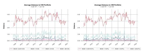
Figure 8 illustrates the L₁ distance between the posterior mean of $\mathit{\nu }$ and ${\mathit{w}}_0$ under the influence of varying c values of 0.001, 1, 5, and 20, noting that the scenario with c = 1 aligns with the parameters of our earlier analysis in this study. As in previous examinations, ${\mathit{w}}_0$ is modeled using a value-weighted portfolio, and the evaluation period and rebalancing frequency remain consistent with our earlier investigations. Importantly, this analysis excludes considerations of risk aversion and transaction costs, concentrating solely on the behavior of unscaled weights.

Figure 8 reveals that increasing MCM deviations lead to a posterior closely resembling the prior, underlining a key advantage of our model. This convergence of the posterior towards ${\mathit{w}}_0$ is consistent with our theoretical findings in Section S.3 of the supplementary material. While our method consistently shrinks towards the prior weights for c = 1, portfolio weights only become very similar to the prior in periods of high turbulence. However, employing a more sensitive MCM measure substantially amplifies the influence of ${\mathit{w}}_0$, enabling our conjugate method to more precisely adapt and mirror outcomes akin to the Black-Litterman model for investors without specific market views, especially under varied market conditions.

5 Conclusion

In conclusion, this paper introduces a novel Bayesian approach for portfolio optimization, employing a conjugate prior with the optimal portfolio weights as one of the parameters. This innovative method facilitates the seamless incorporation of prior information about portfolio weights, offering a distinct edge over other models, including the well-regarded Black-Litterman model. The latter, while effective, often necessitates more elaborate formulations to integrate views on asset returns, as outlined by Black and Litterman (1992).

A significant advantage of our approach is also its inherent automation, primarily facilitated by the incorporation of high-frequency returns and a MCM for hyperparameter specifications. This addition of data not only enriches the model by providing more information for the prior definition but also enables efficient and timely portfolio adjustments in response to market dynamics. Furthermore, the approach adeptly bridges the gap between low-frequency and high-frequency returns, leveraging the strengths of both to enhance portfolio performance.

In the empirical study, portfolios comprising 50 assets in the S&P 500 were evaluated. The new Conjugate HF-VIX VW and Conjugate HF-EPU VW strategies generally outperformed other strategies, including portfolios referred to as Value-Weighted, Equally Weighted, Jeffreys, Ledoit-Wolf Shrinkage, Black-Litterman, Jorion Hyperparameter, and Greyserman Hierarchical, under various risk aversion and transaction cost settings. While the new strategies demonstrated resilience and superior performance during market downturns, such as the 2008 financial crisis and the COVID-19 outbreak, they also showed sensitivity to higher transaction costs.

For future research, it would be worthwhile to explore the performance of the new conjugate method across diverse asset classes, employing varied rebalancing frequencies, high-frequency data intervals, and testing different prior weights. An intriguing and significant avenue for exploration would also involve analyzing international equity markets and experimenting with different MCMs. Moreover, assessing the effectiveness of the conjugate method with high-dimensional portfolios, beyond the 50 assets considered in this study, would offer valuable insights into its adaptability for different market scenarios.

Acknowledgment

The authors would like to thank Professor Atsushi Inoue, the Associate Editor, and two anonymous Reviewers for their constructive comments that greatly improved the quality of this paper. Olha Bodnar acknowledges the support from the internal grant (Rörlig resurs) of the Örebro University. Taras Bodnar acknowledges Vetenskapsrådet (VR) for partly funding his research through the grant “Bayesian Analysis of Optimal Portfolios and Their Risk Measures” (2017-04818).

Notes

¹ We would like to thank Alpha Vantage for providing us with access to high-frequency data.

Table 1 Performance metrics for various strategies employing monthly rebalancing and a portfolio size of 50, for the period January 2007 until July 2023, with risk aversion parameter γ = 5 and transaction cost τ = 15 bps.

	VW	EW	Conjugate HF-VIX VW	Conjugate HF-EPU VW	Jeffreys^1	Shrinkage^1	Jorion Hyperpar.	Black-Litterman	Greyserman Hiera.
Cum. Return	385.919%	344.432%	1947.273%	1071.232%	−100.000%	−100.000%	313.169%	359.423%	54.240%
CAGR	10.058%	9.464%	20.084%	16.087%	NA	NA	8.981%	9.684%	2.662%
Sharpe	0.529	0.508	0.703	0.616	NA	NA	0.397	0.529	0.186
Prob. Sharpe	55.873%	52.529%	80.137%	68.893%	NA	NA	34.856%	55.807%	10.754%
Sortino	0.745	0.715	1.000	0.863	NA	NA	0.558	0.744	0.252
Calmar	0.197	0.180	0.396	0.265	NA	NA	0.108	0.197	0.062
Max. DD	−50.984%	−52.458%	−50.669%	−60.694%	−100.000%	−100.000%	−82.884%	−49.109%	−42.797%
Avg. Loss	−0.866%	−0.830%	−1.481%	−1.371%	−5.370%	−5.889%	−1.945%	−0.824%	−0.639%
Avg. Return	0.046%	0.044%	0.093%	0.077%	−0.417%	−0.731%	0.075%	0.044%	0.015%
Avg. Win	0.789%	0.771%	1.465%	1.331%	3.939%	3.137%	1.853%	0.751%	0.592%
Best Day	10.758%	10.857%	13.233%	11.656%	15.626%	12.677%	26.727%	10.119%	9.935%
Worst Day	−11.415%	−11.367%	−15.365%	−17.805%	−44.144%	−97.182%	−21.820%	−10.814%	−9.018%
Ann. Vol.	20.121%	19.725%	32.020%	30.101%	100.812%	127.257%	45.475%	19.121%	14.902%
Daily VaR	−2.039%	−2.000%	−3.225%	−3.042%	−10.486%	−13.542%	−4.636%	−1.937%	−1.529%
Avg. Turnover	1.432%	4.700%	328.870%	317.087%	542.813%	384.143%	199.890%	1.477%	31.711%

Table 2 Performance metrics for various strategies employing monthly rebalancing and a portfolio size of 50, for the period January 2007 until July 2023, with risk aversion parameter γ = 10 and transaction cost τ = 15 bps.

	VW	EW	Conjugate HF-VIX VW	Conjugate HF-EPU VW	Jeffreys	Shrinkage	Jorion Hyperpar.	Black-Litterman	Greyserman Hiera.
Cum. Return	385.919%	344.432%	536.701%	376.358%	17.141%	204.414%	213.037%	359.423%	40.097%
CAGR	10.058%	9.464%	11.876%	9.925%	0.964%	6.981%	7.163%	9.684%	2.065%
Sharpe	0.529	0.508	0.726	0.648	0.282	0.358	0.379	0.529	0.183
Prob. Sharpe	55.873%	52.529%	82.653%	73.381%	19.703%	29.283%	32.303%	55.807%	10.516%
Sortino	0.745	0.715	1.035	0.913	0.394	0.502	0.528	0.744	0.246
Calmar	0.197	0.180	0.421	0.325	0.010	0.084	0.139	0.197	0.092
Max. DD	−50.984%	−52.458%	−28.223%	−30.499%	−94.470%	−82.630%	−51.513%	−49.109%	−22.488%
Avg. Loss	−0.866%	−0.830%	−0.739%	−0.681%	−2.494%	−2.042%	−0.967%	−0.824%	−0.319%
Avg. Return	0.046%	0.044%	0.050%	0.042%	0.067%	0.070%	0.037%	0.044%	0.009%
Avg. Win	0.789%	0.771%	0.734%	0.666%	2.391%	1.944%	0.917%	0.751%	0.294%
Best Day	10.758%	10.857%	5.097%	4.792%	34.501%	28.420%	12.692%	10.119%	4.259%
Worst Day	−11.415%	−11.367%	−7.896%	−8.563%	−27.120%	−22.129%	−11.651%	−10.814%	−4.761%
Ann. Vol.	20.121%	19.725%	15.872%	14.819%	55.971%	46.323%	22.256%	19.121%	7.355%
Daily VaR	−2.039%	−2.000%	−1.595%	−1.493%	−5.733%	−4.730%	−2.269%	−1.937%	−0.753%
Avg. Turnover	1.432%	4.700%	163.542%	157.347%	278.558%	189.671%	93.270%	1.477%	15.637%

Figure 1 Illustration of S&P 500 cumulative returns alongside VIX and EPU indices from January 2007 to July 2023.

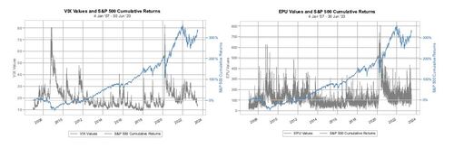
Figure 2 Visual representation of performance for various strategies employing monthly rebalancing and a portfolio size of 50, for the period January 2007 until July 2023, with risk aversion parameter γ = 5 and transaction cost τ = 15 bps.

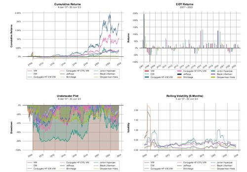
Figure 3 Maximum long and short positions for various strategies employing monthly rebalancing and a portfolio size of 50, for the period January 2007 until July 2023, with a risk aversion parameter of γ = 5 and a transaction cost of τ = 15 bps.

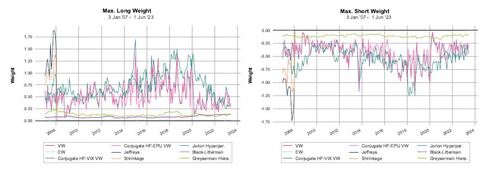
Figure 4 Sharpe ratio and CAGR for various strategies employing monthly rebalancing and a portfolio size of 50, for the period January 2007 until July 2023, with a risk aversion parameter of γ = 5 and at different transaction cost levels.

Figure 5 Visual representation of performance for various strategies employing monthly rebalancing and a portfolio size of 50, for the period January 2007 until July 2023, with risk aversion parameter γ = 10 and transaction cost τ = 15 bps.

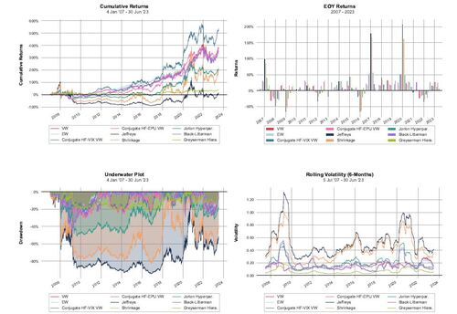
Figure 6 Maximum long and short positions across various strategies employing monthly rebalancing and a portfolio size of 50, for the period January 2007 until July 2023, with a risk aversion parameter of γ = 10 and a transaction cost of τ = 15 bps.

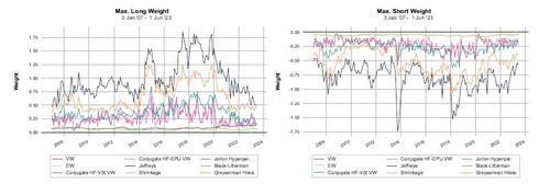
Figure 7 Sharpe ratio and CAGR for various strategies employing monthly rebalancing and a portfolio size of 50, for the period January 2007 until July 2023, with a risk aversion parameter of γ = 10 and at different transaction cost levels.

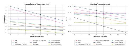
Figure 8 L₁ distance between the posterior mean of $\mathit{\nu }$ and ${\mathit{w}}_0$ using the conjugate method with different MCM scaling factors, employing monthly rebalancing and a portfolio size of 50, for the period January 2007 until July 2023.