Performance evaluation of a multi-product system under CONWIP control

Abstract

Analytical models of multi-product manufacturing systems operating under CONWIP control are composed of closed queuing networks with synchronization stations. Under general assumptions, these queuing networks are hard to analyze exactly and therefore approximation methods must be used for performance evaluation. This research proposes a new approach based on parametric decomposition. Two-moment approximations are used to estimate the performance measures at individual stations. Subsequently, the traffic process parameters at the different stations are linked using stochastic transformation equations. The resulting set of non-linear equations is solved using an iterative algorithm to obtain estimates of key performance measures such as throughput, and mean queue lengths. Numerical studies indicate that the proposed method is computationally efficient and yields fairly accurate results when compared to simulation.

Keywords:

• Multi-product systems
• CONWIP
• pull systems
• closed queuing network
• fork/join stations
• parametric decomposition
• two-moment approximations

1. Background and literature review

Manufacturing industries are under increasing pressure to offer a large variety of products to their customers with shorter lead times and at reduced costs. This has led to a significant interest in pull-type material control systems and their ability to improve factory efficiencies. The CONWIP system proposed by Spearman et al. (1990) is one of the simplest ways to implement pull control. Unlike traditional kanban systems that impose limits on inventory at each manufacturing stage, the CONWIP system uses kanban cards to solely limit the overall inventory in the system (Work In Process (WIP) as well as finished goods inventory). The superiority of the CONWIP system over traditional kanban systems has been argued in several papers including Spearman (1992) and Spearman and Zazanis (1992). Performance comparisons of CONWIP with other systems have been reported in Buzacott and Shanthikumar (1993) and Bonvik et al. (2000). A majority of these efforts focus on manufacturing systems with a single product. Recently, there has been significant interest in understanding the impact of WIP limits in multi-product CONWIP systems. Studies such as Duenyas (1994). Ryan et al. (2000) and Ryan and Vorasayan (2005) argue that when product characteristics (such as routing and processing time requirements) are different, imposing product-specific WIP limits (using dedicated kanbans to individual products) is better than imposing an overall WIP limit (using shared kanbans). However, determining the WIP limits appropriate for individual products requires understanding the complex dynamics of manufacturing systems. The queuing models described in this paper can be used to analyze the impact of WIP limits on performance measures such as throughput, inventory and backorders.

Queuing network models of multi-product manufacturing systems operating under CONWIP control are comprised of multi-class closed networks with fork/join synchronization stations. When the manufacturing system has fairly general characteristics (such as product-specific routings and distinct processing times for each product at the different stations), exact analysis of the underlying queuing network can be very hard. Consequently approximation methods have been used for performance evaluation. Ryan and Choobineh (2003) and Ryan and Vorasayan (2005) use non-linear programming formulations to determine WIP limits that guarantee desired throughput levels for individual products. Hopp and Roof (1998) use statistical throughput control to analyze CONWIP systems, and Baynat and Dallery (1996) use product-form approximations to estimate the performance measures of interest.

This paper proposes a new approach based on parametric decomposition. The approach is based on characterizing the traffic processes (arrival and departure) in the network using mean and variability parameters. Two-moment approximations are used to estimate the performance measures at individual stations, and the traffic process parameters at the different stations are linked using suitable stochastic transformation equations. These result in a set of non-linear equations that is solved to estimate the performance measures of interest. Although the parametric decomposition technique has been extensively used for the analysis of open queuing networks (see Whitt (1983, 1994) and Bitran and Tirupati (1988) and the references therein), its use in the analysis of closed queuing networks has been limited. Kamath et al. (1988) use a parametric-decomposition-based approach to analyze a single-class cyclic network, while more recently, Krishnamurthy and Suri (2006) use a parametric-decomposition-based approach to analyze single-class closed networks with synchronization stations. The key challenge in extending the approach to multi-class networks, is to efficiently model the interactions of the multiple classes while determining performance measures for each class of customers. In this paper, new approximations are derived for the mean waiting times of customers of individual classes at the different stations of the network. These approximations are subsequently used in an iterative procedure that yields the key performance measures of interest. A key feature of this approach is that it can be easily used to study of the effects of variability in multi-product CONWIP systems.

The rest of the paper is organized as follows. Section 2 describes the queuing model of the multi-product system operating under CONWIP control. Section 3 describes the approach used for the analysis of the network. The details of the analysis are discussed in individual subsections. Section 4 summarizes the results of the numerical studies conducted to test the approach, and Section 5 summarizes the conclusions and possible extensions of this research.

2. System model

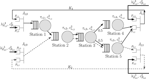
This section describes the queuing network model of a multi-product system with R products (labeled r = 1, …, R) and M manufacturing stations (labeled m = 1, …, M) operating under CONWIP control. It is assumed that the kanban cards are specific to each product, and that there are K _r cards for product r. Each manufacturing station is modeled as a single server queue operating under a first-come first-served service discipline. The service time distribution of a product r at a manufacturing station m is described by two parameters: the mean, τ _r,m , and the Squared Coefficient of Variation (SCV), c _r,m ². Note that a mean service time of τ _r,m implies that the service rate, μ _r,m for product r at station m is equal to τ⁻¹ _r,m . Fork/join stations are used to model synchronization constraints between: (i) raw materials and CONWIP cards; and (ii) finished goods and customer demands respectively. Each product route has two fork/join stations, J _r,i , i = 0, 1 and each fork/join station, J _r,i , has two input buffers, P _r,i and F _r,i+1. Figure 1 illustrates a system with M = 5 and R = 2. The system operates as follows.

Raw materials of product r arrive at buffer P _r,0 of the fork/join station J _r,0. The raw material arrival process is described by two parameters, namely the mean, λ _{P r,0} ⁻¹, and the SCV, c _{P r,0} ², of the inter-arrival times. It is assumed that at most K _r,0 units of raw materials of product r can queue in buffer P _r,0 at any point in time. Free CONWIP cards corresponding to product r queue at the buffer F _r,1 of the fork/join station J _r,0. When there is at least one unit of raw material in the buffer P _r,0 and one free CONWIP card in the buffer F _r,1, one entity from each buffer is removed and “joined” to form a combined entity. This combined entity is released to the first manufacturing station in the product's routing.

In the manufacturing system, product r undergoes processing at each station in its routing. The routing for each product r is defined by its routing matrix B _r , whose elements b _{r i,j} denote the probability that product r visits station j upon completion of service at station i. B _r is a (M+2)× (M+2) matrix, with the indices i = 0 and i = M+1 in b _{r i,j} denoting the upstream fork/join station J _r,0, and the downstream fork/join station J _r,1, respectively. For simplicity of exposition, it is assumed that the elements b _{r i,j} are such that each product undergoes processing at a manufacturing station at most once, and that b _{r 0,j} = 1 and b _{r i,M+1} = 1 for some j and i respectively. The method described here can be extended to the case where these assumptions on the routing are relaxed. Note that the routing matrices can be used to define a set V _r comprised of the indexes of the manufacturing stations visited by product r, and a set E _m comprised of the indices of the products processed at manufacturing station m.

After completing processing at the last manufacturing station in its route, product r is routed to fork/join station J _r,1 where it queues in the finished goods buffer, P _r,1 to get matched with a customer demand for that product. Customer demands for product r arrive to buffer F _r,2 of station J _r,1. The demand arrival process of product r is described by two parameters, namely the mean, λ _{F r,2} ⁻¹, and SCV, c _{F r,2} ², of the demand inter-arrival times. Furthermore, it is assumed that at most K _r,1 customer demands for product r can queue in buffer F _r,2 at any point in time. At the station J _r,1, customer demands in buffer F _r,2 and finished products in buffer P _r,1 “join” together and exit the system. At the same instant, the CONWIP card attached to the finished product is released and “forks” back to buffer F _r,1 to enable the release of another unit of product r into the system. Note that customer demands waiting in buffer F _r,2 and products waiting in buffer P _r,1 correspond to backorders and finished goods inventory, respectively. In Fig. 1, product 1 has a probabilistic routing described by b _10,1 = b _11,2 = b _12,3 = b _14,6 = b _15,6 = 1 and b _13,4 = b _13,5 = 0.5, while product 2 has a deterministic routing described by b _20,2 = b _22,3 = b _23,5 = b _15,6 = 1. For this network E ₁ = (1), E ₂ = (1,2), E ₃ = (1,2), E ₄ = (1), E ₅ = (1,2) and V ₁ = (1,2,3,4,5), V ₁ = (2,3,5).

Fig. 1 Queuing model of multi-product CONWIP system.

3. Overall approach and analysis details

The overall approach is based on parametric decomposition. It has two main features. First, it approximates the traffic processes (arrival and departure processes at the different stations) in the network by renewal processes, and second, it characterizes the distribution of the inter-renewal times of the renewal processes by two parameters, namely the mean and the SCV. In reality, the arrival and departure processes in the network are not renewal. Therefore, the two-parameter characterization is an approximate representation of these traffic processes by “equivalent” renewal processes. The first parameter, corresponding to the mean, is equal to the mean of the corresponding inter-arrival or inter-departure times. The role of the second parameter, corresponding to the SCV of the equivalent renewal process is to account for the complex structure of the arrival and departure processes in an aggregate way. When applied to the analysis of closed queuing networks such as that shown in Fig. 1, the approach consists of four steps.

1.	Decomposition. Decomposition of the network yields M manufacturing stations and 2R synchronization stations. Note that, each manufacturing station, m (m = 1,…, M), could serve multiple products, but each synchronization station, J r,i , i = 0,1, is dedicated to product r.
2.	Characterization. Each station obtained from decomposition is analyzed under the assumption that the arrival and service processes at the station are renewal processes characterized by two parameters, the mean and SCV of the inter-renewal times. While the parameters characterizing the service process at the manufacturing station m, and external raw material (at J r,0) and demand arrival processes (at J r,1) are known inputs for the analysis, the parameters characterizing the internal traffic processes in the network are not known. In the characterization step, it is assumed that the two parameters characterizing the arrival process at each station are also known. Using this information, each station is analyzed in isolation to obtain two-moment approximations that describe the departure process and the performance measures at the station. For details see Section 3.1 and 3.2.
3.	Linkage. In this step, the traffic processes at the individual stations are linked together using two key features of the closed queuing network. First, with respect to station m, it is noted that the arrival process is the superposition of the departure process of different products from the preceding station. Second, with respect to product r, it is noted that the sum of the mean queue lengths at the different manufacturing stations and the synchronization stations J r,i in its route for each product r must be equal to its population constraint, K r . Using these facts, expressions that link the mean and SCV parameters of the arrival and departure processes at the different stations are derived. This results in a system of non-linear equations. For details see Section 3.3.
4.	Solution. The system of non-linear equations is solved using an iterative algorithm to determine the unknown parameters characterizing the internal traffic processes. Once these parameters are obtained, the network performance measures such as the system throughput and mean queue lengths at the different stations can be easily computed. For details see Section 34.

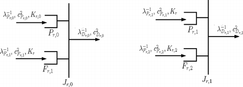
3.1. Characterization of fork/join synchronization stations J _r,i .

Figure 2 shows the fork/join synchronization stations, J _r,0 and J _r,1, obtained from the decomposition step. Raw material arrivals to buffer P _r,0 at J _r,0 are characterized in terms of the mean and SCV (λ _{P r,0} ⁻¹ and c _{P r,0} ²) of the inter-arrival times, and K _r,0, the maximum number of raw material units permitted to queue at P _r,0. Similarly, arrivals of free cards to buffer F _r,1 at J _r,0 are characterized in terms of the mean and SCV of the inter-arrival times (λ _{F r,1} ⁻¹ and c _{F r,1} ²) and K _r , the number of kanban cards for product r. The arrival process of free cards from the rest of the network to buffer F _r,1 shuts down when all K _r cards are in the buffer. This implies that the input to the station J _r,0 is characterized by the parameter six-tuple (λ _{P r,0} , c _{P r,0} ², K _r,0,λ _{F r,1} , c _{F r,1} ², K _r ). Similarly, the input to the station J _r,1 is characterized by the parameter six-tuple (λ _{P r,1} , c _{P r,1} ², K _r ,λ _{F r,2} , c _{F r,2} ², K _r,2). Krishnamurthy et al. (2003) and Krishnamurthy and Suri (2006) analyze fork/join stations characterized by the input tuple (λ _{P r,i} , c _{P r,i} ², K _r,i ,λ _{F r,i+1} , c _{F r,i+1} ², K _r,i+1) and derive expressions for the mean (λ⁻¹ _{D r,i} ) and SCV (c _{D r,i} ²) of the inter-departure times, and the mean queue lengths ( _{P r,i} and _{F r,i+1} ) at the buffers (P _r,i and F _r,i+1). Those results are used as characterization equations for the fork/join stations. For notational simplicity, the following parameters are defined:

The expressions for the performance measures are if w _r,i ≠1:

Fig. 2 Characterization of fork/join synchronization stations J _r,i .

if w _r,i = 1

For the system discussed in this paper, the characterization equations for upstream fork/join station J _r,0 are obtained by setting i = 0, and K _r,1 = K _r in the above equations. Similarly, setting i = 1, and K _r,1 = K _r yields the equations for downstream fork/join station J _r,1.

3.2. Characterization of manufacturing stations

Figure 3 shows a manufacturing station m obtained from the decomposition step. It is assumed that the inter-arrival times of product r at station m are characterized by their mean and SCV (λ_{a r,m} ⁻¹ and c _{a r,m} ²). Similarly, the service times for product r at station m are characterized by their mean and SCV (τ _r,m and c _{s r,m} ²). In the characterization step, expressions for the mean and SCV (λ_{d r,m} ⁻¹ and c _{d r,m} ²) of the inter-departure times and mean queue length ( _r,m ) are written. The details are presented in the following subsections.

Fig. 3 Characterization of manufacturing station m.

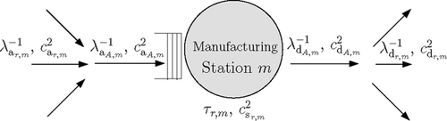
3.2.1. Analysis of departure process

Note that the arrivals to a manufacturing station m is actually the superposition of the arrival processes of the products routed through the station. First, using superposition arguments an aggregate product is defined at station m. Then, the departure process at station m is characterized using the mean and SCV parameters (λ_{a A,m} ⁻¹, c _{a A,m} ²) of the inter-arrival times, and the mean and SCV parameters (τ _A,m and c _{s A,m} ²) of the service time of this aggregate product. (Note that throughout this discussion, the subscript A is introduced to emphasize parameters of the aggregate product.) The analysis in Whitt (1983) and Bitran and Tirupati (1988) yield Equations (13)–(16) for these parameters. In particular:

where φ _r,m = λ_{a r,m} /λ_{a A,m} for all r∈ E _m . If ρ _r,m denotes the utilization of a manufacturing station m due to a product r, then ρ _r,m is equal to λ_{a r,m} τ _r,m for all r∈ E _m and the overall station utilization ρ _m is given by ρ _m = λ_{a A,m} τ _A,m (= ∑ _{r ∈ E m} ρ _r,m ). Additionally, expressions for c _{a A,m} ² and c _{s A,m} ² are written as

where ω⁻¹ = [1+4(1−ρ _m )²(ν−1)], c ² = ∑ _{r = 1} ^R φ _r,m c _{a r,m} ² and ν⁻¹ = ∑ _{r = 1} ^R φ _r,m ². In terms of these input parameters, expressions for the mean, λ⁻¹ _{d A,m} , and SCV, c _{d A,m} ², of the inter-departure times are written as follows:

Finally, expressions characterizing the mean and SCV parameters (λ _{d r,m} and c _{d r,m} ²) of the inter-departure times for an individual product r routed through station m are written as

If the routing for product r is not deterministic, it is possible that subsequent to departure from station m, product r is not routed to a unique station. Instead, it could be routed to a particular station j among several possible stations with probability b _{r m,j} , with 0 < b _{r m,j} < 1. In this case, the mean and SCV parameters characterizing the departures of product r from station m to station j are written in terms of λ_{d r,m} , c _{d r,m} ², and the routing probability b _{r m,j} using equations provided in Whitt (1983; Section 4.4). Subsequently, at each station j, the parameters of the aggregate product at station j are computed as discussed earlier in this section and the departure process is analyzed in terms of this aggregate product.

3.2.2. Analysis of mean queue length

Let _{q r,m} denote the mean waiting time in queue at a manufacturing station m for product r. Expressions for the mean queue length, _r,m , of a product r, and the overall mean queue length, _m , can be written as

The above equations imply that estimates of the mean waiting times, _{q r,m} , are required to determine the mean queue lengths at station m. However, estimation of _{q r,m} is not straightforward as station m is part of a closed queuing network. If station m were part of an open network, then _qr,m can be considered to be the same for all products and set equal to _q,m ^GI/G/1, the mean waiting time in a GI/G/1 queue characterized by the parameters for the aggregate product i.e., λ_{a A,m} , τ _A,m , c _{s A,m} ² and c _{a A,m} ². Although the expression is not exact, Whitt (1983) argues that this estimate is often accurate enough for analysis purposes. However, since station m is a part of a closed queuing network, _{q r,m} would be a function of λ_{a r,m} , τ _r,m , c _{s r,m} ², c _{a r,m} ² and K _r of all the r products at each station, that is

Estimating this functional relationship, g can be extremely hard for a general non-product-form closed queuing network, such as the one under consideration. Therefore, the mean waiting time is written as a product of two terms, _q,m ^GI/G/1 and f _r,m . The second term f _r,m , in an approximate way, accounts for the impact of the finite populations of the different products on the mean waiting time of product r at station m. Therefore, _q,m is written as

The next section describes the determination of f _r,m .

3.2.3. Determination of f _r,m

To determine the f _r,m , corresponding to each class in the original multi-class closed queuing network, R single-class product-form closed queuing networks, C ^(r), r = 1, …, R are defined. The stations in C ^(r) correspond to the manufacturing stations and the fork/join stations, J _r,0 and J _r,1, in the routing for product r. Product r is routed through stations in C ^(r) according to its routing matrix B _r . To ensure that C ^(r) has a product-form solution, the following two assumptions are made: one with respect to manufacturing stations, and the other with respect to the fork/join stations.

With respect to the manufacturing stations in C ^(r), it is assumed that the service times are exponentially distributed. Additionally, the effect of the other products, r′ ≠ r, are accounted for in an aggregate way using the following argument. From the perspective of a unit of product r waiting in the queue at station m, it is assumed that the station is temporarily unavailable whenever it is processing products of type r′≠ r that are ahead of it in the queue. The effect of server unavailability on product r is accounted for by artificially inflating the mean service times, _r,m of product r at station m in the network C ^(r) by a suitable factor. Since the proportion of time that station m is unavailable for product r is ∑ _{k∈ E m , k≠ r} ρ _k,m , the mean service time _r,m , is given by

Equation (25) ensures that the effective capacity of station m in the network C ^(r) is equal to the the effective capacity of station m for product r in the original network.

Corresponding to the fork/join stations, J _r,0 and J _r,1, in the original network, two stations with exponential service times are defined. These stations are defined such that the mean queue length of kanbans (the customers in the closed network) at these stations in C ^(r) are approximately equal to the mean queue lengths at the corresponding buffers of the fork/join stations in the original network. At station J _r,0, if w _r,0 = 1 it is replaced by a station with infinite servers, with each server having a mean service time of λ⁻¹ _{D r,0}(K _r,1/2) (K _r,1+1)/( _r,0+1). Note that Equation (12) implies that when w _r,0 = 1, the mean queue length at this infinite server station in C ^(r) would be exactly equal to the mean queue length at buffer F _r,1 in the original network. If w _r,0≠ 1, it could be argued that free kanbans primarily wait for raw materials and therefore, the fork/join station J _r,0 is replaced by a single exponential server station with mean service time, λ _{P r,0} ⁻¹. Similarly, at station J _r,1, if w _r,1 = 1 it is replaced by a station with infinite servers, with each server having a mean service time of λ⁻¹ _{D r,1}(K _r,1/2) (K _r,1+1)/( _r,1+1). Again, Equation (11) implies that the mean queue length at this infinite server station in C ^(r) would be exactly equal to the mean queue length at buffer P _r,1 in the original network. When w _r,1≠ 1 the fork/join station J _r,1 is replaced by a single exponential server with mean service time, λ _{F r,2} ⁻¹. The equivalent single-class networks are shown in Fig. 4.

Fig. 4 Equivalent single-class networks defined for determination of f _r,m .

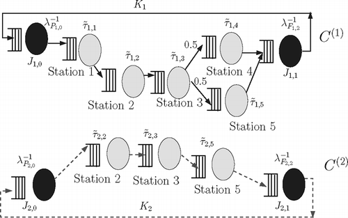
Under these assumptions, network C ^(r) has a product form solution that can be obtained using a suitable method such as a convolution algorithm or Mean Value Analysis to determine performance measures such as the throughput, _r,m , and the mean waiting time, [Wtilde] ^C(r) _{q r,m} , at each station m in C ^(r). Next, consider an M/M/1 queue with arrival rate equal to the throughput of the network C ^(r), _r,m and exponential service times with mean, _r,m . Let [Wtilde] ^O _{q r,m} be the mean waiting time in this M/M/1 queue. Then, f _r,m is defined as the ratio of the mean waiting time in C ^(r) to the mean waiting time in the M/M/1 queue. Therefore, f _r,m is written as

Note that the expression for f _r,m derived in Equation (26) above implies:

Substituting the expression for _{q r,m} in Equation (21) and Equation (22), the mean queue lengths, _r,m and _m at each station m in the original network are obtained. By expressing the mean waiting times in Equation (27) as a product of the three terms ^GI/G/1 _q,m , [Wtilde] ^O _{q r,m} and [Wtilde] ^{C, (r)} _{q r,m} , estimates of the mean queue length are obtained without excessive computations. Both the terms, ^GI/G/1 _q,m and [Wtilde] ^O _{q r,m} , are simple analytical expressions, while the term, [Wtilde] ^{C, (r)} _{q r,m} , requires the solution of a relatively simple single-class product-form closed queuing network. Finally, note that in order to determine the service times in the single-class closed queuing network, C ^(r) estimates of the arrival rates λ_{a r,m} are required. As mentioned earlier, these estimates are assumed to be known at the characterization step, and are estimated in the linkage and solution steps of the overall approach. The details of these steps are discussed next.

3.3. Linkage

In the characterization step, the parameters describing the inputs at manufacturing and synchronization stations were assumed to be given, when in fact the parameters characterizing the internal traffic flows need to be determined. This section describes how the equations used to determine these parameters are established for each product r.

Note that the station preceding a manufacturing station j, j ∈ V _r , could be either the fork/join station J _r,0 (if station j is the first station in the routing for product r) or another manufacturing station i. If station j is preceded by a fork/join station then the departure process parameters at J _r,0, (λ _{D r,0} ,c _{D r,0} ²) are equated to the arrival process parameters (λ_{a r,j} ,c _{a r,j} ²) at station j. If station j is preceded by other manufacturing stations i, i ∈ V _r , then the departure process parameters (λ_{d r,i} ,c _{d r,i} ²) at station i are related to the arrival process parameters (λ_{a r,j} ,c _{a r,j} ²) at station j using the routing probabilities, b _{r i,j} . Since the specific linking equations are identical to those specified in Krishnamurthy and Suri (2006, Section 4.3) and Whitt (1983, Section 4.4), the details of these equations are omitted here.

Next, consider arrivals to fork/join stations J _r,0 and J _r,1 in the routing for product r. Note that, in the routing for product r, station J _r,0 is preceded by station J _r,1. Therefore, the parameters describing the departure process of free cards at J _r,1 (i.e., λ _{D r,1} , c _{D r,1} ²) need to be related to the parameters describing the arrival process of free cards at buffer F _r,1 (i.e., λ _{a r,j} , c _{a r,j} ²) at station J _r,0. Unlike station J _r,0, station J _r,1 is preceded by a manufacturing station (say station i). This implies that the linking equations need to relate the parameters describing the departure process of product r at station i (i.e., λ_{d r,i} , c _{d r,i} ²) to the parameters describing the arrival process of product r at buffer P _r,1 (i.e., λ _{P r,1} , c _{P r,1} ²) at station J _r,1. The specific linking equations are identical to those specified in Krishnamurthy and Suri (2006, Section 4.3) and the details of these equations are omitted here.

Finally, it is noted that since the system operates under CONWIP control, for each product r, the queue lengths at individual stations should sum up to K _r , implying that the following relationship must hold:

The above linking relationships yield a system of non-linear equations in terms of the mean and SCV parameters characterizing the internal traffic processes of each product r. The solution algorithm described in the next section solves this system of equations.

3.4. Solution

The solution algorithm begins with an initial vector, Λ ⁽⁰⁾ = (λ₁,…, λ _R ) of throughput estimates and progressively updates the estimates of throughput and different traffic process parameters until they converge (within a user-specified tolerance limit) and are consistent with the input parameters. To improve the efficiency of the algorithm, the search for each λ _r is restricted to be between lower and upper bounds, λ _r ^LB and λ _r ^UB. The lower bound, λ _r ^LB, is set equal to zero. The upper bound, λ _r ^UB, is set noting that the throughput, λ _r , for each product r in the closed queuing network must be less than min _{m ∈ V(r)}(λ _{P r,0} , μ _r,m , λ _{F r,2} ). The other inputs to the algorithm are the product routing matrices B _r , service time parameters μ _r,m , c ² _{s r,m} , ∀ r ∈ V _r , and the population limits K _r , K _r,0 and K _r,2 respectively. The details of the algorithm are provided below. The description assumes that all products are routed sequentially through all M stations. The procedure only requires minor modifications if this is not the case.

In Step 1, the algorithm sets the initial throughput estimates to be equal to the lower bounds. The iterative procedure starts by equating the initial throughput estimate, λ _r , to the arrival rate, λ_{a r,1} , at station 1 for each product r. To completely specify the arrival process at station 1, an initial choice of c _{a r,i} ² is also made. However, the initial choice of λ_{a r,1} and c _{a r,1} ² might not be consistent with each other. Therefore, in Step 2, the algorithm updates the initial estimate of c _{a r,1} ² till it is consistent with the current choice of λ_{a r,1} . To update the estimate of c _{a r,1} ², the algorithm uses the linking and characterization equations derived in the previous sections successively at each station in the routing for product r. Subsequently, the departure process parameters at J _r,1 and J _r,0 are estimated. Since departures from J _r,0 form arrivals to station 1, a new estimate of c _{a r,1} ² is obtained. If the old and the new estimates of c _{a r,1} ² are not within a pre-defined tolerance limit, the procedure is repeated for each product r with the new estimate of c _{a r,1} ². Once the algorithm obtains a value of c _{a r,1} ² which is consistent with the choice of λ_{a r,1} , in Step 3 the algorithm verifies whether the values of λ_{a r,1} and c _{a r,1} ² are consistent with the other input parameters of the network. In particular, the algorithm verifies whether the sum of the mean queue lengths at stations in V _r sums up to K _r for each product r (Equation (28)). If Equation (28) is satisfied within some user-specified tolerance limit, the algorithm terminates. Otherwise in Step 4, the choice of (λ₁,…, λ _R ) must be updated. Broyden's method (Broyden, 1965) is used to determine a new estimate Λ^(new) = (λ^(new) ₁,…, λ^(new) _R ). Using this new vector, Steps 2 and 3 are repeated.

Solution algorithm

Given: K _r , K _r,0, K _r,2, μ _r,m , c _{s r,m} ², ∀ r, m

Define: Δ _r = | _r −K _r | and Δ = max _r (Δ _r ); calculate the λ _r ^LB, λ _r ^UB

	Step 1. Initialize: Λ(0) = (λ1 LB , …,λ R LB ), Δ = 1.0 Step 2. While |Δ| > ε1 do 2.1 Initialize c a r,1 2 = min m (c s r,m 2)∀ r, δ = 1 2.2 While |δ| > ε2 do Compute c d r,m 2, c a r,m 2, c D r,0 2, c D r,1 2 ∀, r, m from characterization and linkage equations, compute δ = max r |c a r,1 2−c dr,M 2| and set c a r,1 2 = c d r,M 2∀ r
	Step 3. Compute mean queue lengths r,m , P r,0 , P r,1 , r ∀ r, ∀ m. This requires solving the R single class networks to compute f r,m for each r,m. Verify if Equation (28) is satisfied. If Δ = max r (Δ r ), then STOP. Else proceed to Step 4.
	Step 4. Calculate new estimates of Λ (new) = (λ1 (new), …, λ R (new)) using Broyden's method.

4. Numerical results

To check the numerical accuracy of the proposed method, the algorithm was implemented in MATLAB (Rev 6.5.1) and executed on an Intel Pentium IV PC. The algorithm converged to yield performance estimates in less than a minute for each scenario (when ε₁ = ε₂ = 0.01). The results from the analytical model were compared with those obtained from a simulation model built using ProModel (www.promodel.com) and executed on the same PC. The simulation experiment for each scenario took 10 minutes on average. The simulation results were recorded based on five independent simulation runs with a 95% confidence interval. This ensured that the standard deviation of the throughput value from different replications is within ± 0.5 % of the mean. Each run represented the production of at least 200 000 parts. The statistics corresponding to first 50 000 parts were discarded to account for the transient start-up effects. In all the simulation experiments, the random variables corresponding to service times, raw material and demand inter-arrival times were generated using samples from a two-phase Coxian distribution with balanced means. The main performance measures recorded in all experiments were the throughput (λ _r ) and the mean queue lengths at the manufacturing and fork/join stations ( _r,m , _{F r,i} and _{P r,i} ) for each product. To determine the numerical accuracy of the proposed analytical approach, percentage errors between the analytical estimate (A) and the simulation estimate (S) of the performance measures were computed. The percentage errors in throughput and mean queue lengths are computed as

The error in the queue length was computed as a percentage of the total number of customers for product r to avoid the potential problems that might arise when the average queue length itself is small. Next, results from three sets of experiments are reported.

4.1. Experiment 1

In this experiment, the performance of a network with R = 3 products and M = 3 manufacturing stations is analyzed. The products have identical routing, and each product r visits manufacturing stations m = 1, 2 and 3 sequentially. Table 1 shows the input settings and corresponding outputs for eight different cases (labeled 1–8). In all cases μ _r,m = 6 for all r,m; λ _{P r,0} = 6 and K _r,0 = K _r,2 = 4 for all r. The results for the eight cases provide insights regarding the impact of different input parameters such as card limits (K _r ), demand arrival rates (λ _{F r,2} ) and SCVs (c _{P r,0} ², c _{F r,2} ², c _{s r,m} ²) on important performance measures such as throughput (λ _r ), mean queue lengths ( _r,m ) and average backorders ( _{F r,2} ) for each product.

Table 1 Results for Experiment 1: results are shown for the case where μ _r,m = 6, ∀ r,m; K _r,0 = K _r,2 = 4; λ _{P r,0} = 6

					Throughput			Mean queue length									Backorders
	(K r , K 2, K 3)	λ F r,2	c P r,0 ^2 = c F r,2 ^2 = c s r,m ^2		λ1	λ2	λ3	1,1	2,1	3,1	1,2	2,2	3,2	1,3	2,3	3,3	F 1,2	F 2,2	F 3,2
1	(4, 4, 4)	1.5	0.7	A	1.486	1.486	1.486	0.486	0.486	0.486	0.493	0.493	0.493	0.496	0.496	0.496	0.332	0.332	0.332
				S	1.490	1.491	1.495	0.678	0.678	0.680	0.687	0.686	0.688	0.696	0.696	0.697	0.185	0.180	0.185
				E	−0.271	−0.309	−0.613	−4.800	−4.800	−4.850	−4.850	−4.825	−4.875	−5.000	−5.000	−5.025	3.687	3.804	3.687
2	(4, 4, 4)	1.5	2	A	1.413	1.413	1.413	0.676	0.676	0.676	0.739	0.739	0.739	0.770	0.770	0.770	0.982	0.982	0.982
				S	1.360	1.370	1.371	0.678	0.678	0.680	0.687	0.686	0.688	0.696	0.696	0.697	0.916	0.915	0.917
				E	3.884	3.076	3.037	−0.050	−0.050	−0.100	1.300	1.325	1.275	1.850	1.850	1.825	1.652	1.683	1.616
3	(4, 4, 4)	1.75	1	A	1.633	1.633	1.633	0.785	0.785	0.785	0.847	0.847	0.847	0.868	0.868	0.868	1.118	1.118	1.118
				S	1.620	1.622	1.618	1.015	1.017	1.015	1.054	1.053	1.052	1.076	1.078	1.076	0.999	0.994	0.989
				E	0.837	0.683	0.970	−5.750	−5.800	−5.750	−5.175	−5.150	−5.125	−5.200	−5.250	−5.200	2.964	3.093	3.031
4	(4, 4, 4)	1.75	2	A	1.520	1.520	1.520	0.874	0.874	0.874	0.979	0.979	0.979	1.023	1.023	1.023	1.557	1.557	1.557
				S	1.458	1.455	1.458	1.028	1.028	1.029	1.071	1.070	1.072	1.085	1.085	1.086	1.437	1.435	1.452
				E	4.220	4.434	4.238	−3.850	−3.850	−3.875	−2.300	−2.275	−2.325	−1.550	−1.550	−1.575	2.998	3.049	2.633
5	(4, 4, 4)	2	0.7	A	1.761	1.761	1.761	0.935	0.935	0.935	1.025	1.025	1.025	1.045	1.045	1.045	1.519	1.519	1.519
				S	1.760	1.758	1.761	1.210	1.209	1.211	1.233	1.234	1.234	1.238	1.238	1.239	1.603	1.619	1.607
				E	0.064	0.169	0.001	−6.875	−6.850	−6.900	−5.200	−5.225	−5.225	−4.825	−4.825	−4.850	−2.097	−2.512	−2.209
6	(4, 6, 5)	2	0.7	A	1.669	1.882	1.808	1.015	1.144	1.100	1.115	1.257	1.208	1.136	1.280	1.230	1.826	0.917	1.302
				S	1.611	1.931	1.825	1.245	1.539	1.433	1.276	1.583	1.474	1.283	1.601	1.486	2.089	0.675	1.265
				E	3.621	−2.541	−0.926	−5.750	−6.583	−6.660	−4.025	−5.433	−5.320	−3.675	−5.350	−5.120	−6.587	6.040	0.915
7	(3, 3, 3)	6	2	A	1.563	1.563	1.563	0.915	0.915	0.915	1.020	1.020	1.020	1.061	1.061	1.061	3.692	3.692	3.692
				S	1.466	1.466	1.466	0.996	0.997	0.996	1.000	1.000	1.001	1.004	1.002	1.002	3.667	3.664	3.664
				E	6.585	6.585	6.585	−2.700	−2.733	−2.700	0.667	0.667	0.633	1.900	1.967	1.967	0.635	0.691	0.709
8	(4, 6, 5)	6	2	A	1.336	2.002	1.670	1.236	1.852	1.545	1.359	2.036	1.698	1.396	2.092	1.745	3.732	3.601	3.652
				S	1.296	1.944	1.620	1.335	2.001	1.667	1.329	1.994	1.663	1.336	2.005	1.670	3.708	3.466	3.596
				E	3.076	2.959	3.051	−2.475	−2.483	−2.440	0.750	0.700	0.700	1.500	1.450	1.500	0.608	3.366	1.392
A: Analytical; S: Simulation, E: % Error.

As seen in Table 1, the estimates of throughput (mean queue lengths) are within 6% (8%) of the simulation estimates. The results also provide several design and performance insights for CONWIP systems. Comparing results for case 1 and case 2, respectively, it is observed that an increase in the SCVs results in a decrease in throughput and increase in mean queue lengths (WIP inventory) for each product. Since the total number of cards for each product is constant (and equal to four) in both cases, the increase in mean queue lengths is compensated by a corresponding decrease in the mean queue length of free kanban cards and finished goods inventory at buffers F _r,1 and P _r,1, respectively. It is also observed that the increase in SCVs results in an increase in the average backorders for each product. A similar effect of SCVs on throughput, WIP and backorders is observed when the results for case 3 and case 4 are compared. Comparison of the results of case 2 and case 4, indicates that as expected in a pull system, throughput increases with demand rates as long as the demand rates are less than the maximum throughput capacity of the system. This increase in throughput is accompanied by a corresponding increase in queue lengths or WIP inventory. Case 5 and case 6 illustrate the impact of card setting on various performance measures. In case 5, K _r = 4 for all products, r = 1, 2, 3, while in case 6, K ₁ = 4, K ₂ = 6, K ₃ = 5. Increase in K ₂ and K ₃ results in an increase in throughput for products 2 and 3. However, as products share capacity of the manufacturing stations, the throughput for product 1 decreases even though K ₁ = 4 in both cases. Both the results from simulation and analytical method indicate that the relative increase in throughput is more for product 2 than for product 3. Furthermore, the increase (or decrease) in throughput for a product is accompanied by a corresponding increase (or decrease) in mean queue lengths and average backorders. Similar insights are obtained on comparing results from case 7 and case 8 respectively. Results of case 4 and case 7 also indicate the impact of demand arrival rates on performance measures. Although throughput increases with demand arrival rate, the high rate of demand arrivals also results in a significant increase in backorders.

Figure 5 plots the impact of SCV and card settings on system throughput (sum of the throughputs for the individual products) and mean queue lengths. As before M = R = 3 and all products are sequentially routed through each station. Furthermore, μ _r,m = λ _{P r,0} = λ _{F r,2} = 6, and K _r,0 = K _r,1 = 4. Five WIP card settings are considered corresponding to (K ₁,K ₂,K ₃) = (3, 3, 3), (4, 4, 4), (4, 6, 5), (6, 6, 6) and (6, 8, 9) respectively. The system throughput graphs correspond to the cases where c ² _{s r,m} (= c ² _{P r,0} = c ² _{F r,2} ) are equal to 0.7 and 2 respectively. It is observed that an increase in the SCVs leads to a decrease in system throughput. The graphs also show that the accuracy in throughput estimates is marginally better for systems with a larger number of cards, and smaller SCV. Figure 5 also plots mean queue length for product 1 and product 3 at station 2 for the case where c ² _{s r,m} (= c ² _{P r,0} = c ² _{F r,2} ) is equal to two. It is observed that the algorithm yields reasonably accurate estimates of mean queue lengths at the station.

Fig. 5 Performance insights using the analytical method.

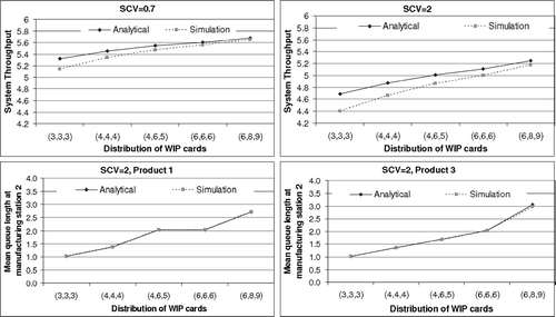
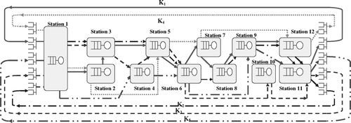
Fig. 6 Queuing network model for system in Experiment 2 with 12 machines and five products.

4.2. Experiment 2

This experiment investigates the performance of the parametric-decomposition-based approach on a larger network. In particular, a system with five products (R = 5) and 12 manufacturing stations (M = 12) is considered. Figure 6 shows the queuing model of the system considered in this experiment, and Table 2 indicates the product routing and service process parameters (μ _r,m and c ² _{s r,m} ) for each product at each station. The example is similar to Example 3 in Baynat and Dallery (1996), with modifications made in order to explicitly model demand and raw material arrivals for each product. Table 3 reports performance results corresponding to three different system configurations, namely:

	Case 1. λ P r,0 = 6, ∀ r; λ F 1,2 = 0.2, λ F 2,2 = 0.25, λ F 3,2 = 0.3, λ F 4,2 = 0.30, λ F 5,2 = 0.35, K 1 = 6, K 2 = 8, K 3 = 10, K 4 = 7, K 5 = 9.
	Case 2. λ P r,0 = 6, ∀ r; λ F 1,2 = 0.2, λ F 2,2 = 0.25, λ F 3,2 = 0.3, λ F 4,2 = 0.30, λ F 5,2 = 0.35, K 1 = 12, K 2 = 15, K 3 = 11, K 4 = 13, K 5 = 10.
	Case 3. λ P r,0 = 6, ∀ r; λ F 1,2 = 0.25, λ F 2,2 = 0.25, λ F 3,2 = 0.35, λ F 4,2 = 0.40, λ F 5,2 = 0.45, K 1 = 16, K 2 = 20, K 3 = 18, K 4 = 14, K 5 = 19.

Table 2 Routing and service process parameters for network in Experiment 2

	Machine service rates and SCV at each machine: (μ r,m , c ^2 sr,m )
	1	2	3	4	5	6	7	8	9	10	11	12
Product 1	(1,1)	(0.5, 1)	(1,1)		(1, 0.5)	(1.33, 8.5)	(2, 1)	(1, 1)	(0.8, 1)		(4, 1)	(1.33, 1)
Product 2	(2,1)		(1,1)		(1, 5)	(2.5, 2.5)		(1, 1)	(0.8, 1)		(0.5, 1)	(2, 1)
Product 3	(4,1)		(1,1)	(2, 1)	(2, 2.2)	(1.11, 2.1)				(0.67, 1)		(1, 1)
Product 4	(10,1)	(0.5, 1)			(0.5, 5)		(2, 1)				(1, 1)
Product 5	(1.33,1)			(2, 1)		(0.8, 5.8)			(0.8, 1)			(4, 1)

Table 3 Performance results for Experiment 2

	λ1	λ2	λ3	λ4	λ5
Case 1
A	0.123	0.164	0.227	0.214	0.304
S	0.117	0.180	0.253	0.238	0.322
E	5.119	−8.791	−10.313	−10.319	−5.624
Case 2
A	0.150	0.195	0.192	0.228	0.302
S	0.151	0.210	0.221	0.248	0.314
E	−0.912	−7.160	−13.397	−8.300	−4.104
Case 3
A	0.153	0.190	0.231	0.227	0.365
S	0.151	0.203	0.256	0.253	0.384
E	1.463	−6.392	−9.897	−10.200	−4.760
A: Analytical, S: Simulation, E: %Error.

In all three cases, c ² _{P r,0} = c ² _{F r,2} = 1, K _r,0 = 8, K _r,2 = 4, ∀ r. The results indicate that the throughput estimates for the larger network are within 10% of the simulation estimates for most cases. While the error in estimates appears to increase with network complexity, such trends are observed with other approaches discussed in the literature as well. The next experiment compares the performance of the parametric-decomposition-based approach with two different approaches reported in literature.

4.3. Experiment 3

This section compares the performance of the parametric-decomposition-based approach with the product-form approximation approach proposed by Baynat and Dallery (1996) (Experiment 3.1) and the approach proposed by Ryan and Choobineh (2003) (Experiment 3.2). In Experiment 3.1, a network with five products (R = 5) and 12 manufacturing stations (M = 12) is considered. The products have probabilistic routing and the network configuration is same as that considered in Example 3 in Baynat and Dallery (1996). Table 4 summarizes the results of the comparison. From this experiment, it appears that the error levels in the estimation of throughput using the parametric decomposition method are comparable to those obtained using the product-form approximation approach of Baynat and Dallery (1996) on the same network. Experiment 3.2 considers a network with two products (R = 2) and six manufacturing stations (M = 6). The network configuration is the same as that considered in Example 1 in Ryan et al. (2000). Table 5 summarizes the results of the comparison. From the comparison experiments it appears that the parametric-decomposition-based method yields marginally better estimates of throughput as compared to those reported in Ryan et al. (2000).

Table 4 Performance results for Experiment 3.1: comparison with Baynat and Dallery (Baynat and Dallery, 1966)

(K 1,K 2,K 3,K 4,K 5)		λ1	λ2	λ3	λ4	λ5
(6, 8, 10, 7, 9)	Baynat and Dallery	0.195	0.352	0.439	0.241	0.431
	This paper	0.182	0.329	0.411	0.211	0.422
	Simulation	0.182	0.327	0.433	0.237	0.410
(12, 15, 11, 13, 10)	Baynat and Dallery	0.237	0.460	0.364	0.240	0.403
	This paper	0.226	0.434	0.318	0.218	0.411
	Simulation	0.227	0.430	0.360	0.237	0.387
(16, 20, 18, 14, 19)	Baynat and Dallery	0.250	0.445	0.441	0.227	0.444
	This paper	0.243	0.425	0.391	0.205	0.467
	Simulation	0.243	0.423	0.434	0.226	0.431

Table 5 Performance results for Experiment 3.2: comparison with Ryan et al. (2000)

(K 1, K 2)		Network Throughput
(5, 10)	Ryan et al.	0.253
	This Paper	0.243
	Simulation	0.247
(7, 16)	Ryan et al.	0.261
	This Paper	0.253
	Simulation	0.255
(8,19)	Ryan et al.	0.263
	This Paper	0.256
	Simulation	0.258
(8,10)	Ryan et al.	0.277
	This Paper	0.269
	Simulation	0.271

5. Conclusions

This paper proposes a parametric-decomposition-based approach for performance evaluation of queuing network models of multi-product systems with CONWIP control. Two-moment approximations are first used to characterize the performance measures at fork/join stations and manufacturing stations in the network. Subsequently, stochastic transformation equations are used to link the traffic processes at the different stations in the network, and the resulting set of non-linear equations is solved using an iterative algorithm to obtain the performance measures of interest.

The approach presented has some qualitative advantages over previous approaches for analysis of closed queuing network models of multi-product CONWIP systems, such as Baynat and Dallery (1996) and Ryan and Choobineh (2003). In the product-form approximations used by Baynat and Dallery (1996) the number of unknown parameters (namely the load-dependent arrival and service rates at the different stations) grows with the network population. In contrast, in the parametric-decomposition-based approach, the number of unknown parameters (mean and variability parameters of the traffic processes) is independent of the network population. Ryan and Choobineh (2003) use a non-linear programming-based approach to analyze multi-product CONWIP systems. Their approach is tested for several systems operating under exponential service time assumptions and some sensitivity analysis is done using simulation to test the impact of other service time distributions. The approach proposed in this paper, provides a more elaborate model of variability. In particular, the approach explicitly models variability in the arrival processes of raw materials, demand and processing times at the manufacturing stations. Therefore, the effects of different types of variability on system performance can be directly studied.

In terms of numerical accuracy, the approach yields throughput and mean queue length estimates that are comparable to that of the product-form approximation approach in Baynat and Dallery (1996), and marginally better than than obtained using the approach reported in Ryan et al. (2000). Although a more exhaustive study of the different approaches is required to provide more conclusive comparison results, it does appear that the parametric decomposition approach provides an alternative method for performance evaluation that avoids the need to compute multiple load-dependent arrival and service rates, and yet provides performance estimates with comparable accuracy. Finally, the approach can be used to develop efficient decomposition-based approaches for multi-stage multi-product systems under pull-type controls with batch size and set up constraints. Parametric decomposition approaches based on two-moment approximations closely lend themselves to the analysis of such systems without significant increase in computational complexity (Vandaele et al., 2002; Satyam and Krishnamurthy, 2006). These extensions are currently being investigated.

Biographies

Kumar Satyam is a Ph.D. candidate in the Department of Decision Sciences and Engineering Systems at Rensselaer Polytechnic Institute (RPI), located in Troy, NY, USA. He holds a Master's degree (M.S.) in Industrial and Management Engineering from RPI, and a Bachelor's degree (B.Tech) in Industrial Engineering from the Indian Institute of Technology (IIT), Roorkee, India. His current research focuses on performance evaluation of multi-product systems operating under various forms of pull-control strategies. He is a member of INFORMS and IIE.

Ananth Krishnamurthy is an Assistant Professor in the Department of Decision Sciences and Engineering Systems at Rensselaer Polytechnic Institute (RPI), located in Troy, NY, USA. He obtained his Ph.D. from the University of Wisconsin-Madison in 2002. His research focuses on topics including production inventory control, assembly operations, material handling and warehouse systems, product variety, customization, lead time reduction and quick response manufacturing. He is a member of INFORMS, IIE, SME and APICS.

References

- Baynat , B. and Dallery , Y. 1996 . A product-form approximation method for general closed queuing networks with several classes of customers . Performance Evaluation , 24 : 165 – 188 .
- Bitran , G. R. and Tirupati , D. 1988 . Multiproduct queuing networks with deterministic routing: decomposition approach and the notion of interference . Management Science , 34 ( 1 ) : 75 – 100 .
- Bonvik , A. M. , Dallery , Y. and Gershwin , S. B. 2000 . Approximate analysis of production systems operated by a CONWIP/finite buffer hybrid control policy . International Journal of Production Research , 38 ( 13 ) : 2845 – 2869 .
- Broyden , C. G. 1965 . A class of methods for solving non-linear simultaneous equations . Mathematics of Computation , 19 : 577 – 593 .
- Buzacott , J. A. and Shantikumar , J. G. 1993 . Stochastic Models of Manufacturing Systems , Englewood Cliffs , NJ : Prentice Hall .
- Duenyas , I. 1994 . A simple release policy for networks of queues with controllable inputs . Operations Research , 42 : 1162 – 1171 .
- Hopp , W. and Roof , M. 1998 . Setting WIP levels with statistical throughput control (STC) in CONWIP production lines . International Journal of Production Research , 36 : 867 – 882 .
- Kamath , M. , Suri , R. and Sanders , J. L. 1988 . Analytical performance models for closed-loop flexible assembly systems . The International Journal of Flexible Manufacturing Systems , 1 ( 1 ) : 51 – 84 .
- Krishnamurthy , A. and Suri , R. 2006 . Performance analysis of single stage kanban controlled production systems using parametric decomposition . Queuing Systems: Theory and Applications , 54 : 141 – 162 .
- Krishnamurthy , A. , Suri , R. and Vernon , M. 2003 . “ Two-moment approximations for throughput and mean queue length of a fork/join station with general input processes ” . In Stochastic Modeling and Optimization of Manufacturing Systems and Supply Chains , Edited by: Shantikumar , J. G. , Yao , D. D. and Zijm , W. H.M. 87 – 126 . Kluwer .
- Ryan , S. M. , Baynat , B. and Choobineh , F. 2000 . Determining inventory levels in a CONWIP controlled job shop . IIE Transactions , 32 : 105 – 114 .
- Ryan , S. M. and Choobineh , F. 2003 . Total WIP and WIP mix for a CONWIP controlled job shop . IIE Transactions , 35 ( 3 ) : 405 – 418 .
- Ryan , S. M. and Vorasayan , J. 2005 . Allocating work in process in multi-product CONWIP system with lost sales . International Journal of Production Research , 43 : 223 – 246 .
- Satyam , K. and Krishnamurthy , A. Analytical models for multi-product pull systems with batch sizes . Presented at the Industrial Engineering Research Conference . Orlando , FL .
- Spearman , M. 1992 . Customer service in pull production systems . Operations Research , 40 : 948 – 958 .
- Spearman , M. , Woodruff , D. and Hopp , W. 1990 . CONWIP: A pull alternative to kanban . International Journal of Production Research , 28 : 879 – 894 .
- Spearman , M. and Zazanis , M. 1992 . Push and pull production systems: Issues and comparisons . Operations Research , 40 : 521 – 532 .
- Vandaele , N. , Boeck , L. D. and Callewier , D. 2002 . An open queuing network for lead time analysis . IIE Transactions , 34 : 1 – 9 .
- Whitt , W. 1983 . The queuing network analyzer . The Bell System Technical Journal , 62 ( 9 ) : 2779 – 2815 .
- Whitt , W. 1994 . Towards better multi-class parametric decomposition approximations for open queuing networks . Annals of Operations Research , 48 : 221 – 248 .