Clusters and filling-curve-based storage assignment in a circuit board assembly kitting area

Abstract

Kitting is the process that gathers all of the components necessary to assemble a batch of circuit boards on production machines. An objective in kitting storage design is to minimize the travel involved in collecting the components in the storage area so as to decrease labor costs. From outward appearances, the kitting process is similar to order picking in a warehouse. Closer observation, however, reveals that its unique characteristics favor a cluster-based allocation over the storage strategies usually adopted in warehouses. We present a clustering and cluster assignment method. In the clustering method we develop a new objective function and incorporate it into a genetic algorithm. In the cluster assignment method we first develop a new index for cluster assignment priorities. We then prove optimum assignments of clusters under restrictive conditions and extend the result to realistic storage configurations using filling curves. We analyze the properties affecting the quality of filling curves and develop a class of filling curves with good performance characteristics. Finally, we perform numerical analyses to show that the cluster and filling-curve-based assignment in the kitting area can reduce travel distances.

Keywords:

• Kitting
• order picking
• storage
• cluster
• filling
• curve
• cubic order index
• grouping
• circuit board

1. Introduction

The components used in circuit board assembly are generally stored in an area that is similar to a small warehouse. When the order to produce a batch of boards is released, the components required to assemble the boards need to be gathered from their storage locations and delivered to the production line. This process is called kitting, and the area where it is performed is called the kitting area. Hundreds of different board types tend to be assembled at individual assembly plants. Each individual board design may contain hundreds of different components. Therefore, a plant usually needs to store thousands of different components, often in reels. Going to various locations to pick these components involves a considerable amount of travel and incurs labor cost. If the batch size is small, the kitting time can be longer than the time spent on the production machines and can be a bottleneck to efficient operation of the expensive assembly line.

The travel time is determined by the travel distance, which in turn is determined by the storage location assignment (or allocation) and picking route. Our objective in this research is to minimize the long-term average travel distance by optimizing the storage allocations. The problem can be considered to be a Storage Location Assignment Problem (SLAP). The major objective of location assignment is to reduce the travel distance. The SLAP is known to be NP-complete. The decision variables in this study include the combination of two sets of factors: component allocations and the picking tours. The size of the former is in the hundreds to thousands whereas the size of the later is NP-hard by itself.

A kitting area is similar to a warehouse in that a picker goes around the storage area following a pick sheet. However, closer observations reveal that the kitting area has several unique features not normally found in a warehouse.

1.	In kitting, the pick sheet is the Bill of Materials (BOM) as opposed to customer orders in a warehouse. BOMs are based on the product designs, which are relatively stable compared to customer orders.
2.	BOMs contain components for certain functional blocks. Therefore, the correlations among BOMs are higher and deterministic compared to customer orders in a warehouse.
3.	BOMs usually contain tens to hundreds of line items in the form of a Stock Keeping Unit (SKU). However, the number of line items of customer orders in warehouses varies from a few to many.
4.	The cost of many electronic components is high but the size of a component is small. As a result, a reel can hold all the components of one SKU available in a plant. It is not desirable to keep them in both fast pick and reserve locations.
5.	A picker can carry many reels in one trip in the kitting area. However, the sizes of items vary a lot in warehouses, and a picker often can pick only one case per trip.

To reduce travel distances, warehouses adopt fast pick, batch picking and zone picking with a common pick area strategies. The use of a fast pick approach requires storage in both the pick and reserve areas, which is often not desirable in kitting because of feature 4 above. In addition, it is not likely that all SKUs in a BOM will be in the fast pick area. A large amount of travel for a few SKUs in the scattered reserve area would negate any savings created by the fast pick approach. Batch picking consists in picking a batch of orders in a single trip. It is often beneficial when the pick list is short. Nonetheless, feature 3 indicates that BOMs often contain a long list of SKUs. Zone picking uses staffed picking zones to share the task of order picking. It reduces the travel distances for pickers in zones and achieves a shorter pick cycle. However, if the volume is low, the utilization of dedicated pickers in the zones can be low. If the volume is high, our proposed clustering approach would further speed up picking in the zones. The use of a common pick area will not significantly reduce the travel distance if natural clusters exist because a picker has to visit the clusters for other SKUs.

These characteristics in the kitting area suggest that a good strategy to reduce the travel distance is to place the SKUs of a BOM into a single or just a few clusters. A picker can travel to the cluster(s) and pick multiple components with little travel inside a cluster. Ideally, we would like to find SKU–BOM clusters such that each cluster of SKUs contains exactly all the components required by one type of circuit boards. Further travel reduction is possible by allocating clusters to more convenient locations based on the pick frequency and space requirements.

Based on the aforementioned rationale, we develop a cluster and cluster allocation method for SLAPs. This paper addresses the theoretical aspects of the method and presents a preliminary numerical study. It is structured as follows. We develop a new objective function able to cluster BOMs and SKUs that is incorporated into an existing genetic algorithm. For cluster allocation, we first develop a new Cube-per-Order Index (COI) for the prioritization of clusters. We first find the optimum allocation in a one-dimensional space. Then we apply the concept of filling curves to expand the results to two-dimensional space to find the optimum solution under certain conditions. We discuss the characteristics of filling curves and their importance to our application and present some effective filling curves. We then study the effect of correlations between the clusters and develop the adjusted COI and objective function. Finally, we perform numerical analyses to show that the cluster and filling-curve-based storage in the kitting area can reduce travel distances.

We will present the literature related to clustering and optimum location assignment problems in the corresponding sections.

2. Cluster analysis

2.1. BOM/SKU incident matrix

Cluster analysis consists in findings clusters in the BOM/SKU incidence matrix F, defined as follows. Let:

	j ∈ {1, …, J} be the index for SKU j , i.e., a component type in the board assembly;
	i ∈ {1, …, I} be the index for BOM i , i.e., the list of components of a board design i;

F be a BOM/SKU incidence matrix where

Assume that after the clustering process, N clusters are generated along the diagonal of the matrix F, labeled as h ₁, h ₂, …, h _N . We use S _{h n} and B _{h n} to represent the corresponding sets of SKUs and BOMs of cluster h _n . Define a set of cluster matrices H = {H ₁, H ₂, … H _n , …, H _n } where H _n is the nth diagonal block in the BOM/SKU matrix F. We will use H _n (i, j) to represent the corresponding elements in H _n . H _n (i, j) = 1 if the corresponding BOM i contains SKU j. H _n is a matrix of size(B _{h n} ) × size(S _{h n} ). We define the correlation matrix between cluster matrices H _m and H _n by Corr _m,n :

where i ∈ B _{h m} , j ∈ S _{h n} . We will use Corr _m,n (i, j) to represent elements in Corr _m,n . Corr _m,n (i, j) = 1 if the BOM i belongs to cluster h _m , SKU j belongs to cluster h _n , and BOM i contains SKU j. These definitions are shown in Equation (1).

In general, Corr _m,n ≠ Corr _n,m

Analysis of clustering behavior has been reproted in the literature using various methods. Rather than focusing on the clustering process itself, we focus on producing an objective function that is suitable for kitting.

2.2. Clustering objective: Weighted grouping efficiency

The ideal clustering result is an incidence matrix in which all entries are in the diagonal blocks with no gaps being present in these blocks. However, the ideal result may not exist, or it may be intractable, meaning that a solution can not be found in a reasonable amount of time for practical problems. When there are entries outside the diagonal blocks, the picker has to travel outside of the clusters. When there are gaps within the diagonal blocks, the picker has to travel more within the clusters. A good objective should penalize both entries outside of the cluster and gaps inside the cluster with an appropriate weight. One may surmise that entries outside of a cluster can lead to more travel than gaps inside the cluster.

Chandrasekharan and Rajapopalan (1986) introduced the grouping efficiency η. It is the weighted sum of the fraction of entries in the clusters and the number of voids outside the clusters. Kumar and Chandrasekharan (1990) found that the entries and voids are not balanced when the number of blocks becomes large. They suggested a grouping efficacy Γ that represents an improvement. However, it does not consider the build frequency of a BOM or provide a weight to trade-off between undesirable entries and voids. Adding the build frequency, weight for entries outside of the diagonal and gaps in the cluster, and normalizing the measure, we arrive at a new cluster objective function, the weighted grouping efficiency:

where

e	=	∑ A i × b i is the sum of frequency-weighted entries in the diagonal blocks;
e v	=	∑ A i × v i is the sum of frequency-weighted gaps in the diagonal blocks;
e 0	=	∑ A i × (s i − 1) is the sum of frequency-weighted entries outside of the diagonal blocks;
A i	=	build frequency of BOM i;
b i	=	number of entries in the diagonal blocks in row i;
v i	=	number of gaps in the diagonal blocks in row i;
s i	=	number of clusters that BOM i encounters;
β	=	weight between zero and one to weigh the effect of e v and e 0.

This objective incorporates build frequencies and a weight β, where 0 ≤ β ≤ 1. If one wants to weight the entries outside the clusters more, one can increase β and vice versa. Note that 0 < Γ ≤ 1, and Γ = 1 if and only if e _v = e ₀ = 0 (or perfect clustering).

2.3. Cluster formation

We adopt the genetic algorithm proposed by Joines et al. (1996) to form the clusters due to its ability to accommodate different objective functions. In our case, the objective function is the grouping efficiency Γ. We define two sets of variables for chromosome representation: x _i ∈ {1, …, N}, i ∈ {1, 2, …, I} and y _j ∈ {1, …, N}, j ∈ {1, 2, …, J}. If x _i = m, BOM i is assigned to cluster m; if y _j = m, SKU j is assigned to cluster m.

We define individual to be a vector of I + J integers with values from one to N, where N represents an upper bound on the number of clusters to be formed:

We chose N before starting the execution. The larger the value of N, the larger the search space, but if the chosen N is too large, the algorithm will generate empty clusters, i.e., clusters that contain neither SKU nor BOM.

We randomly generate a set of individuals as the initial population. Each individual will correspond to a different BOM/SKU matrix, and we evaluate each individual's grouping efficiency Γ. The individual with the highest grouping efficiency Γ is assigned a higher probability of being a parent in all successive generations.

Mutation and crossover operations are used to search for a higher grouping efficiency Γ from generation to generation. In mutation, only one individual is picked to be a parent. Starting from this individual, we randomly pick an SKU or BOM and move it to another cluster. This is equivalent to changing the position of the corresponding column or row in the BOM/SKU matrix. In the chromosome representation, this is equivalent to assigning a random element of the individual to another valid value. In the crossover operation we pick two individuals from the population to be parents. We name them parent 1 and parent 2. Then, a splice point will be chosen randomly. Both parents are cut at the splice point. The front portions of each parent are combined with the end portion of the other parent. To keep the candidate pool at a stable size, we replace some parents with their children after each generation if a higher grouping efficiency Γ is discovered. We terminate the genetic algorithm when the maximum generation limit is met.

3. Allocation of perfect clusters

Results are available for optimum single-command cycle location assignments in the literature, but clustered storage does not fit into single-command cycles. We first assume that the created clusters are perfect—that is there are no gaps in the clusters and no correlations between clusters exist. In reality, the clusters are normally imperfect; we will discuss the effect of gaps and correlations in Section 5. We assume that a picking tour starts from an Input/Output (I/O) location, travels to the near end of the cluster, passes each location in the cluster, reaches the far end of the cluster, and returns to the I/O location. We assume the travels form a path with the shortest distance along the aisles. We first define a suitable COI for clusters and find an optimal location assignment in one-dimensional space. We then extend the result to two-dimensional space with various filling curves, find the optimum solution for this two-dimensional space under certain conditions and develop quantitative metrics to show the degree of deviation from optimum conditions.

3.1. Location assignment in one-dimensional space

Consider a simple one-dimensional rack that has one layer and an unlimited length. The I/O point is located at one of its ends. Starting from this end, the rack is divided into equal slots of unit length d, labeled l, shown in Fig. 1. The travel distance from the I/O point to the lth slot equals l unit lengths.

Fig. 1 One-dimensional rack.

The problem is to find the optimum sequence among the N! possible sequences that minimize the total travel distance. For single-item storage and a single-command cycle, an O(NlogN) algorithm based on the concept of a COI was introduced by Heskett (1964). The index for an item is defined as the ratio of its space requirement and order frequency. In his solution, SKUs are sorted by the COI in ascending order and allocated to storage locations in non-decreasing order of distance from the I/O point. Francis and White (1974) and Harmatuck (1976) later proved that this method is optimal for single-command cycles. However, when picking is not performed under a single-command cycle, as is the case for cluster storage, the optimality no longer holds.

Frazelle (1990) and Lee (1992) applied the COI concept to clusters. They defined the COI for clusters as the ratio of the total space requirement of a cluster and the sum of the build frequencies of all SKUs in the cluster. This definition captures the visit frequencies to the individual locations in a cluster. However, in cluster-based storage, the travel affected by cluster assignment is between the I/O point and the clusters. The frequency of visiting a cluster is that of the BOMs supported by the cluster. This frequency is lower than the sum of frequencies of all individual SKUs in the cluster. Therefore, we define COI _n for cluster n as the ratio of the total space requirement of a cluster and the sum of the build frequencies of the BOMs in the cluster:

where C _j is the number of locations required to store SKU j.

Later, we will prove that the optimum assignment of perfect clusters in the one-dimensional space is in increasing order of COI _n values. This provides an efficient algorithm with complexityO(NlogN).

3.2. Mapping two-dimensional spaces using filling curves

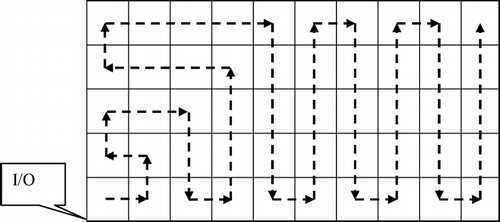
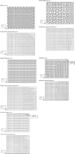
In reality, kitting areas are two-dimensional or three-dimensional and have different shapes and sizes. Using the concept of a filling curve, we can map a general space into a one-dimensional rack. A filling curve is a continuous mapping from a one-dimensional space into a higher-dimensional space. In our application, any curve going through each location of the kitting area is a potential filling curve. For example, a curve connecting non-decreasing Chebychev distance locations (applicable in automatic storage/automatic retrival systems with an I/O point at the lower-left corner) is a filling curve, as shown in Fig. 2. Following the sequence along this filling curve, locations in a two-dimensional picking face can be mapped into a one-dimensional rack. We will label the cells along the curve as l ∈ {1, …, L}, where L is the last location on the curve.

Fig. 2 A feasible filling curve of a square-in-time automatic storage and retrieval system.

A special type of filling curve is the space-filling curve. Nulty (1993) noted that some space-filling curves have excellent clustering properties. Bartholdi and Goldsman (2001) showed that the use of space-filling curves can lead to the creation of a simple heuristic to solve the Traveling Salesman Problem (TSP). Another feature of a space-filling curve is the interchangeability of blocks along the curve. Bozer et al. (1994) and Meller and Bozer (1996) used this feature and the clustering property of space-filling curves to solve facility layout problems when interdepartmental material flow is of concern.

3.3. Location assignment along filling curves

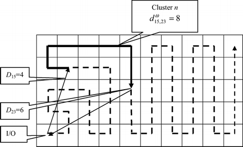
Let Ω = {1, …, ω, …} be a set of filling curves, ω (1), ω (2), …, ω (l)…, ω (L) be the locations along the filling curve ω, d _lk ^ω be the distance between location l and location k along the filling curve ω, and D _l be the shortest distance from the I/O point to location l. The shortest distance can be Euclidean, rectilinear or another metric that is suitable for the problem. In warehouses with perpendicular aisles, a suitable metric is the rectilinear distance.

For convenience, let the space requirements for cluster n be

and the cluster build frequency

If we store clusters h ₁, …, h _n , …, h _N sequentially along the filling curve ω, then the location of the first SKU for the nth cluster is after location R _n = ∑ _{k = 1} ^{n − 1} r _k and the total travel distance is

where the first term in the parentheses is the distance from the I/O point to the first item in cluster n, the second term is the travel distance within cluster n along the curve, and the last term is the travel distance from the last SKU in cluster n back to the I/O point as shown in Fig. 3.

Fig. 3 Picking route of a cluster stored along a filling curve.

For a one-dimensional rack with a pick face of one unit in width, one can verify that Equation (4) becomes:

In two dimensions, a lower bound of the shortest total travel distance can be obtained as follows. Sort locations in the kitting area in increasing order by their rectilinear distance to the I/O point, represented by D ₍₁₎, D ₍₂₎, …, D _(L). Sort the picking frequency of each cluster in decreasing order, represented by f ₍₁₎, f ₍₂₎, …, f _(N). The number of locations occupied by these clusters are r ₍₁₎, r ₍₂₎, …, r _(N). We can find a lower bound by using the lowest possible distances for all three terms in Equation (4):

where d is the distance between adjacent locations. Adjacent locations share a common edge, as in a one-dimensional rack.

3.4. Properties of filling curves and their metric

Racks in higher-dimensional spaces along the filling curves in realistic warehouses differ significantly from the simple one-dimensional rack. There are turns, aisles and obstacles. We now discuss three factors that provide quantitative measures of deviation from the one-dimensional rack.

3.4.1. Curve length factor μ

In the simple one-dimensional rack, the distance between adjacent locations is a constant. However, the travel between adjacent locations along a filling curve at turns, across aisles, and around the end can be different. Let the shortest distance between any pair of locations (l, l + 1) be d _min(l, l + 1). One desirable factor for a curve to stay close to optimality in two dimensions is to have minimum extra distances. We define the curve length factor as the ratio of the total length of a filling curve to the minimum length:

In practical situations, d _min(l, l + 1) is equal to or greater than the minimum distance in a one-dimensional rack, d. Then, μ _ω ≥ 1, and μ _ω = 1 if and only if all the distances between nearby locations along curve ω are equal to the minimum linear distance between adjacent locations. The value of μ _ω depends not only on the filling curve but also on the physical configuration of the kitting area. Most kitting areas have multiple racks. When a picker goes from back-to-back locations, that picker should go around the end (as in being at the end of library shelves). A picker may also need to travel across the aisle between two racks. The width of the aisle is normally greater than the distance between nearby locations within the same rack.

3.4.2. Gap variation factor σ

Unlike a one-dimensional rack, the distances between consecutive locations along the curve in a two-dimensional rack change at turns and at the end of aisles. If large gaps occur in the middle of a cluster, the total travel distance may increase. Large gaps can also be found with hallways or columns. The gap variation can be captured by the coefficient of variation for random variables:

where avg(d _{n,n + 1} ^ω) is the average distance between adjacent locations along the curve and avg((d _{n,n + 1} ^ω)²) is the average of the square of the distances. The expression inside the square root of the numerator is the evaluation using variance for random variables although the distances are deterministic with a given design. Here, σ _ω ≥ 0, with σ _ω = 0 if all distances between nearby locations along the filling curve are the same.

3.4.3. Distance proportionality property λ

In a simple one-dimensional rack, the distance from the I/O point to a location l is proportional to index l. The proportionality is required for optimality using COI-based allocation for multi-command cycles. However, in higher-dimensional spaces, the minimum distance from the I/O point to a location l along a curve is most likely not proportional to the index on the filling curve.

Theorem 1. If μ_ω = 1 and the shortest distance from the I/O point to each location is proportional to its index in the filling curve, the cluster with the lower COI should be stored closer to the I/O point along this filling curve in the optimal sequence.

Proof. A proof is given in Appendix A.

Since the one-dimensional rack is a special case of Theorem 1, the assignment of clusters in increasing order of COI for a one-dimensional rack is optimum. In many cases, however, a filling curve satisfying the conditions of Theorem 1 cannot be found. However, we can use the departure from proportionality condition to measure a curve. We define the distance proportionality factor as the average difference from the proportional distance:

where g is a constant. In one-dimensional racks, g = 1. In two-dimensional spaces, g is usually less than unity because the shortest distance between two points is a straight line and not a curve. If the distance to the I/O point along a curve is proportional to the index of the locations, the total distance from the I/O point to every location will be

which is equal to ∑ _{l = 1} ^L D _l . Thus,

Equation (9) shows that the value of g is a function of the shape of the area but not of the filling curves. We call g the geometric constant.

One can verify that the proportional distance factor λ _ω ≥ 0 with λ _ω = 0 if and only if the distance from the I/O point to each location along the filling curve is proportional to its index in the filling curve.

These three factors, μ _ω, σ _ω and λ _ω, affect the quality of using the COI method along filling curves. If a curve satisfies the conditions μ _ω = 1, σ_ω = 0 and λ _ω = 0, an increasing COI will provide the optimal sequence of cluster assignments along the curve. Any violation of the above conditions will lead to less confidence in the optimality.

3.5. Multiple filling curves

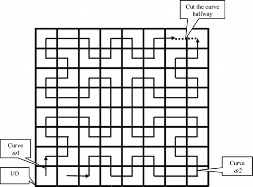
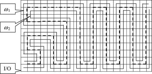
One way to improve the filling curve quality with racks is by using multiple filling curves. For example, we can divide Moore's version of the Hilbert space-filling curve (Sagan, 1994) from corner to corner, shown in Fig. 4. Before division, the three properties of the single curve are:

After division into two half curves (the two curves start and end at different locations), the properties are:

Fig. 4 Two filling curves in an 8 × 8 square space.

Whereas the length and gap factors remain constant, the average proportionality factors have been reduced by about 60% for both half curves.

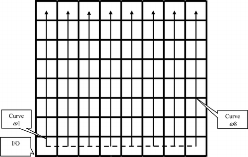
A special type of multiple filling curve is a set of parallel finite-length one-dimensional racks linked at one end as shown by the dashed lines shown in Fig. 5. All three factors for this curve will be ideal. This multiple curve is especially suitable to pick along the aisles.

Fig. 5 Multiple filling curves in an 8 × 8 square space.

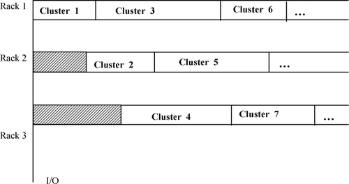
When a group of V infinite-length parallel one-dimensional filling curves is used in a zoning process, the structure will be similar to V independent one-dimensional racks as in Fig. 6. The different racks are independent of one another except that they are connected to the same I/O point with different offsets, which are modeled by the shaded areas. Assume that the clustering process generates N perfect clusters. The problem is how to assign and sequence the N uncorrelated clusters in the V one-dimensional racks.

Fig. 6 Multiple one-dimensional racks.

Theorem 2. If all clusters are of the same build frequency, the optimal zoning can be obtained in polynomial time.

Proof. See Appendix A.

Theorem 3. If all clusters are of the same size, the optimal sequence can be found in polynomial time.

Proof. See Appendix A.

The condition in Theorem 3 is a practical one. The kitting area manager may want to assign zones of equal size to every cluster to simplify operations. If a zone can hold more SKUs than a cluster requires, some locations in the zone may remain empty. If other clusters are assigned beyond this zone, there is “waste” of closer spaces. However, the extra capacity can be helpful if BOMs change later. If the zones assigned to all clusters are equal, the COI is equivalent to the index of the build frequency.

In the above discussion, we did not consider a finite rack length. This constraint may not be binding if the available locations are more than those required by all the SKUs. If no clusters have to be split at the end of the aisle, the constraint is not binding. Even when the constraint is binding, only the less visited clusters with a higher COI are affected. Normally, aisles connect the ends of racks; therefore, splitting a cluster into adjacent racks at the end of an aisle may not cause excessive travel. In other words, the extra travel due to a finite rack length should not be excessive in practice.

3.6. Concept of a dual filling curve

Observe that in the simple one-dimensional rack, after visiting the last SKU at the end of a cluster, a picker will revisit all the SKUs in the same cluster on his or her return to the I/O point. This means that the picker will visit the same location twice in the one-dimensional rack structure. This travel distance can be reduced if SKUs in a cluster are arranged in a “U” shape. Consider a kitting area of two parallel one-dimensional racks. If COI-based allocation is applied, the zoning result is shown in Fig. 7. The distance from the starting position of cluster n to the I/O point is

Fig. 7 Zoning in two one-dimensional racks.

If the number of locations occupied by each cluster is uniformly distributed, the expected starting position of cluster n is

where _n is the average number of locations occupied by each cluster. The expected total travel distance is

If the two racks are close to one another, we can store half of the SKUs in each cluster on one rack and the other half on the opposite rack. In this case, the picker can pick part of each BOM while traveling along one rack and finish the BOM on the way back, as shown in Fig. 8.

Fig. 8 Zoning along two parallel one-dimensional racks.

The expected starting position and ending position of cluster n are (n − 1) _n /2, the expected total travel distance is ∑ ^N _{k = 1} ^N f _n n _n , and the savings are

We call two parallel curves with U-shaped cluster storage in two-dimensions a dual filling curve. The dual filling curve is a mapping from two-dimensional space into two parallel continuous curves. A pair of dual filling curves ω ₁ and ω ₂ in a 2p × 2q rectangular space can be generated from a filling curve ω in a p× q space. Each location in the p × q space can be mapped into a two-by-two square block in the 2p × 2q space. The mapping from the square-in-time filling curve shown in Fig. 2 yields the pair of dual filling curves shown in Fig. 9.

Fig. 9 The dual filling curves of the 2p × 2q space.

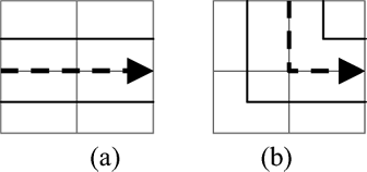
In the p × q space, the filling curve ω passes each location either in a straight line or with a 90° turn (called the straight-and-turn configuration). In the 2p × 2q space, the dual filling curves ω ₁ and ω ₂ pass each 2 × 2 block as shown in Fig. 10(a) and Fig. 10(b). In a straight path, both curves in the dual filling curve pass two locations. In turn, one curve passes three locations while the other curve only passes one. As a result, when we separate a cluster into two groups and assign each group along one curve respectively, the two groups may not occupy the exact same number of locations. However, if μ _ω = 1, then μ _{ω 1} = μ _{ω 2} = 1. By adjusting the SKUs into two groups, the total travel distance within each cluster will not be more than (r _n + 1) times the direct distance between adjacent locations. The distance between the ending location and the starting location will be less than twice that of the direct distance between the locations.

Fig. 10 (a) A straight path; and (b) a straight-and-turn configuration.

If the length or width of the kitting area is an odd number, one row or one column of the location cannot be covered by the dual filling curves. In that case, we can map the remaining locations using a single filling curve and store any remaining clusters along this curve. An example can be found in the numerical study.

4. The effect of correlation and procedures to handle its effects

In reality, perfect clusters may not be found. Correlations can affect both the COI-based cluster allocation and the performance of the resulting storage policies. We develop two methods to handle the correlations: adjustment of the COI definition and use of a common pick area.

4.1. The adjustment of the COI based on correlations

The COI method used in the allocation process depends on two factors of each cluster n: the build frequency f _n and the required space r _n . If correlations exist, f _n should equal the sum of the picking frequency of all BOMs encountering SKU cluster h _n . The set of these BOMs can be represented by

Note that B _{h n} ′ ⊇ B _{h n} since it includes BOMs other than B _{h n} . In other words, a cluster of SKUs will be visited more frequently because of the correlation. Therefore, the COI of cluster h _n needs to be adjusted as follows:

This definition is also valid for multiple filling curves and dual filling curves.

4.2. Common pick areas

Certain SKUs, such as power components, are so popular that they are included in almost every BOM. As a result, their SKU columns in the BOM/SKU matrix F have a lot of entries. After cluster analysis, these entries remain outside the diagonal blocks. One approach is to store them in the most convenient locations, such as adjacent to the production machines. By doing so, the decrease in correlation between clusters can be significant. However, the available convenient locations have a limited amount of space. We will refer to them as the common pick area.

We can construct the common pick area during the cluster analysis. We need to define a special cluster with limited capacity, for example, cluster 0. An SKU may be assigned to either a regular cluster or cluster 0. We will need one additional constraint:∑ ^J _{j = 1} ^J C _j y _j0 ≤ U, where y _j0 is a binary variable:

We also need to revise the grouping efficiency Γ by modifying the definition of e ₀ to e ₀′ = ∑ A _i (s _i ′ − 1) where s _i ′ equals the number of clusters that BOM i encounters other than cluster 0.

We can also construct the common pick area after the cluster analysis. Because the area is limited in size, the problem can be modeled as a knapsack problem. The capacity of the knapsack is U and the weight of SKU j is C _j . If SKU j is assigned to cluster n and moved into the knapsack, we shorten the trips of all BOMs that contain SKU j but do not belong to cluster n. The value of this move is

With these knapsack problem parameters, we can find the SKUs for the common pick area after cluster analysis.

5. Numerical study

We use both computer-generated data and industrial data to evaluate the benefit of the various aspects of clustering and the cluster allocation method. First, we study the effect of the number of clusters that BOMs visit. We derive an approximation method based on a theoretical estimate to compare the random storage of items to the random storage of clusters. Second, we study the COI-based allocation method to allocate perfect clusters to different filling curves. Third, we test the effect of weights in weighted grouping efficiency on an industrial data set. Last, we study the effect of a common pick area on the industrial data set.

5.1. The effect of the number of clusters

Daganzo (1984) showed that under rectilinear metrics and random storage, the estimated travel distance along the optimum TSP path is approximately E(TSP) ≈ G√AL, where G = 1.15 for rectilinear metrics, L is the number of uniformly distributed locations to be visited and A is the area. When correlations exist between clusters, a picker needs to visit other clusters. Daganzo's estimate can be modified to estimate the average total travel distance for the extra randomly located clusters.

Consider the case when the cluster analysis assigns BOM i with B _i SKUs to cluster n, and it is allocated along a filling curve ω with μ_ω = 1. In addition to SKU cluster n, BOM _i also encounters m _i other SKUs, which are uniformly distributed in the kitting area. Thus, the total travel distance for this BOM can be estimated as

where d is the distance between two adjacent locations. Here, we assume that the picker visits each SKU in its corresponding cluster, or m _i + 1 clusters in addition to the I/O point. For a specific BOM, this does not have to be the optimal route. Thus, Equation (13) is a suboptimal estimation of the travel distance of the cluster-based storage policy. The savings of the cluster-based storage policy over a random storage policy are

If the area of the aisle is neglected and each location is square, the area of the kitting area will be A = Ld ². The savings will be

The cluster-based storage policy will outperform the random storage policy if

Equation (16) can be used to estimate the cluster analysis effect without having information on the kitting area's physical configuration.

Consider a 15 × 20 storage area. Each slot is a 1 × 1 square block. We create 100 active BOMs. The picking frequencies range from one to 30 and are uniformly distributed. We arbitrarily assign the 100 BOMs to 20 clusters. The number of SKUs in each cluster ranges from ten to 19, respectively, and is uniformly distributed. We generate data sets using different seeds. We pick the data set that contains just under 300 SKUs or the capacity of the storage area. The number of SKUs in the first four sets that satisfy our condition are 289, 295, 285 and 280. The details of the data sets are given in Appendix B. We assume the picker travels in perpendicular aisles; therefore, rectilinear metrics apply. For the first data set, the total travel distance for random storage and the lower bound are

The average number of extra clusters visited, expected travel distances (using Equation (13), and the relative reduction from random storage are listed in Table 1.

Table 1 Estimated travel distance as a function of the number of extra clusters visited (m)

	Average m
	0	1	2	3	4	5	6	7
E(T)	65 283	75 241	83 636	91 033	97 720	103 869	109 593	114 968
Percentage reduction	46.5	38.3	31.5	25.4	19.9	14.9	10.2	5.8

5.2. Effect of filling curves on the application of COI-based allocation

We apply COI-based cluster allocation to five filling curves assuming perfect clusters are achieved. The curve descriptions, length factor, gap variation factor and proportionality factor are listed in Table 2. The two values of λ _ω for ω ₃ are for two curves. Every σ _ω is zero because we do not consider obstructions or gaps in the area. The geometries, distances and cluster allocations are listed in Appendix C.

Table 2 Curve parameters and travel distance using different filling curves

	Description	μω	σω	λω
ω 2	Non-decreasing rectilinear distance	1.89	0	2.30
ω 3	Variant of Moore's Hilbert space-filling curve	1	0	3.02/4.63
ω 4	Multiple filling curves	1	0	0
ω 5	Dual filling curve	1	0	1.75
ω 6	Multiple dual filling curves	1	0	0

The average distances traveled, the percentage improvements and the averages among all four data sets are summarized in Table 3.

Table 3 Estimated travel distance of different data sets

Curve	ω2	ω3	ω4	ω5	ω6	Random	Lower
Data set 1	80 321	64 314	64 775	57 775	55 324	122 044	36 129
Data set 2	116 783	91 324	94 599	88 455	79 337	174 938	52 275
Data set 3	66 569	54 053	53 991	50 146	44 845	105 163	31 913
Data set 4	104 638	85 337	86 357	79 412	71 988	163 775	50 854
Average percentage improvement	35	48	47	51	56

The average percent improvement among the four data sets over the random storage policy is significant and consistent.

5.3. Effect of weight β on the clustering objective

Our contention is that the entries outside of clusters lead to a larger distance increase than that of gaps in the clusters. To get some concrete quantitative evidence, we conduct cluster analysis using a weighted grouping efficiency with different weight values of β and then randomly allocate the clusters on multiple dual filling curves extended from ω ₅. We do not apply the COI-based allocation algorithm to see the isolated effect of β, which leads to conservative benefit estimates. To be more realistic, we use data from a medium-sized circuit board assembly original equipment manufacturer in a mid-volume, mid-mix manufacturing environment. The kitting area has 44 × 44 storage locations. The picker enters and departs the kitting area via a single entry at the corner. In a 3-month period, the 90 BOMs contain 1,759 SKUs. In this case, we conduct cluster analysis on the 90 × 1759 BOM/SKU matrix with different β values. The objective functions, average extra clusters visited and percentage improvement over random storage are listed in Table 4.

Table 4 Clustering result using different β values

	β
	0.5	0.6	0.7	0.8	0.9
Γ*	0.68	0.69	0.72	0.74	0.76
Average m	7.94	7.62	7.65	7.64	7.15
Percentage improvement	29.5	30.5	31.0	31.4	27.6

The improvement is about 30% when β is between 0.5 and 0.9, and the β * seems to fall between 0.7 and 0.9. It is consistent with our hypothesis that the correlation between clusters affects the travel distance more significantly than does additional walking within a cluster.

5.4. Effect of a common pick area

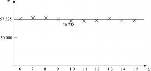
Finally, we investigate whether a common pick area can further improve performance using the industrial data. We consider the common pick areas to be at the lower-left corner with an area of U. We choose the cluster result of β = 0.8. The SKUs are assigned to the common pick areas based on the most clusters encountered.

We assume that the SKUs are in the common pick area and the clusters are uniformly distributed. The picker will visit the SKUs of the common pick area and then the other SKUs outside the common pick area. Among the SKUs of BOM i, p _i of them are selected for the common pick area. BOM i encounters m _i ′ additional clusters. The expected travel distance for picking this BOM is

Compared with the case with no common pick area, the travel distances with the common area at different sizes of U are shown in Fig. 11. The horizontal line represents the travel distance when there is no common pick area. Each × represents the travel distances at the corresponding size of the common pick area. The total travel reaches its minimum value at U = 10.

Fig. 11 Savings obtained using a common pick area with different sizes.

Compared to the no common pick area situation, the difference in travel is very small. The lack of change is not a surprise, as we argued in the Introduction.

5.5. Numerical study summary

From the numerical study, we see that the cluster and filling-curve-based storage assignment can significantly reduce travel distances. Without COI-based allocation on filling curves, the savings can be more than 40%. When COI-based clustering is used on multiple dual filling curves, the savings can be more than 50%. The savings with clustering alone, without the cluster allocation method, on a large industrial data set equaled 31%. We believe that β * should be greater than 0.5 because our results indicate that the travel between clusters affects the total travel distance more significantly than that of gaps in the clusters. A common pick area is not effective in kitting applications.

6. Conclusions

In this research, we developed a cluster and filling-curve-based storage method for the kitting area in circuit board assembly operations. We discovered the unique characteristics of the kitting area, and we developed a more suitable cluster objective and COI for clusters. We identified the various theoretical aspects of the COI-based location assignment on filling curves. Our numerical analysis shows that the filling curve is a simple yet effective method to assign the clusters of SKUs. The method can reduce travel distances significantly in comparison with a random storage policy if natural clusters exist.

Appendices

Appendix A: Proof of theorems

Proof of Theorem 1. With given conditions, D _l = g (l − 1), where g is a constant.

The total travel distance of the nth cluster along the filling curve will be

Assume that there is one optimal sequence, in which h _n is stored just in front of cluster h _{n + 1} along the filling curve, and COI _n ≥ COI _{n + 1}. The total travel distance for picking h _n and h _{n + 1} is

Switch h _n and h _{n + 1}, so that h _{n + 1} is stored in front of h _n along the filling curve. The total travel distance for picking h _n and h _{n + 1} will become:

while the travel distances for the other clusters are not affected.

The saving in total travel distance is Equation (A2) minus Equation (A3):

This is in contradiction with the optimality of the original sequence.

In a one-dimensional rack, adjacent clusters can be switched without influencing other clusters. However, in higher-dimensional spaces, the two clusters may require different storage spaces, and the switch may not be possible or it may affect other locations. In a one-dimensional rack, the return distance is equal to the one-way travel distance. Thus, the total travel distance should be doubled for both Equations (A2) and (A3). However, this does not affect the proof.

Proof of Theorem 2. Without loss of generality, assume that all build frequencies are equal to unity. We will map the cluster assignment problem into a non-preemptive parallel machine scheduling problem. V parallel racks can be mapped into V parallel machines represented in a Gantt chart. The length of clusters can be mapped to processing time on machines. The objective of minimizing the total travel is then equivalent to minimizing the total flow times of all jobs. Bruno et al. (1974) showed that polynomial-time solution can be obtained by a bipartite matching process for this problem. The details are as follows.

Using an idea stated in Bruno et al. (1974) we state that if a cluster that requires r locations is assigned as the last cluster on a rack than it will contribute r to the total travel distance. Similarly, if it is next to last, it contributes 2r and so forth, contributing kr if assigned as the kth cluster from the last. If this rack is offset by distance x _v from the I/O point there will be an additional travel distance x _v . The total travel distance corresponding to such an assignment is kr +x _v . A bipartite graph G = (X, Y, E) with X corresponding to the N clusters and Y given by vertices labeled as 11, 12., 1V, 21, 22, …, 2V, …, N1, N2, …, NV. The edge E from a vertex “n” in X to a vertex “kv” in Y is weighted by the corresponding travel distance as if cluster n is the kth cluster from the last on rack v. If the offset of rack v is x and the cluster occupies r _n locations, the weight equals kr _n + x _v . The minimum weight matching from each vertex in X solves the problem.

Proof of Theorem 3. We prove Theorem 3 by giving a polynomial-time algorithm, and then proving that the result generated by the algorithm is optimal.

The algorithm is presented in a pseudo code Algorithm 1. In Algorithm 1, we sort the COI of each cluster in increasing order as h ₁, h ₂, …, h _N . The cluster h ₁ should be placed first in an empty rack, and it should start with the closest location from the I/O point. Then the cluster h ₂ should be placed in the same manner. Keep on placing each cluster step by step. At each step, the cluster should be placed in a rack that has the shortest distance from its remaining empty space to the I/O point. For example, in a three one-dimensional rack system, the clusters should be placed as shown in Fig. A1. In this example, clusters have different sizes, but the algorithm works in the same manner.

Fig. A1 Zoning result on three one-dimensional racks using Algorithm 1.

Algorithm 1:

Variables:

    Π _v : The set of clusters assigned to rack v.

P _v : The nearest vacant space in rack v.

Λ: The set of unassigned clusters.

Initialization:

    Π _v ←∅.

P _v ← The nearest vacant space in rack v.

M ← N.

Λ ← h ₁, h ₂, …, h _N

Begin Procedure

    Repeat

        v ← Min _v (P _v )

i ← Min _{n ∈ Λ} (COI _n )

Π _v ← Π _v + h _i

Λ ← Λ − h _i

P _v ← P _v + Space required by h _i

M ← M − 1

    Until M = 0

End Procedure

The above algorithm generates a setup in which the starting location of a cluster with a smaller COI is stored closer to the I/O point no matter to which rack it is assigned. For example, if COI₇ > COI₅, although cluster 5 and cluster 7 are assigned to different racks, the starting location of cluster 5 is closer to the I/O point in Fig. A1. This is true for each pair of clusters.

Lemma A1. Algorithm 1 is of polynomial calculation time O(N log N).

Lemma A2. When all clusters have the same size, the layout of clusters generated by Algorithm 1 is optimal.

Proof. Since all clusters are the same size, the starting location and ending location of each cluster is fixed. The kitting area can be considered as a series of fixed zones. Each zone contains exactly one cluster of SKUs. This is equivalent to the single one-dimensional rack, where a location is replaced by a zone. These zones are indexed in increasing order on the basis of their distances to the I/O point. In Algorithm 1, the clusters are indexed in increasing order of their COIs, and the cluster with the smallest COI will be assigned to a zone with shorter distance to the I/O point. Although the consecutive zones in the distance index may not be consecutive physically, they can be switched because they all have the same size. By applying the same switching process as in the proof of Theorem 1, we get the optimality of Algorithm 1.

From Lemma A1 and Lemma A2, Theorem 3 follows.

Appendix B: The generated data sets

We create 100 active BOMs. The picking frequencies range from one to 30 and are uniformly distributed. We arbitrarily assign the 100 BOMs to the 20 clusters. The number of SKUs in each cluster ranges from ten to 19 each and is uniformly distributed. There are 289 SKUs altogether. We test different seeds to limit the number of SKUs to less than 300, i.e., the capacity of the storage area. The number of BOMs, total pick frequency, and total number of SKUs in each cluster are listed in Table A1.

Table A1 The generated data sets

	Data set 1			Data set 2			Data set 3			Data set 4
	BOMs	r n	f n	BOMs	r n	f n	BOMs	r n	f n	BOMs	r n	f n
1	5	10	127	5	12	224	5	6	149	5	5	123
2	4	16	145	4	11	140	4	7	97	4	5	117
3	6	11	99	6	10	124	6	6	82	6	10	196
4	6	11	96	6	11	120	6	10	90	6	5	83
5	4	18	144	4	14	147	4	7	61	4	6	89
6	4	10	79	4	18	157	4	10	60	4	7	102
7	5	11	65	5	16	132	5	15	87	5	8	114
8	5	13	76	5	11	90	5	8	46	5	9	110
9	4	12	65	4	16	124	4	10	56	4	21	182
10	6	17	89	6	14	108	6	22	115	6	16	137
11	3	11	55	3	17	129	3	10	49	3	17	133
12	5	14	66	5	12	86	5	22	87	5	20	135
13	5	15	69	5	11	74	5	12	46	5	14	86
14	3	19	78	3	19	118	3	18	67	3	19	104
15	4	15	60	4	17	89	4	20	60	4	15	79
16	4	17	68	4	18	86	4	21	62	4	20	100
17	4	18	65	4	19	90	4	21	59	4	18	76
18	9	16	43	9	14	65	9	16	43	9	17	70
19	6	16	41	6	17	72	6	23	57	6	24	92
20	8	19	43	8	18	62	8	21	35	8	24	61
Total	100	289	1573	100	295	2237	100	285	1408	100	280	2189

Appendix C: Filling curves and zoning results

Biographies

Wei Hua was born in Beijing, P.R. China. He received his BS and MS degrees in Control from Tsinghua University, China and his Ph.D in Industrial Engineering from Georgia Tech. He joined the IBM eServer group as a staff engineer after graduation. He currently works on test strategy and planning for the IBM Integrated Supply Chain Management and Procurement group.

Chen Zhou is an Associate Professor in the School of Industrial and Systems Engineering at the Georgia Institute of Technology. He received his Ph.D. in Industrial Engineering from Pennsylvania State University. He is a member of SME and IEEE. His current interests are in manufacturing systems, warehousing, logistics in China and sustainable packaging in international supply chains.

Acknowledgements

We thank the anonymous referees who pointed out many issues with the manuscripts and provided specific strategies to improve the presentation. These recommendations made the paper much more focused and rigorous. We would also like to thank the electronics manufacturer who provided the data for our study.

Notes

References

- Bartholdi , J. J. and Goldsman , P. 2001 . Vertex-labeling algorithms for the Hilbert space-filling curve . Software – Practice and Experience , 31 : 395 – 408 .
- Bozer , Y. A. , Meller , R. D. and Erlebacher , S. J. 1994 . An improvement-type layout algorithm for single and multiple-floor facilities . Management Science , 40 : 918 – 931 .
- Bruno , J. L. , Coffman , E. E. and Sethi , R. 1974 . Scheduling independent tasks to reduce mean finishing time . Communications of the Association for Computing Machinery , 17 : 382 – 387 .
- Chandrasekharan , M. P. and Rajagopalan , R. 1986 . An ideal seed non-hierarchical clustering algorithm for cell manufacturing . International Journal of Production Research , 24 : 451 – 464 .
- Daganzo , C. F. 1984 . The length of tours in zones of different shapes . Transportation Research , 18 : 135 – 145 .
- Francis , R. L. and White , J. A. 1974 . Facility Layout and Location: An Analytic Approach , Englewood Cliffs , NJ : Prentice-Hall .
- Frazelle , E. H. 1990 . Stock location assignment and order picking productivity , Ph.D. dissertation Atlanta , GA : School of Industrial and Systems Engineering, Georgia Institute of Technology .
- Harmatuck , D. J. 1976 . A comparison of two approaches to stock location . Logistics and Transportation Review , 12 : 282 – 284 .
- Heskett , J. L. 1964 . Putting the cube-per-order index to work in warehouse layout . Transportation and Distribution Management , 4 : 23 – 30 .
- Joines , J. A. , Culbreth , C. T. and King , R. E. 1996 . Manufacturing cell design: an integer programming model employing genetic algorithms . IIE Transactions , 28 : 69 – 85 .
- Kumar , K. R. and Chandrasekharan , M. P. 1990 . Grouping efficacy: a quantitative criterion for goodness of block diagonal forms of binary matrices in group technology . International Journal of Production Research , 28 : 233 – 243 .
- Lee , M. K. 1992 . A storage assignment policy in a man-on-board automated storage/retrieval system . International Journal of Production Research , 30 : 2281 – 2292 .
- Meller , R. D. and Bozer , Y. A. 1996 . A new simulated annealing algorithm for the facility layout problem . International Journal of Production Research , 34 : 1675 – 1692 .
- Nulty , W. G. 1993 . Geometric searching with space-filling curves , Ph.D. thesis Atlanta , GA : School of Industrial and Systems Engineering, Georgia Institute of Technology .
- Sagan , H. 1994 . Space-Filling Curves , New York , NY : Springer-Verlag .