Actigraphy-based parameter tuning process for adaptive notch filter and circadian phase shift estimation

ABSTRACT

We report herein the application of an adaptive notch filter (ANF) algorithm to minute-by-minute actigraphy data to estimate the continuous circadian phase of eight healthy adults. As the adaptation rates and damping factor of the ANF algorithm have large impacts on the ANF states and circadian phase estimation results, we propose a method for optimizing these parameters. The ANF with optimal parameters is further used to estimate the circadian phase shift from the actigraphy data. Dim light melatonin onset (DLMO), considered the “gold standard” method for identification of circadian phase, was determined by a serial collection of salivary samples analyzed for melatonin per standard protocol simultaneously with the collection of actigraphic data. We demonstrate our ANF algorithm, when applied to the actigraphy data, is able to estimate the circadian phase as determined by the DLMO. These results demonstrate that applying our ANF with a well-defined parameter tuning process to actigraphic data can provide accurate measurements of the circadian phase and its shift without resorting to salivary melatonin collections.

KEYWORDS:

• Adaptive notch filter (ANF)
• circadian rhythms
• actigraphy
• circadian phase estimation
• melatonin

Background

The existence of circadian rhythm is a significant feature of terrestrial species, regulating a wide range of physiological processes in synchrony with the external light-dark cycle. In mammals, the suprachiasmatic nucleus (SCN) of the hypothalamus functions as the master circadian rhythm generator. This area of the brain contains ca. 10,000 neurons that act in concert with each individual cell to generate an approximately 24 h rhythm by way of transcriptional and post-translational feedback loops. The SCN receives external stimuli that, day-by-day, that entrains its collective activity to generate an amazingly precise 24 h rhythm (Swaab et al. 1985). A variety of human behaviors and maladies can disrupt the synchrony between the SCN’s output and the external day-night cycle. Intercontinental travel between time-zones (jet lag) and shift work can both act in this way, as can neurodegenerative diseases and some childhood developmental conditions. Total blindness largely prevents the ability of the SCN to synchronize with the day-night environment, since light is the most powerful external stimulus acting to entrain circadian timing. Moreover, disruptions of circadian rhythm have been implicated in the exacerbation of a variety of human disorders: diabetes (both types I and II), gastrointestinal disease (nocturnal gastroesophageal reflux, ulcers, inflammatory bowel disease, irritable bowel disease), several types of cancers (breast, colon), cardiovascular disease, and obesity (Knutsson 2003; Smolensky et al. 2016). Plasma and saliva melatonin levels are widely used for characterizing the timing of the human circadian rhythm (Lewy et al. 1985). The melatonin phase is more preferable for circadian phase estimation than other circadian outputs, because the circadian phase derived from the melatonin rhythm is less variable and more reliable than other circadian outputs and less prone to masking by human behavior (Crowley et al. 2016). The dim light melatonin onset (DLMO), the time point when melatonin levels increase above a specified value, is a reliable marker of circadian rhythm timing and widely used in circadian rhythm science (LeBourgeois et al. 2013).

A variety of mathematical simulations have been proposed as human circadian rhythm models (Forger et al. 1999; Jewett et al. 1999; Kronauer et al. 1999), and light-based entrainment of the misaligned circadian rhythm has been studied in previous works (Qiao et al. 2017; Serkh and Forger 2014; Zhang et al. 2016). The circadian system is a complex one involving the dynamics of a large number of physiological features. For example, the mammalian circadian model of Forger & Peskin (Forger and Peskin 2003) presents a cellular circadian clock simulation that entails 73 biological variables. To simplify the study and analysis of circadian rhythm, models based on the phase dynamics of biological features and cycles have been formulated. In most cases, the circadian phases are defined by isochrons (Winfree 2001). The phase dynamics of the core body temperature were proposed and the minimum-time entrainment light strategy was calculated based on this phase model (Forger and Peskin 2003). A complex globally coupled circadian oscillator was also formulated with individual phases of numerous related features of the SCN (Lu et al. 2016).

Measuring and characterizing circadian phase in any given individual over the 24 h, during other intervals, or at specific times are essential when studying biological rhythms under normal or experimental conditions. Two commonly used methods for circadian phase estimation in previous works are based on the dim light melatonin onset (DLMO) (Burgess and Eastman 2005; Lewy and Sack 1989; Voultsios et al. 1997) and the double-plotted actogram of daily activity (Verwey et al. 2013), respectively. Some numerical prediction methods of DLMO timings based on light data and a circadian rhythm model have been proposed and validated with the measured DLMO results from salivary samples (Woelders et al. 2017). However, these estimation methods can only estimate timings of circadian phase markers and circadian phase shifts between different time intervals. The instantaneous and continuous estimation of the circadian phase is still challenging. To overcome the drawbacks of these methods and calculate the circadian phase on a minute-by-minute basis, the adaptive notch filter (ANF) algorithm was utilized by Julius et al. (Julius et al. 2016) to extract the harmonic components from biological signals and estimate their phase arguments, which are then used to represent circadian phase. As previously discussed by Zhang et al. (Zhang et al. 2012), ANF parameters can be tuned to change the convergence and adaptation rates. However, there is still no general parameter tuning method for the ANF algorithm to improve its accuracy in circadian phase estimation.

In this paper, we propose a parameter tuning process to calculate optimal ANF components. Since repetitive measurements of melatonin (under dim light conditions) are burdensome and expensive, this technique is relegated to the role of identifying the timing of an individual’s circadian rhythm on a particular day. As an alternative means of providing a continuous estimation of circadian timing, we used minute-by-minute actigraphy data as the input of an ANF algorithm. An objective function is defined based on the difference between the ANF outputs and raw data, and the optimal ANF parameters are calculated by minimizing this objective function. The circadian phases and phase shifts between two specified days are further calculated based on the ANF states. As a final step in validating the efficiency and accuracy of actigraphy data processed by ANF, the phase shifts derived thereby are compared to the DLMO results obtained on the same day as the actigraphy data. In this manner, we demonstrate the utility of the ANF algorithm with the proposed parameter tuning process for the estimation of the circadian phase.

Adaptive notch filter and circadian phase estimation

A notch filter (NF) is a band-stop filter with a very narrow stopband. This filter is used to extract the harmonic components with a particular frequency, which is called the notch frequency (Mojiri et al. 2007). In most cases, the fundamental frequencies of biological signals do not remain constant and, as a result, the NFs with fixed notch frequencies cannot extract the fundamental harmonic components with time-varying frequencies. A model-free frequency estimation algorithm was formulated by introducing adaptive terms into the NF to tune the notch frequency. This algorithm is commonly called the adaptive notch filter (ANF). The first-order ANF was introduced by Mojiri et al. (Mojiri et al. 2007) to extract a sinusoid wave with time-varying frequency from a noise-corrupted signal. This filter was further modified to extract the harmonic components from the noisy signals with non-zero constant biases and higher harmonic terms (Zhang et al. 2012, 2013). A multi-input ANF algorithm was also developed (Julius et al. 2016) to extract the periodic components from multiple signal inputs simultaneously with the same frequency.

In this paper, we use the ANF algorithm to extract the circadian phase from actigraphy data. Assume the actigraphy data $y$ approximately follows the form given as

(1) $y\left(t\right)=\sum _{k=1}^K{a}_{k}sin\left(k{\omega }^{\ast }t+{\varphi }_k\right)+d,$(1)

where $d$ is the constant bias of actigraphy. $a_k$ and represent the magnitude and phase offset of the $k$th harmonic component. $K\in {\mathbb{N}}^{+}$ is the number of harmonics we want the ANF to track and is denoted as the ANF order. The term ${\omega }^{\ast }$ is the fundamental frequency of the actigraphy and can be time-varying. The modified ANF is expressed as a set of state equations and an adaptive frequency dynamics equation, given respectively by

(2) $\dot{x}=A_{ANF}\left(\omega \right)x+B_{ANF}\left(\omega \right)\left(y-\tilde{y}\right),$(2)

(3) $\dot{\omega }=-{\gamma }_{\omega }{x}_1{\omega }^2\left(y-\tilde{y}\right),$(3)

where the state matrices are given as

(4) $A_{ANF}\left(\omega \right)=\left[\begin{array}{ccc}\begin{array}{cc}{A}_1& 0\\ 0& A_2\end{array}& \begin{array}{c}\cdots \\ \cdots \end{array}& \begin{array}{cc}0& 0\\ 0& 0\end{array}\\ \begin{array}{cc}⋮& ⋮\end{array}& \ddots & \begin{array}{cc}⋮& ⋮\end{array}\\ \begin{array}{cc}0& 0\\ 0& 0\end{array}& \cdots & \begin{array}{cc}{A}_K& 0\\ 0& 0\end{array}\end{array}\right],B_{ANF}\left(\omega \right)=\left[\begin{array}{c}\begin{array}{c}{B}_1\\ B_2\\ ⋮\end{array}\\ \begin{array}{c}{B}_K\\ {\gamma }_d\end{array}\end{array}\right],$(4)

with submatrices given as

(5) $\begin{array}{rl}& A_k\left(\omega \right)=\left[\begin{array}{cc}0& 1\\ -{\left(k\omega \right)}^2& 0\end{array}\right],B_k\left(\omega \right)=\left[\begin{array}{c}0\\ {\left(k\omega \right)}^2\end{array}\right],\\ & k\in \left\{1,2,\dots ,K\right\}.\end{array}$(5)

The ANF states in (2) are $x\in$ℝ^2 K+1, where $x_{2i-1}$ and $x_{2i}$ represent the ANF states used for estimating the $i$th harmonic term, and $x_{2K+1}$ is the ANF estimated constant bias. The ANF output is the estimated actigraphy value, which can be expressed by the ANF states as

(6) $\tilde{y}=x_{2K+1}+\sum _{i=1}^K\frac{2\xi x_{2i}}{i\omega }.$(6)

With the input given in (1), the system has equilibriums at

$x_{2i-1}=-\frac{a_{i}cos\left[i{\omega }^{\ast }\left(t\right)t+{\varphi }_i\right]}{2\xi },x_{2i}=\frac{i{a}_i{\omega }^{\ast }\left(t\right)sin\left[i{\omega }^{\ast }\left(t\right)t+{\varphi }_i\right]}{2\xi },i\in \left\{1,2,\dots ,K\right\},$

(7) $x_{2K+1}=d,\omega ={\omega }^{\ast }\left(t\right).$(7)

The convergence and local stability of the ANF at the equilibriums have been proven by Zhang et al. (Zhang et al. 2013) by integral manifolds of slow adaptation. The parameters ${\gamma }_{\omega }$ and ${\gamma }_d$ in (3) and (4) are the adaptation rates of the frequency and constant bias, $\xi$ in (6) is the damping factor of the ANF. These three parameters are all positive. The estimated circadian phase of the actigraphy input $y$ is the argument of the first harmonic term, represented as

(8) $\theta \left(t\right)={\omega }^{\ast }t+{\varphi }_1=-{tan}^{-1}\left[\frac{x_2\left(t\right)}{\omega \left(t\right)\cdot x_1\left(t\right)}\right].$(8)

The ANF algorithm is generally more robust against white noise than it is against noise in low frequencies (colored noise). This property is due to the fact that white noise equally affects all harmonic components while colored noise affects the relative contribution of the harmonics that in turn affects the phase estimate. The ANF parameters, i.e., ${\gamma }_{\omega }$, ${\gamma }_d$, and $\xi$, have great impact on the convergence rate and estimation results of the circadian phase. The value of $\xi$ affects the convergence rate and noise rejection of the ANF states; if $\xi$ is set as a large value, the ANF states become very sensitive to the input signal $y$ and converge rapidly to the solution given in (7). However, a large value of $\xi$ also makes the ANF states susceptible to noise and causes large errors in the estimation results. The parameter ${\gamma }_{\omega }$ should be small enough to ensure the dynamics in (3) is a slow adaptation process and guarantee the local stability of the equilibriums. But if ${\gamma }_{\omega }$ is too small, the estimated frequency $\omega$ in the ANF will remain almost constant and be unable to track the true value of ${\omega }^{\ast }\left(t\right)$ rapidly. The value of ${\gamma }_d$ determines the adaptation rate of the estimated constant bias $x_{2K+1}$ and its speed to converge to $d$. Even though some simple parameter tuning procedures have been proposed to achieve trade-off between adaptation rates, noise rejection and stability in ANF (Hsu et al. 1999; Zhang et al. 2012), there are still no general methods to select the optimal values of all three parameters in the ANF algorithm that contains higher harmonics and constant bias. Some parameter tuning methods need to be proposed to formulate the ANF algorithm and make the ANF estimation results more accurate.

ANF parameter tuning procedure and method

The proposed parameter tuning procedure of the ANF algorithm in this paper is shown in Figure 1; raw data are imported into both an ANF block and a fast Fourier transform (FFT) block. The ANF block is initialized with some initial guesses of parameters. The output of the ANF block, i.e., the estimated actigraphy $\tilde{y}\left(t\right)$ in (6), is also imported into an FFT block. The frequency components of the ANF output are compared with the frequency components of raw data $y\left(f\right)$. Given the values of $\xi$, ${\gamma }_{\omega }$, and ${\gamma }_d$, the objective function is defined based on $\tilde{y}\left(f\right)$ and $y\left(f\right)$, expressed as

(9) $J\left(\xi ,{\gamma }_{\omega },{\gamma }_d\right)=F\left(y\left(f\right),\tilde{y}\left(f\right);\xi ,{\gamma }_{\omega },{\gamma }_d\right)$(9)

Figure 1. The block diagram of ANF parameter tuning procedure

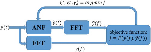
The three ANF parameters $\left[\xi ,{\gamma }_{\omega },{\gamma }_d\right]$ are optimized by minimizing the objective function as

(10) ${\xi }^{\ast },{\gamma }_{\omega }^{\ast },{\gamma }_d^{\ast }=arg\underset{\xi ,{\gamma }_{\omega },{\gamma }_d}{min}J\left(\xi ,{\gamma }_{\omega },{\gamma }_d\right)$(10)

The ANF block with the optimal parameters $\left[{\xi }^{\ast },{\gamma }_{\omega }^{\ast },{\gamma }_d^{\ast }\right]$ is further used in the circadian phase estimation of the actigraphy data.

As addressed above, the convergence, noise rejection, and stability of the ANF need to be ensured by appropriate adaptation rates and damping factor. The frequency components of the ANF outputs around the constant bias, fundamental frequency, and higher harmonics should be equal or close to those of the raw data while the other frequency components are regarded as noise and should be filtered out by the ANF. To achieve this goal, we defined the objective function in the ANF parameter tuning procedure in the following form:

(11) $F\left(y\left(f\right),\tilde{y}\left(f\right);\xi ,{\gamma }_{\omega },{\gamma }_d\right)=J_{harmo}\left(y\left(f\right),\tilde{y}\left(f\right)\right)+J_{noise}\left(y\left(f\right),\tilde{y}\left(f\right)\right)$(11)

where $J_{harmo}$ represents the energy difference around the constant bias, the fundamental and harmonic frequencies between the raw data and ANF outputs. The term $J_{noise}$ represents the energy of the noise in the ANF outputs. This part is introduced in the objective function to minimize the impacts of the noise in the raw data on the circadian phase estimations. Herein, $J_{harmo}$ and $J_{noise}$ are represented explicitly in the following forms:

(12) $J_{harmo}\left(y\left(f\right),\tilde{y}\left(f\right)\right)={\int }_0^{\delta f}{\left[y\left(f\right)-\tilde{y}\left(f\right)\right]}^{2}df+\sum _{n=1}^K{\int }_{n{f}^{\ast }-\delta f}^{n{f}^{\ast }+\delta f}{\left[y\left(f\right)-\tilde{y}\left(f\right)\right]}^{2}df,$(12)

(13) $J_{noise}\left(y\left(f\right),\tilde{y}\left(f\right)\right)=\sum _{n=0}^{K-1}{\int }_{n{f}^{\ast }+\delta f}^{(n+1)f^{\ast }-\delta f}{\tilde{y}}^2\left(f\right)df+{\int }_{K{f}^{\ast }+\delta f}^{+\mathrm{\infty }}{\tilde{y}}^2\left(f\right)df$(13)

where $f^{\ast }$ represents the average fundamental frequency, which is valued at 1/24 (hour⁻¹) as the activity rhythm assessed by actigraphy approximately exhibits a period of 24 h. The term $\delta f$ is the bandwidth of the frequency components around the constant bias and harmonic terms that we want the ANF states to capture. Note that there is no criterion to decide how many frequency components to enter into the ANF states. For the purpose of this paper, we assume that the frequency of the actigraphy is approximately equal to the frequency of the core body temperature. 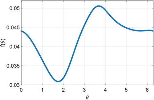The value of $\delta f$ can be decided based on the phase response curve (PRC) in the JFK model (Julius et al. 2019). By checking the raw data measured in the experiment specified in the following section, we find that the light intensity recorded simultaneously with actigraphy is usually ≤1000 lux. All experimental subjects were healthy young adults and followed their daily schedule without large variation in their circadian rhythm during the experiment. The impacts of climate and weather were also excluded in the experimental protocol. Therefore, we assume the circadian phase shift of all of the experimental subjects was induced by light. Based on the phase dynamics of Julius et al. (Julius et al. 2019), when the light intensity is ≤1000 lux, the frequency of the circadian phase in core body temperature is valued at $f\in$[0.0309,0.0506] (hour⁻¹), as shown in Figure 2, which is regarded as the effective frequency components we want ANF to retain. Then we set the bandwidth as = 0.0108 to guarantee that [$f^{\ast }-\delta f,f^{\ast }+\delta f$] in $J_{harmo}$ covers all effective frequency variations, especially those induced by light.

Figure 2. Frequency of phase dynamics of the core body temperature with the light input $I_{max}=$1000 lux based on the JFK model in Julius et al. (Julius et al. 2019)

The objective function given in (11) implies involvement of multi-dimensional nonlinear optimization. The FFT block and ANF state equations make analytically solving the gradient of the objective function to the ANF parameters impractical. To solve this optimization problem, we use a zero-order (gradient-free) optimization method. Reviews in Zakharova and Minashina (Zakharova and Minashina 2015) introduce some widely used zero-order methods to solve the multidimensional optimization problem, including coordinate descent, simplex search, and Hooke-Jeeves ones. However, these methods only enable us to approach the locally optimal solutions from initial guesses. Evolution strategies (ES) algorithm is a population-based, gradient-free, globally optimization method (Beyer and Schwefel 2002), which is developed based on the competition among biological social systems and contains several operators used in the evolutionary algorithm (Trelea 2003), e.g., selection, crossover, mutation, and replacement operators. In this paper, we use the Evolutionary Strategy (ES) algorithm (Ruffio et al. 2011) to optimize the ANF parameters in the parameter tuning process.

Experiment and numerical implementation

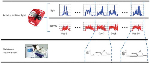
Eight healthy young adult subjects, labeled A3–A10, complied with the experimental protocol, completed the study, and had evaluable data. Three were male and five were female, with ages ranging from 18 to 34 y (mean ± standard deviation: 25.8 ± 6.6 y). This investigation adhered to the Declaration of Helsinki of the World Medical Association and followed the journal’s research guidelines (Portaluppi et al. 2008). It was approved by the University of New Mexico Institutional Review Board and was monitored by the University of New Mexico Health Sciences Center Human Research Protections Office. All subjects provided informed consent. All five female subjects were pre-menopausal, but no effort was made to determine their menstrual phase during the course of the study, since this has been shown not to affect the circadian acrophase nor period of individuals when ambient light, eating schedules, and activity are not controlled (as was the case in this protocol) (Coyne et al. 2000; Ito et al. 1995; Kivelä et al. 1988). Finding of the Morningness-Eveningness Questionnaire (Horne and Ostberg 1976) were as follows: Subjects A3, A4 – intermediate chronotype; Subjects A6, A8 – moderate morning chronotype; Subjects A7, A9 – moderate evening chronotype; Subjects A5, A10 – definite evening chronotype. Although data collection spanned a period of 8 months, the short duration of the protocol shown in Figure 3 for each subject ensured that climate and weather did not play a role, especially since all subjects resided in Albuquerque, New Mexico, known for the stability of its weather (300+ days of sunlight per year). Subjects were asked to wear a GT3X+ Monitor (Actigraph, Pensacola, FL) on the wrist of the non-dominant arm to collect actigraphy continuously at 1 min intervals for 2 weeks. Light intensity was also measured simultaneously by actigraph. Determination of the DLMO took place on the 7th and 14th days of actigraphy monitoring. Saliva samples (~1 mL) were collected at 30 min intervals in dim light (<50 lux) in standard fashion. Approximately 12 to 14 samples were collected per subject, beginning 5 h before the usual (average) bedtime on work or school days (computed from a sleep diary previously completed by the subject) and ending 30 min after the usual (average) bedtime. Samples were collected with SalivaBio Oral Swabs (Salimetrics®, State College, PA) while the subjects lay in a supine position in bed, in dim light (<10 lux, 1800 K). Food and water were consumed only after saliva collection to reduce contamination or dilution of the sample. Participants were instructed to place the swab in their mouth and accumulate saliva for 2 min. After collection, samples were stored at −20 Celsius. For analysis, samples were thawed and centrifuged for 10 min at 2500 rpm, the swabs were removed from the casing, and the supernatant retained. A sensitive direct radioimmunoassay (RIA) using reagents from Buhlmann Laboratories AG (Allschwil, Switzerland) was performed in duplicate on each sample. The assay performance characteristics have been reported by Buhlmann Laboratories AG as follows: Intra-assay Precision (Within-Run): 2.6–20.1%; Inter-assay Precision (Run-to-Run): 6.6–16.7%; Detection Limit: limit of blank (LoB), 0.2 pg/ml; limit of quantitation (LoQ): 0.9 pg/ml (using an intra-assay coefficient of variation (CV) of less than 10%); Dilution Linearity/Parallelism: 93.1%; Spiking Recovery: 106%.

Figure 3. The measurements and experimental procedure

Circadian phase estimation from the melatonin data

We used the DLMO-based assessment of circadian phase shifts between day 7 and day 14 as the baselines for comparison. The timings of the DLMO on day 7 and day 14 are presented as $T_{DLMO,7}$ and, respectively. The reference circadian phase shift between these 2 days is given as

(14) ${\mathrm{\Delta }}_{DLMO}=T_{DLMO,14}-T_{DLMO,7}$(14)

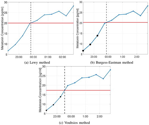
where ${\mathrm{\Delta }}_{DLMO}>0$ means the circadian rhythm in day 14 is delayed compared with that on day 7. Three methods for determining the DLMO are discussed, as demonstrated in Figure 4: (1) Lewy method: measurement of the DLMO by choosing a fixed threshold for every subject and finding the time point once melatonin levels exceed it (Lewy and Sack 1989); (2) Burgess-Eastman method: determining the DLMO by setting the subject’s threshold twice as much as the mean value of his first three low daytime values and finding the time point once melatonin levels exceed it (Burgess and Eastman 2005); and (3) Voultsios method: taking the mean of the subject’s first three low melatonin values plus 2 standard deviations as the threshold (Voultsios et al. 1997). These three methods have been compared (Voultsios et al. 1997), and find in most cases that the Burgess-Eastman and Voultsios methods are more accurate than the Lewy method, since they compensate for individual differences in DLMO thresholds. It is recommended that the fixed threshold of the Lewy method be selected based on the melatonin data of the individual subject; thus, the DLMO thresholds were set as 10 pg/ml, 15 pg/ml, and 40 pg/ml in Lewy & Sack (Lewy and Sack 1989), Lewy et al. (Lewy et al. 1985), and Voultsios et al. (Voultsios et al. 1997), respectively. By checking the melatonin data of the eight subjects, we find that when the fixed threshold is set as 10 pg/ml or 15 pg/ml, we can find the DLMO values (for both day 7 and day 14) of only two subjects and the melatonin levels of almost all subjects remain under 40 pg/ml during the measurement time. However, if we choose 20 pg/ml as the DLMO threshold, the DLMO of four subjects can be found. Hereafter, we set the fixed threshold in Lewy method as 20 pg/ml.

Figure 4. Demonstration of the DLMO measurement methods, where the red horizontal lines show the thresholds to decide the DLMO; the vertical dashed lines mark timings of the DLMO

To distinguish the results of different methods, the DLMO timings on day 7 and day 14 from the three methods specified above are represented as $T_{Lewy,7}$, $T_{Lewy,14}$, $T_{Eastman,7}$, $T_{Eastman,14}$, $T_{Voultsios,7}$, $T_{Voultsios,14}$, respectively. 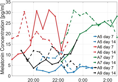The corresponding circadian phase shifts are represented as ${\mathrm{\Delta }}_{Lewy}$, ${\mathrm{\Delta }}_{Eastman}$ and ${\mathrm{\Delta }}_{Voultsios}$, which are listed in Table 1. The notation ‘NaN’ represents the cases when the DLMO measurement method does not work on the melatonin data because the melatonin level remains below the threshold or decreases gradually during the measurement time. We have melatonin data of two-day duration per subject, and thus we have 16 cases to determine the DLMO timing. The Lewy method finds the DLMO timings of eight cases and the circadian phase shift of four subjects (A6 – 8 and A10) while the Burgess-Eastman and Voultsios methods both work for 12 cases and 4 subjects (A3 – 4, A8, A10). The Lewy method uses a fixed threshold for each subject, while the melatonin level for every subject on different days could be different (Voultsios et al. 1997), making this method less feasible to utilize compared with the other two methods. The salivary melatonin profiles of the four subjects for whom both the Burgess-Eastman and Voultsios methods can be utilized to calculate the circadian phase shift are plotted in Figure 5; the individual graphs show melatonin level starts from low levels and increases gradually to reach the DLMO threshold in the following hours. The melatonin profiles of the other four subjects are displayed in Figure 6. It shows three low daytime melatonin values could not be determined in these cases and, as a result, the DLMO thresholds from both Burgess-Eastman and Voultsios methods are ill-defined or too large. However, the DLMO timings of subject A6 and A7 based on the Lewy method can be obtained, since salivary melatonin from these two subjects reaches the 20 pg/ml threshold. The DLMO timings of subject A5 and A7 cannot be determined by all three methods because their melatonin profiles remain at very low levels without a continuous upward trend. The average absolute differences in the circadian phase shifts between these three methods are given in Table 2, where the results from the Lewy method and the Voultsios method agree closely, while the average values of $\left|{\mathrm{\Delta }}_{Lewy}-{\mathrm{\Delta }}_{Eastman}\right|$ and $\left|{\mathrm{\Delta }}_{Eastman}-{\mathrm{\Delta }}_{Voultsios}\right|$ are both more than 50 min.

Table 1. DLMO timings and circadian phase shifts estimated by three different methods

Subjects	$T_{Lewy,7}$	$T_{Lewy,14}$	${\mathrm{\Delta }}_{Lewy}$	$T_{Eastman,7}$	$T_{Eastman,14}$	${\mathrm{\Delta }}_{Eastman}$	$T_{Voultsios,7}$	$T_{Voultsios,14}$	${\mathrm{\Delta }}_{Voultsios}$
A3	NaN	NaN	NaN	19:49	21:14	1:25	19:55	20:52	0:57
A4	NaN	NaN	NaN	19:23	18:29	−0:54	19:36	20:38	1:02
A5	NaN	NaN	NaN	22:07	NaN	NaN	21:53	NaN	NaN
A6	19:55	20:09	0:14	19:54	NaN	NaN	19:33	NaN	NaN
A7	23:49	22:43	−1:06	23:53	NaN	NaN	23:32	NaN	NaN
A8	00:25	01:35	1:10	00:16	01:54	1:38	00:16	01:43	1:27
A9	NaN	NaN	NaN	23:04	NaN	NaN	22:28	NaN	NaN
A10	00:23	22:53	−1:30	23:52	23:43	−0:10	23:37	22:40	−0:57

Table 2. Mean absolute difference of the DLMO results from three different methods, where $\left|{\mathrm{\Delta }}_{Lewy}-{\mathrm{\Delta }}_{Eastman}\right|$ and $\left|{\mathrm{\Delta }}_{Lewy}-{\mathrm{\Delta }}_{Voultsios}\right|$ are the average values of two subjects (A8 and A10), while $\left|{\mathrm{\Delta }}_{Eastman}-{\mathrm{\Delta }}_{Voultsios}\right|$ is the average difference of four subjects (A3, A4, A8, A10)

Methods	$\left|{\mathrm{\Delta }}_{Lewy}-{\mathrm{\Delta }}_{Eastman}\right|$	$\left|{\mathrm{\Delta }}_{Lewy}-{\mathrm{\Delta }}_{Voultsios}\right|$	$\left|{\mathrm{\Delta }}_{Eastman}-{\mathrm{\Delta }}_{Voultsios}\right|$
Difference	0:54	0:25	0:51

Figure 5. Salivary melatonin profiles of four subjects (A3−4, A8, A10)

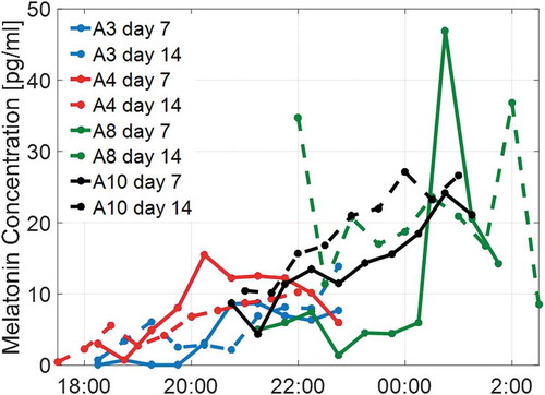
Figure 6. Salivary melatonin profiles of four subjects (A5−7, A9)

Circadian phase estimation from the actigraphy data by ANF

The actigraphy data of every subject collected during the 2 weeks are imported into the parameter tuning process in Figure 1, and the globally optimal ANF parameters for each subject are calculated by the ES algorithm. Note that the ANF orders and the initial values of ANF states and frequency in (2) and (3) all affect the ANF parameters and estimation results. Firstly, we use the ANF with only the first harmonic term, i.e., we set $K=1$ in (4), and define the initial values of the ANF states and frequency as

$x\left(0\right)={\left[0,0,0\right]}^T,\omega \left(0\right)=\frac{2\pi }{24},$

which implies that the initial harmonic terms and constant bias in the ANF states are all 0, and the initial frequency corresponds to a 24 h period. The optimal ANF parameters of the eight subjects are listed in Table 3. The optimal damping factors ${\xi }^{\ast }$ of the eight subjects are valued between 0.0743 and 0.1914. Compared with the optimal adaptation rates of the constant bias ${\gamma }_d^{\ast }$, the optimal adaptation rates of fundamental frequency ${\gamma }_{\omega }^{\ast }$ are much smaller. That is because the initial constant biases in the ANF are 0 while the mean actigraphy values of all subjects are about 1000, suggesting that larger adaptation should be added into the constant bias in the ANF states. However, the initial frequency in the ANF (2π/24) is close to the fundamental frequency of the human activity rhythm determined by actigraphy. 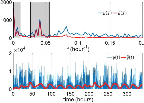The term $J_{noise}$ in the objective function also prevents large variations in the estimated fundamental frequency. Therefore, the optimal adaptation rates in the fundamental frequency cannot be too large. Figure 7 compares the ANF outputs with the optimal parameters to the raw data in frequency and time domains, the gray-shaded regions showing the frequency components considered in $J_{harmo}$. We observe the ANF with optimal parameters makes $\tilde{y}\left(f\right)$ close to in the gray regions and, at the same time, decreases the amplitude of $\tilde{y}\left(f\right)$ outside them. The lower subfigure also demonstrates that $\tilde{y}\left(t\right)$accurately follows the constant bias and first harmonics of $y\left(t\right)$ and has filtered out the noise in other frequencies.

Table 3. Optimal ANF parameters from the ES algorithm

Subjects	${\xi }^{\ast }$	${\gamma }_{\omega }^{\ast }$	${\gamma }_d^{\ast }$
A3	0.1251	3.8019$\times$10^−9	0.0339
A4	0.1232	8.3313$\times$10^−23	0.0491
A5	0.1914	4.6079$\times$10^−9	0.0394
A6	0.0743	3.4765$\times$10^−22	0.0641
A7	0.0965	7.7570$\times$10^−22	0.0544
A8	0.1287	2.5755$\times$10^−22	0.0357
A9	0.1019	6.2113$\times$10^−10	0.0269
A10	0.0862	1.5826$\times$10^−22	0.0556

Figure 7. Comparison of the raw data (blue) and ANF results (red) with optimal ANF parameters of subject A3 in the frequency domain (upper subfigure) and time domain (lower subfigure)

We apply the ANF with optimal parameters in Table 3 on the actigraphy data of the corresponding subject and generate the values of the circadian phase as $\theta \left(t\right)$ from the ANF states by (8). The circadian phase shift between day 7 and day 14 is calculated from by

(15) ${\mathrm{\Delta }}_{ANF}=\frac{1}{2\pi }{\int }_0^{24}\theta \left(t+6\times 24\right)-\theta \left(t+13\times 24\right)dt$(15)

where $t=6\times 24$ (hours) and $t=13\times 24$ (hours) represent the beginning of day 7 and day 14. The circadian phase shift estimation results from the ANF, and their comparison with the DLMO results are listed in Table 4. Compared with the DLMO methods, the ANF can estimate the circadian phase shifts from the actigraphy data of all eight cases. However, the circadian phase shifts estimated from the first-order ANF (${\mathrm{\Delta }}_{ANF}$) are still far away from the DLMO results in several cases, e.g., the difference in ${\mathrm{\Delta }}_{ANF}$ and ${\mathrm{\Delta }}_{Lewy}$ is even more than 1.5 h in the case of subject A10.

Table 4. Circadian phase shift estimation results (hours) from the DLMO method and first-order ANF with optimal parameters. Values in parentheses give the deviations of ${\mathrm{\Delta }}_{ANF}$ from the DLMO results

Subjects	${\mathrm{\Delta }}_{Lewy}$	${\mathrm{\Delta }}_{Eastman}$	${\mathrm{\Delta }}_{Voultsios}$	${\mathrm{\Delta }}_{ANF}$
A3	NaN	1:25 (1:37)	0:57 (1:09)	−0:12
A4	NaN	−0:54 (−0:40)	1:02 (1:16)	−0:14
A5	NaN	NaN	NaN	−1:22
A6	0:14 (−0:30)	NaN	NaN	0:44
A7	−1:06 (−0:22)	NaN	NaN	−0:34
A8	1:10 (0:27)	1:38 (0:55)	1:27 (0:44)	0:43
A9	NaN	NaN	NaN	−1:56
A10	−1:30 (−1:52)	−0:10 (−0:32)	−0.57 (−1:19)	0:22

Impacts of ANF orders on estimation results

The ANF with the first harmonic states captures the frequency components around $f^{\ast }$ and constant bias, as shown in Figure 7. However, the higher harmonic terms in the raw data may have large amplitudes in many cases, which could affect the circadian phase estimation results. We increase the value of $K$ in (4) to increase the ANF orders and incorporate the higher harmonics into the estimation results. The parameter tuning process is performed on the higher-order ANF and their optimal ANF parameters in subject A3 are listed in Table 5, where we can observe that all three optimal parameters decrease gradually with the increasing ANF order.

Table 5. Optimal ANF parameters of subject A3 with various numbers of ANF orders

ANF orders	${\xi }^{\ast }$	${\gamma }_{\omega }^{\ast }$	${\gamma }_d^{\ast }$
1	0.1251	3.8019$\times$10^−9	0.0339
2	0.0904	2.0534$\times$10^−9	0.0334
3	0.0750	4.9957$\times$10^−10	0.0333
4	0.0667	3.5233$\times$10^−10	0.0329
5	0.0599	2.0893$\times$10^−10	0.0324

The results of $\tilde{y}\left(t\right)$ from different orders of ANF are plotted in Figure 8, where $\tilde{y}\left(t\right)$ from higher-order ANF captures the higher harmonics and oscillates more frequently. As the ANF order increases, the ANF output $\tilde{y}\left(t\right)$ approaches the raw data $y\left(t\right)$, which demonstrates that the adaptation rates of the fundamental frequency, constant bias, and the damping factor can be set to lower values. The ANF states $x_1\left(t\right)$ from different orders of ANF plotted in the middle subfigure in Figure 8 shows that the profile of $x_1\left(t\right)$ is very similar to a clear sinusoidal wave when the ANF order is large enough. Figure 9 demonstrates the minute-by-minute estimated phase shift $\psi \left(t\right)$ with respect to day 7 of six subjects (A3-4, A6-8, A10) from different orders of ANF and the comparison with DLMO results, where the estimated phase shift is defined as

(16) $\begin{array}{rl}& \psi \left(t\right)=t-\frac{24\cdot \theta \left(t\right)}{2\pi }-{\int }_{6\times 24}^{7\times 24}\left[\tau -\frac{24\cdot \theta \left(\tau \right)}{2\pi }\right]d\tau ,t\\ & \in \left[6\times 24,14\times 24\right].\end{array}$(16)

Figure 8. Estimated actigraphy values (upper), first ANF states (middle), and circadian phases (lower) from different orders of ANF with optimal parameters

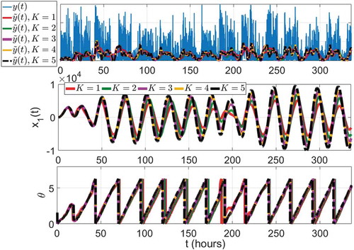
Figure 9. Estimated phase shift from day 7 to day 14 from first (red), second (green), third (cyan), fourth (yellow), and fifth (black) order ANF, where the minute-by-minute estimated phase shift $\psi \left(t\right)$ is defined in (16). The horizontal lines in the last day mark the average phase shift between day 7 and day 14. The blue lines show the phase shift estimated from the DLMO methods (Lewy –, Burgess-Eastman – - -, Voultsios – – –)

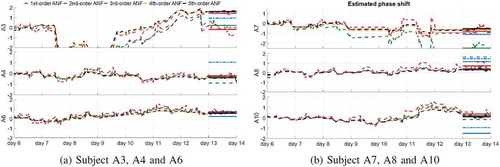
Note that the circadian phase $\theta \left(t\right)$ used in this function should be unwrapped and

${\mathrm{\Delta }}_{ANF}={\int }_{13\times 24}^{14\times 24}\psi \left(\tau \right)/24d\tau$

In subjects A6 and A10, as the ANF order increases, the value of ${\mathrm{\Delta }}_{ANF}$ moves toward the DLMO results, while in A8, ${\mathrm{\Delta }}_{ANF}$ moves slightly far from the three DLMO results as the ANF order increases. In other cases, the DLMO results may lie between the values ${\mathrm{\Delta }}_{ANF}$ from different ANF orders (A3 and A7) or the difference in ${\mathrm{\Delta }}_{Eastman}$ and ${\mathrm{\Delta }}_{Voultsios}$ is too large (A4).

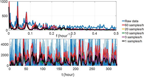
Because of the application herein is related to the circadian rhythm, the fundamental frequency of the ANF is around 1/24 h⁻¹. If we consider the first five harmonics, the bandwidth of the data is 5/24 h⁻¹. Nyquist Sampling Theorem dictates that the theoretical minimum sampling frequency is 10/24 h⁻¹. However, because of the non-ideal filtering, we consider a higher limit of 100/24 h⁻¹ = 4.16 h⁻¹ (Butkov and Teofilo 2007). The sampling frequency of the raw actigraphy data is 60 samples/h, which is much higher than the practical sampling limit. We use numerical simulations to illustrate the effect of sampling frequency on the ANF estimation of results. We fix the damping factor and adaptation rates and gradually decrease the sampling rate (downsampling by interpolation) and compare the ANF estimation results of $\tilde{y}\left(t\right)$ in time and frequency domains. Figure 10 shows the ANF estimation outputs of $\tilde{y}\left(t\right)$ with various sampling rates. For the estimated phase comparison, denote the circadian phase shifts $\psi \left(t\right)$ of 60 samples/h, 30 samples/h, 20 samples/h, 10 samples/h, 5 samples/h, 3 samples/h and 1 sample/h by ${\psi }_{60}\left(t\right)$, ${\psi }_{30}\left(t\right)$, ${\psi }_{20}\left(t\right)$, ${\psi }_{10}\left(t\right)$, ${\psi }_5\left(t\right)$,, and ${\psi }_1\left(t\right)$, respectively. Using ${\psi }_{60}\left(t\right)$ as the baseline for comparison, Table 6 lists the root-mean-square error (RMSE) between the estimated circadian phase shifts using the data of the different sampling frequencies. When the sampling frequency is ≥10 samples/h, the difference in the circadian phase shifts is ≤15 min. Therefore, we recommend at least 10 samples/h to ensure the accuracy of the ANF circadian phase shift estimation.

Table 6. Difference between circadian phase shift estimation results of actigraphy data with various sampling frequencies

Phase shift difference	minutes
${\psi }_{60}\left(t\right)-{\psi }_{30}\left(t\right)$	9.41
${\psi }_{60}\left(t\right)-{\psi }_{20}\left(t\right)$	8.31
${\psi }_{60}\left(t\right)-{\psi }_{10}\left(t\right)$	14.08
${\psi }_{60}\left(t\right)-{\psi }_5\left(t\right)$	21.20
${\psi }_{60}\left(t\right)-{\psi }_3\left(t\right)$	32.68
${\psi }_{60}\left(t\right)-{\psi }_1\left(t\right)$	58.72

Figure 10. ANF estimation results in time and frequency domains with different sampling frequencies in actigraphy data of subject A3

The average absolute difference between the circadian phase shifts derived from actigraphy by ANF and those derived from DLMO are listed in Table 7. When the ANF order is ≥3, the average differences in the circadian phase shifts by ANF and those from DLMO in the Lewy, Burgess-Eastman, and Voultsios methods are about 50 min, 34 min, and 65 min, respectively, which implies that the results of ${\mathrm{\Delta }}_{ANF}$ are more consistent with ${\mathrm{\Delta }}_{Eastman}$, especially when the ANF order is high enough. The ANF order for circadian phase estimation is determined based on the trade-off between the algorithm complexity, convergence rate, and accuracy of the circadian phase estimate. Figure 8 and Figure 9 show that the ANF estimate, $\tilde{y}\left(t\right)$, and circadian phase estimate, $\psi \left(t\right)$, have almost converged for K ≥ 3. Higher ANF order increases computational complexity and increases convergence time, as shown in Table 8 (calculated by the method of Zhang et al. (Zhang et al. 2012, 2013) with adaptation rates and damping factors in Table 5). We, therefore, choose K = 3 in this paper.

Table 7. Average absolute difference of circadian phase shifts from DLMO and ANF with optimal parameters

Orders	$\left|{\mathrm{\Delta }}_{Lewy}-{\mathrm{\Delta }}_{ANF}\right|$	$\left|{\mathrm{\Delta }}_{Eastman}-{\mathrm{\Delta }}_{ANF}\right|$	$\left|{\mathrm{\Delta }}_{Voultsios}-{\mathrm{\Delta }}_{ANF}\right|$
1	0:50	0:56	1:07
2	1:04	0:51	1:04
3	0:47	0:32	1:01
4	0:48	0:34	1:03
5	0:50	0:34	1:05

Table 8. Convergence rates and convergence time (error decreases to 5% of initial error) of different order ANFs

K	1	2	3	4	5
Convergence rate	$e^{-\frac{t}{31.80h}}$	$e^{-\frac{t}{41.01h}}$	$e^{-\frac{t}{49.43h}}$	$e^{-\frac{t}{56.01h}}$	$e^{-\frac{t}{62.75h}}$
Convergence time (days)	3.88	5.12	6.17	6.99	7.83

The circadian phase shift estimation results of the third-order ANF are listed in Table 9. Compared with Table 4, the value of ${\mathrm{\Delta }}_{ANF}$ varies most dramatically in subject A3, changing from an advance of 12 min to a delay of 1 h and 25 min, shifting more closely to ${\mathrm{\Delta }}_{Voultsios}$ and ${\mathrm{\Delta }}_{Eastman}$. In addition, the average values of $\left|{\mathrm{\Delta }}_{Lewy}-{\mathrm{\Delta }}_{ANF}\right|$, $\left|{\mathrm{\Delta }}_{Eastman}-{\mathrm{\Delta }}_{ANF}\right|$ and $\left|{\mathrm{\Delta }}_{Voultsios}-{\mathrm{\Delta }}_{ANF}\right|$ (32–61 min) are also close to the differences between these three DLMO methods (25–54 min) given in Table 2. As discussed by Ancoli-Israel et al. (Ancoli-Israel et al. 2003), the phases and period of the actigraphy-based estimated bedtime and wake-up time are highly consistent with those from melatonin secretion. Our results, therefore, demonstrate that minute-by-minute actigraphy can reliably estimate the circadian phase shift, and its estimation results are correlated with those derived from the DLMO.

Table 9. Circadian phase shift estimation results from the DLMO method and third-order ANF with optimal parameters. Values in parentheses give the deviations of ${\mathrm{\Delta }}_{ANF}$ from the DLMO results

Subjects	${\mathrm{\Delta }}_{Lewy}$	${\mathrm{\Delta }}_{Eastman}$	${\mathrm{\Delta }}_{Voultsios}$	${\mathrm{\Delta }}_{ANF}$
A3	NaN	1:25 (0:00)	0:57 (−0:28)	1:25
A4	NaN	−0:54 (−0:33)	1:02 (1:23)	−0:21
A5	NaN	NaN	NaN	−0:17
A6	0:14 (−0:25)	NaN	NaN	0:39
A7	−1:06 (−0:18)	NaN	NaN	−0:48
A8	1:10 (0:48)	1:38 (1:16)	1:27 (1:05)	0:22
A9	NaN	NaN	NaN	−1:04
A10	−1:30 (−1:39)	−0:10 (−0:19)	−0:57 (−1:06)	0:09

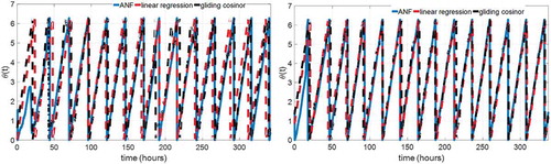
Two methods have been traditionally used for computation of the phase of rhythm based on the actogram method (Refinetti et al. 2007). The daily circadian activity onsets are most often used as phase markers to fit the circadian period (Herzog et al. 2004). The second method is the gliding cosinor method, which fits a cosine curve to the data by least squares regression (Teicher and Barber 1990). We apply the linear regression of the phase markers and gliding cosinor method on the actigraphy data. The estimated circadian phases from ANF, linear regression, and gliding cosinor of subject A3 and A4 are plotted in Figure 11. Average absolute deviations of estimated circadian phase shifts in all eight subjects of ANF, linear regression, and gliding cosinor from the DLMO results are listed in Table 10, where the third-order ANF estimation results are closer to those of the three DLMO methods than the linear regression of activity onsets and gliding cosinor method. The linear regression of phase markers and gliding cosinor method need to use batches of data (of 24 h in duration for our simulation) to fit the circadian period and phase, while the ANF algorithm has the capability to estimate the circadian phase online (simultaneously with the measurement of data). Therefore, the ANF algorithm is more accurate and amenable to online implementation in estimating the circadian phase from actigraphy data than circadian phase markers and gliding cosinor method. Also, the ANF algorithm used in the circadian phase (shift) estimation should be well formulated. The estimation accuracy of the circadian phase (shift) obtained from the actigraphy data by ANF can be improved by the parameter tuning process proposed in this paper.

Table 10. Average absolute difference of circadian phase shifts of all eight subjects from ANF, linear regression of phase maker, gliding cosinor, and DLMO methods

Methods	Lewy method	Burgess-Eastman method	Voultsios method
3rd-order ANF	0:47	0:32	1:01
Linear regression	1:05	1:18	1:36
Gliding cosinor	1:50	1:08	1:13

Figure 11. Comparison of circadian phase estimation results from ANF, linear regression of phase markers, and gliding cosinor of subject A3 (left) and A4 (right)

Conclusion

This paper proposes a parameter tuning process for the ANF algorithm for use to determine circadian phase shift estimation from minute-by-minute actigraphy data. The objective function is defined based on the frequency distribution of the raw data and ANF output. The optimal ANF parameters, including both adaptation rates and damping factor, are solved by minimizing the proposed objective function. The simulation results on the experimental data show that the circadian phase shifts obtained from actigraphy by ANF are very consistent with the results obtained from the DLMO method of Burgess-Eastman, especially when the ANF contains high harmonic terms. These results imply that the ANF algorithm, with appropriate parameters, can function well to estimate circadian phase shift, and actigraphy data, the measurement of which is more convenient than DLMO, can be of utility for circadian phase shift estimation.

Acknowledgements

This work was supported by the National Science Foundation (NSF) through the Smart Lighting Engineering Research Center (EEC-0812056) and in part by the Army Research Office through Grant number W911NF-17-1-0562 and by New York State under NYSTAR contract C130145. The authors would like to thank Dr. Jiaxiang Zhang for his contribution to the initial portion of this research as part of his doctoral research and to the staff of the University of New Mexico Hospital Sleep Disorders Center who carried out the DLMO procedures: Steven Lopez, Alex Valdez, Cielo Ortiz, and Ryan Valdez.

Additional information

Funding

This work was supported by the Army Research Office [W911NF-17-1-0562]; National Science Foundation [EEC-0812056]; New York State Foundation for Science, Technology and Innovation [C130145].

References

- Ancoli-Israel S, Cole R, Alessi C, Chambers M, Moorcoroft W, Pollak CP. 2003. The role of actigraphy in the study of sleep and circadian rhythms. Sleep. 26:342–392. doi:10.1093/sleep/26.3.342
- Beyer HG, Schwefel HP. 2002. Evolution strategies − a comprehensive introduction. Nat Comput. 1:3–52. doi:10.1023/A:1015059928466
- Burgess HJ, Eastman CI. 2005. The dim light melatonin onset following fixed and free sleep schedules. J Sleep Res. 14:229–237. doi:10.1111/j.1365-2869.2005.00470.x
- Butkov N, Teofilo L. 2007. Fundamentals of sleep technology. Philadelphia, PA: Lippincott Williams & Wilkins.
- Coyne MD, Kesick CM, Doherty TJ, Kolka MA, Stephenson LA. 2000. Circadian rhythm changes in core temperature over the menstrual cycle: method for noninvasive monitoring. Am J Physiol Regul Integr Comp Physiol. 279:R1316–1320. doi:10.1152/ajpregu.2000.279.4.R1316
- Crowley SJ, Suh C, Molina TA, Fogg LF, Sharkey KM, Carskadon MA. 2016. Estimating the dim light melatonin onset of adolescents within a 6-h sampling window: the impact of sampling rate and threshold method. Sleep Med. 20:59–66. doi:10.1016/j.sleep.2015.11.019
- Forger DB, Jewett ME, Kronauer RE. 1999. A simpler model of the human circadian pacemaker. J Biol Rhythms. 14:532–537. doi:10.1177/074873099129000867
- Forger DB, Peskin CS. 2003. A detailed predictive model of the mammalian circadian clock. Proc Natl Acad Sci USA. 100:14806–14811. doi:10.1073/pnas.2036281100
- Herzog ED, Aton SJ, Numano R, Sakaki Y, Tei H. 2004. Temporal precision in the mammalian circadian system: a reliable clock from less reliable neurons. J Biol Rhythms. 19(1):35–46. doi:10.1177/0748730403260776
- Horne JA, Ostberg O. 1976. A self-assessment questionnaire to determine morningness-eveningness in human circadian rhythms. Int J Chronobiol. 4:97–110. PMID: 1027738
- Hsu L, Ortega R, Damm G. 1999. A globally convergent frequency estimator. IEEE Trans Autom Control. 44:698–713. doi:10.1109/9.754808
- Ito M, Kohsaka M, Honma K, Fukuda N, Honma S, Katsuno Y, Kawai I, Honma H, Morita N, Miyamoto T. 1995. Changes in biological rhythm and sleep structure during the menstrual cycle in healthy women. Seishin Shinkeigaku Zasshi. 97:155–164. PMID: 7777641
- Jewett ME, Forger DB, Kronauer RE. 1999. Revised limit cycle oscillator model of human circadian pacemaker. J Biol Rhythms. 14:493–499. doi:10.1177/074873049901400608
- Julius A, Zhang J, Qiao W, Wen JT. 2016. Multi-input adaptive notch filter and observer for circadian phase estimation. Int J Adapt Control. 30:1375–1388. doi:10.1002/acs.2659
- Julius A, Zhang J, Wen JT. 2019. Time optimal entrainment control for circadian rhythm. PLoS ONE. 14(12):e0225988. doi:10.1371/journal.pone.0225988
- Kivelä A, Kauppila A, Ylöstalo P, Vakkuri O, Leppäluoto J. 1988. Seasonal, menstrual and circadian secretions of melatonin, gonadotropins and prolactin in women. Acta Physiol Scand. 132:321–327. doi:10.1111/j.1748-1716.1988.tb08335.x
- Knutsson A. 2003. Health disorders of shift workers. Occup Med (Lond). 53:103–108. doi:10.1093/occmed/kqg048
- Kronauer RE, Forger DB, Jewett ME. 1999. Quantifying human circadian pacemaker response to brief, extended, and repeated light stimuli over the phototopic range. J Biol Rhythms. 14:501–516. doi:10.1177/074873049901400609
- LeBourgeois MK, Carskadon MA, Akacem LD, Simpkin CT, Wright KP, Achermann P, Jenni OG. 2013. Circadian phase and its relationship to nighttime sleep in toddlers. J Biol Rhythms. 28:322–331. doi:10.1177/0748730413506543
- Lewy AJ, Sack RL. 1989. The dim light melatonin onset as a marker for circadian phase position. Chronobiol Int. 6:93–102. doi:10.3109/07420528909059144
- Lewy AJ, Sack RL, Singer CM. 1985. Immediate and delayed effects of bright light on human melatonin production: shifting “dawn” and “dusk” shifts the dim light melatonin onset (dlmo). Ann NY Acad Sci. 453:253–259. doi:10.1111/j.1749-6632.1985.tb11815.x
- Lu Z, Klein-Cardena K, Lee S, Autonsen TM, Girvan M, Ott E. 2016. Resynchronization of circadian oscillators and the east-west asymmetry of jetlag. Chaos. 26:094811. doi:10.1063/1.4954275
- Mojiri M, Karimi-Ghartemani M, Bakhshai A. 2007. Time-domain signal analysis using adaptive notch filter. IEEE Trans Signal Process. 55:85–93. doi:10.1109/TSP.2006.885686
- Portaluppi F, Touitou Y, Smolensky MH. 2008. Ethical and methodological standards for laboratory and medical biological rhythm research. Chronobiol Int. 25:999–1016. doi:10.1080/07420520802544530
- Qiao W, Wen JT, Julius A. 2017. Entrainment control of phase dynamics. IEEE Trans Autom Control. 63:445–450. doi:10.1109/TAC.2016.2555885
- Refinetti R, Lissen GC, Halberg F. 2007. Procedures for numerical analysis of circadian rhythms. Biol Rhythm Res. 38(4):275–325. doi:10.1080/09291010600903692
- Ruffio E, Saury D, Petit D, Girault M. 2011. Tutorial 2: zero-order optimization algorithms. Semantic Scholar. https://www.semanticscholar.org/paper/Tutorial-2-%3A-Zero-Order-optimization-algorithms-Ruffio-Saury/f3b4e17cdc5724a6064d6126e2dbfe86bf7ef742
- Serkh K, Forger DB. 2014. Optimal schedules of light exposure for rapidly correcting circadian misalignment. PLoS Comput Biol. 10:e1003523. doi:10.1371/journal.pcbi.1003523
- Smolensky MH, Hermida RC, Reinberg A, Sackett-Lundeen L, Portaluppi F. 2016. Circadian disruption: new clinical perspective of disease pathology and basis for chronotherapeutic intervention. Chronobiol Int. 33(8):1101–1119. doi:10.1080/07420528.2016.1184678
- Swaab DF, Filers E, Partiman TS. 1985. The suprachiasmatic nucleus of the human brain in relation to sex, age and senile dementia. Brain Res. 342:37–44. doi:10.1016/0006-8993(85)91350-2
- Teicher MH, Barber NI. 1990. Cosifit: an interactive program for simultaneous multioscillator cosinor analysis of time-series data. Comput Biomed Res. 23(3):283–295. doi:10.1016/0010-4809(90)90022-5
- Trelea IC. 2003. The particle swarm optimization algorithm: convergence analysis and parameter selection. Inf Process Lett. 85:317–325. doi:10.1016/S0020-0190(02)00447-7
- Verwey M, Robinson B, Amir S. 2013. Recording and analysis of circadian rhythms in running-wheel activity in rodents. J Vis Exp. 71:50186. doi:10.3791/50186
- Voultsios A, Kennawlay DJ, Dawson D. 1997. Salivary melatonin as a circadian phase marker: validation and comparison to plasma melatonin. J Biol Rhythms. 12:457–466. doi:10.1177/074873049701200507
- Winfree AT. 2001. The geometry of biological time. Berlin, Germany: Springer.
- Woelders T, Beersma DG, Gordijn MC, Hut RA, Wams EJ. 2017. Daily light exposure patterns reveal phase and period of the human circadian clock. J Biol Rhythm. 32(3):274–286. doi:10.1177/0748730417696787
- Zakharova EM, Minashina IK. 2015. Review of multidimensional optimization. J Commun Technol El. 60:625–636. doi:10.1134/S1064226915060194
- Zhang J, Wen JT, Julius A. 2012. Adaptive circadian rhythm estimator and its application to locomotor activity. The conference paper in 2012 IEEE Signal Process Med Biol Symp, pp. 1–6, NY, USA. doi:10.1109/SPMB.2012.6469471
- Zhang J, Wen JT, Julius A. 2013. Adaptive circadian argument estimator and its application to circadian argument control. The conference paper in 2013 Proc Am Control Conf, pp. 2295–2300, Washington DC. doi:10.1109/ACC.2013.6580176
- Zhang J, Qiao W, Wen JT, Julius A. 2016. Light-based circadian rhythm control: entrainment and optimization. Automatica. 68:44–55. doi:10.1016/j.automatica.2016.01.052