Cellular coupling determines scale-invariant behavior of neurons in suprachiasmatic nucleus

ABSTRACT

The main clock in mammals, located in the suprachiasmatic nucleus (SCN) of hypothalamus, not only regulates the daily rhythms in physiological and behavioral activities, but also plays a key role as one of the control nodes in the brain regulating behavioral activity. As such, it induces scale-invariance in the temporal patterns of behavioral activity and of multi-unit neural activity of the SCN network. In particular, the scale-invariant patterns maintain across multiple time scales from 3 minutes to 10 hours, characterized by a scaling exponent around 1. Thus far, no study found the origin of the scale-invariance of the SCN network. Using the method of correlation-dependent balance estimation of diffusion entropy (cBEDE), we found that scale-invariance also exists in the individual neurons of the SCN, and the scale invariance properties are significantly increased when the neurons are coupled in a network of neurons. Improved scale invariance in the single neurons is, therefore, imposed by the emergent network properties of the SCN network. Our findings show that the scale-invariance of the SCN can already be found at the level of the individual neurons and that the application of a scale invariance measure, such as cBEDE, can help in determining the network status of the SCN.

KEYWORDS:

• Circadian rhythm
• diffusion entropy
• scale-invariance
• single-cell
• suprachiasmatic nucleus

Introduction

The main clock, which is located in the suprachiasmatic nucleus (SCN) of hypothalamus, regulates the circadian (~24 h) rhythms in physiology and behavior in mammals (Vansteensel et al. 2008; Welsh et al. 2010). As such, the SCN has been identified as one of the control nodes in the brain regulating normal behavioral activity (Hu et al. 2007). This activity is characterized by a fractal, or scale invariant, organization over a wide range of time scales. Scale invariance is thought to be a measure for the optimal balance in the brain between flexibility and rigidity (Gu et al. 2019). Using the method of Detrended Fluctuation Analysis (DFA), a scaling exponent can be obtained from time series data which evaluates correlations in fluctuations over time. A scaling exponent of 1 indicates the optimal balance between flexibility and rigidity, while a scaling exponent of 0.5 indicates uncorrelated randomness, and that of 1.5 indicates overly rigid regularity (Gu et al. 2015). In control animals, the scaling exponent found in experimental data from behavioral activity was characterized by a scaling-exponent of ~1.0, and is maintained over multiple timescales from 3 min up to ~10 h (Hu et al. 2007, 2009). Dysfunction of the SCN disrupts these scale invariant patterns. A cross-over point emerges with intact scale invariant patterns (scaling exponent ~1) from 3 min to ~1.5 h for humans (Hu et al. 2009) and to ~4 h for rats (Hu et al. 2007) and a scaling component of 0.5 from the cross-over point up to ~10 h. The emergence of this break suggests that the SCN controls the time scale from several hours (1.5 h for human and 4 h for rat) to at least ~10 h in the temporal patterns of behavioral activity. Note that the length of the data recordings have not enabled investigation of time scales longer than 10 h.

The scale-invariant behavior has also been found in the patterns of the multi-unit electrical activity (MUA) of the SCN network, itself, using the DFA method (Hu et al. 2012). Both the range of the scale-invariant scales and the scaling exponents for the MUA are close to the ones found for behavioral activity, i.e., the range is from min up to 10 h, and the exponent is ~1. This finding supports the view that the SCN is involved in the regulation of scale-invariance in the patterns of behavioral activity.

These studies have shown that the brain network is important for optimal functioning of the circadian system. To investigate this network more, it is necessary to also investigate the building blocks for the SCN network, the single cells, and their interconnections. Unfortunately, no study has explored whether scale-invariant patterns exist in single SCN neurons or whether coupling between the neurons plays a role in scale-invariance. In this article, we examined the scale-invariant patterns for single SCN neurons as well as the role of coupling between these neurons for scale-invariance. Bioluminescence traces of single neurons were used as previously reported (Abel et al. 2016). To reduce the coupling between the neurons, tetrodotoxin (TTX) was applied, and to restore the coupling the TTX was washed out (Abel et al. 2016). Because the length of the time series for the bioluminescence reporter data is much shorter than the time series coming from behavioral recordings or electrical activity recordings, DFA may not be suitable for these analyses. With only ~200 data points in the bioluminescence time series, the application of DFA may lead to misleading results, because DFA requires the length of the time series to be larger than ~1000 (Ren et al. 2018). Accordingly, a method which is tailored to measure scale-invariance in shorter time series (with a minimum of only around 100 data points), is correlation-dependent balance estimation of diffusion entropy (cBEDE), which is applied in the present study (Pan et al. 2014a, 2014b; Qi and Yang 2011; Zhang et al. 2012).

The rest of the article is organized as follows. Section II introduces the bioluminescence reporter time series and the cBEDE method. In Section III, the results, including the scaling-invariant behaviors in both the single neurons and the SCN network, are compared between the different conditions, during the application of TTX and after the washout of TTX. In addition, we also examined the scale-invariant behaviors for the shuffled data. Finally, the conclusions and the discussions are presented in Section IV.

Data description and methods

Data description

We selected bioluminescence reporter data of four distinct SCN mouse explants, each of which contains ~400 cells. The data were recorded each hour either during TTX application or after washout of TTX (Abel et al. 2016). The experimental process lasted 6 d during TTX application; therefore, the length of the time series was ~140 data points. After these 6 d, the recordings lasted for an additional 8 − 12 d in the stage when TTX was washed out. In order to remove the aftereffects of TTX on SCNs, the data of the first 48 h after washout of TTX was not taken into account, which resulted in the time series to be composed of ~140-230 data points.

For comparison, we also examined the scale-invariant behavior in so-called shuffled time series. The shuffled data were obtained as follows: In a time series, the position of each data point in the time series was exchanged with the position of a randomly selected data point. Therefore, in the shuffled time series, the data values are the same, but the organization of the data are different from the original time series. For each phase, the TTX phase and the washout phase, this was done separately for each time series.

Methods

The method of correlation-dependent balance estimation of diffusion entropy (cBEDE) is used to examine the scale-invariance of entropy in short stationary time series or non-stationary time series after removing any trend. In this section, we introduce the definition of the scale-invariance, and how to de-trend the data, the method of Diffusion Entropy, and the methods of Diffusion Entropy Analysis (DEA) and cBEDE, which are developed from the method of Diffusion Entropy. The details for the method of Diffusion Entropy, DEA, and cBEDE can be found elsewhere (Feng et al. 2019; Grigolini et al. 2001; Pan et al. 2014a, 2014b; Qi and Yang 2011; Zhang et al. 2012).

1) Definition of scale-invariance: For a stochastic placement $x$ at time $t$, we use $p\left(x,t\right)$ to represent its probability distribution function (PDF), which could describe the stochastic process of $x$. If $p\left(x,t\right)$ satisfies:

(1) $p\left(x,t\right)\text{~}\frac{1}{t^{\delta }}F\left(\frac{x}{t^{\delta }}\right)$(1)

The stochastic process behaves scale-invariant, where $\delta$ and $F(\cdot )$ represents the scaling exponent and a function, respectively. If $\frac{x}{t^{\delta }}$ is replaced by $x\mathrm{p}\left(\mathrm{x},\mathrm{t}\right)\text{~}\frac{1}{{\mathrm{t}}^{\alpha }}\mathrm{F}\left(\frac{\mathrm{x}}{{\mathrm{t}}^{\alpha }}\right)$, $p\left(x,t\right)$ remains unchanged. Accordingly, the Shannon entropy reads,

(2) $S\left(t\right)\equiv -\underset{-\mathrm{\infty }}{\overset{+\mathrm{\infty }}{\int }}p\left(x,t\right)\mathrm{l}\mathrm{n}\left[p\left(x,t\right)\right]d\left(x\right)=A+\delta \mathrm{l}\mathrm{n}\left(t\right)$(2)

Eq. (2)(2) $S\left(t\right)\equiv -\underset{-\mathrm{\infty }}{\overset{+\mathrm{\infty }}{\int }}p\left(x,t\right)\mathrm{l}\mathrm{n}\left[p\left(x,t\right)\right]d\left(x\right)=A+\delta \mathrm{l}\mathrm{n}\left(t\right)$(2) stands for any form of the probability distribution function. Hence, the slope for the linear relationship of entropy versus natural logarithm of time scales are an unbiased estimation of the scaling exponent. A scaling exponent of $\delta >0.5$ represents a fractal with a persistent behavior, while $\delta <0.5$ represents a non-persistent behavior (Carbone et al. 2004; Li 2010; Li and Li 2017; Mäkikallio et al. 1999).

2) Removing the trend of the data: Before we calculate the scale-invariant behaviors of SCN neurons, the raw time series $Y=\left\{y_1,y_2,\dots ,y_N\right\}$ obtained from the experiment (Abel et al. 2016) must be de-trended, where $N$ represents the length of the time series (Zhang et al. 2012). The raw data $y_i$ is de-trended by Fourier fitting to remove the periodic trend, and the fitted sequence of the trend $X=\left\{{\mathrm{x}}_1,x_2,\dots ,x_N\right\}$ is obtained. Then, we obtain the residuals or the difference between X and Y, $\mathrm{Z}=\left\{z_1,z_2,\dots ,z_N\right\}$, which reads,

(3) $Z=Y-X.$(3)

After normalizing series $Z$, we gained the stationary and de-trended time series $Q=\left\{{\xi }_1,{\xi }_2,\dots ,{\xi }_N\right\}$, which is,

(4) $Q=\frac{Z-mean\left(Z\right)}{std\left(Z\right)}$(4)

3) Method of Diffusion Entropy: First, we mapped series $Q$ to a diffusion process with a length or duration of $s$. That is, the time series $Q$ is split into $N-s+1$ segments. The segments $R_i$ are described by,

(5) $R_i=\left\{{\xi }_i,{\xi }_{i+1},\dots ,{\xi }_{i+s-1}\right\},i=1,2,\dots ,N-s+1$(5)

Each segment $R_i$ is regarded as a realization of a stochastic process trajectory of a particle starting at the original point, whose displacement is $r\left(s\right)=\left\{r_1\left(s\right),r_2\left(s\right),\dots ,r_{N-s+1}\left(s\right)\right\}$, where,

(6) $r_i\left(s\right)=\sum _{j=1}^s{R}_i\left(j\right)=\sum _{j=1}^s{\xi }_{i+j-1},i=1,2,\dots ,N-s+1.$(6)

In order to find the distribution of the displacements $r\left(s\right)$ between the intervals $\left[min\left(r\left(s\right)\right),max\left(r\left(s\right)\right)\right]$, we divided this interval into $M\left(s\right)$ bins of the same size $\frac{max\left(r\left(s\right)\right)-min\left(r\left(s\right)\right)}{M\left(s\right)}$. The number of displacements appearing in $j$th bin with duration $s$ is denoted as$n\left(j,s\right)$, $j=1,2,\dots ,M\left(s\right)$. Therefore, the PDF can be approximately represented by the relative frequency,

(7) $p\left(j,s\right)\text{~}\hat{p}\left(j,s\right)=\frac{n\left(j,s\right)}{N-S+1},j=1,2,\dots ,M\left(s\right)$(7)

The naive diffusion entropy of the original time series $Y=\left\{y_1,y_2,\dots ,y_N\right\}$ can be estimated by,

(8) $S_{DE}\left(s\right)\text{~}{S}_{DE}^{naive}\left(s\right)=-\sum _j^{M\left(s\right)}\hat{p}\left(j,s\right)\mathrm{l}\mathrm{n}\left[\hat{p}\left(j,s\right)\right]$(8)

4) Method of DEA and cBEDE: If the time series behaves scale invariant, consequently, $p\left(j,s\right)$ follows Eq. (1(1) $p\left(x,t\right)\text{~}\frac{1}{t^{\delta }}F\left(\frac{x}{t^{\delta }}\right)$(1) ),

(9) $\begin{array}{rl}& p\left(j,s\right)=\frac{1}{s^{\delta }}F\left(\frac{min\left(r\left(s\right)\right)+\left(j-0.5\right)\times \epsilon }{s^{\delta }}\right)\\ & \equiv \frac{1}{S^{\delta }}F\left(\frac{r_j^c\left(s\right)}{s^{\delta }}\right),j=1,2,\dots ,M\left(s\right),\end{array}$(9)

where$\epsilon$is the size of the bins that are generally chosen to be a certain fraction of the standard deviation of the original time series and independent of bin size $s$, which is chosen to be $\frac{1}{2}$ of the standard deviation of the original time series in the present study, namely $\epsilon =\frac{1}{2}\times std\left(Q\right)$. The term $r_j^c\left(s\right)\equiv min\left(r\left(s\right)\right)+\left(j-0.5\right)\times \epsilon$ represents the central point of the $j$th bin. We submit Equation (9)(9) $\begin{array}{rl}& p\left(j,s\right)=\frac{1}{s^{\delta }}F\left(\frac{min\left(r\left(s\right)\right)+\left(j-0.5\right)\times \epsilon }{s^{\delta }}\right)\\ & \equiv \frac{1}{S^{\delta }}F\left(\frac{r_j^c\left(s\right)}{s^{\delta }}\right),j=1,2,\dots ,M\left(s\right),\end{array}$(9) into equation (8)(8) $S_{DE}\left(s\right)\text{~}{S}_{DE}^{naive}\left(s\right)=-\sum _j^{M\left(s\right)}\hat{p}\left(j,s\right)\mathrm{l}\mathrm{n}\left[\hat{p}\left(j,s\right)\right]$(8) , and obtain the naive estimation of diffusion entropy after a simple effectively projection process. The diffusion entropy could be rewritten as,

(10) $S_{DE}^{naive}\left(s\right)=-\sum _{j=1}^{M\left(s\right)}\frac{\epsilon }{s^{\delta }}F\left(\frac{r_j^c\left(s\right)}{s^{\delta }}\right)\left[\mathrm{l}\mathrm{n}\left(\epsilon \right)lnF\left(\frac{r_j^c\left(s\right)}{s^{\delta }}\right)-\delta lns\right]=A+\delta \mathrm{l}\mathrm{n}\left(s\right)$(10)

where $A=-\underset{min\left[r\left(s\right)\right]}{\overset{max\left[r\left(s\right)\right]}{\int }}d\left(\frac{r\left(s\right)}{s^{\delta }}\right)F\left(\frac{r\left(s\right)}{s^{\delta }}\right)\mathrm{l}\mathrm{n}F\left(\frac{r\left(s\right)}{s^{\delta }}\right)$ is a constant. Eq.(10)(10) $S_{DE}^{naive}\left(s\right)=-\sum _{j=1}^{M\left(s\right)}\frac{\epsilon }{s^{\delta }}F\left(\frac{r_j^c\left(s\right)}{s^{\delta }}\right)\left[\mathrm{l}\mathrm{n}\left(\epsilon \right)lnF\left(\frac{r_j^c\left(s\right)}{s^{\delta }}\right)-\delta lns\right]=A+\delta \mathrm{l}\mathrm{n}\left(s\right)$(10) expressing any shape of PDF can be used to estimate scaling exponent $\delta$ in time series, which is the key idea of the DEA method (Scafetta and Grigolini 2002).

However, the scaling exponent is strongly affected by the bias using the DEA method in practical conduction (Xiong et al. 2017). In particular, $\hat{p}\left(j,s\right)\mathrm{l}\mathrm{n}\left[\hat{p}\left(j,s\right)\right]$ is a biased estimation of$p\left(j,s\right)\mathrm{l}\mathrm{n}\left[p\left(j,s\right)\right]$, because the existence of the nonlinear relationship within $p\left(k,s\right)$ leads to a rough estimation of bias, $S_{DE}^{bias}\equiv S_{DE}\left(s\right)-S_{DE}^{naive}\left(s\right)=\frac{M\left(s\right)-1}{2\left(N-s+1\right)}+O\left[M\left(s\right)\right]$ (Roulston 1999). What’s more, the bias will be unreasonable larger than the actual value if the number $N-s+1$ becomes smaller.

Accordingly, the cBEDE method can simultaneously reduce the bias and variance of estimation of diffusion entropy, and is presented elsewhere (Feng et al. 2019; Grigolini et al. 2001; Pan et al. 2014a, 2014b; Qi and Yang 2011; Zhang et al. 2012). Briefly, the cBEDE method can estimate the entropy, and derive a reliable scaling exponent$\delta$for short time series with a length of only several hundred data points, and is characterized by the following equation:

(11) $S_{cBEDE}\left(s\right)=\frac{1}{N-s+1+M\left(s\right)}\sum _{j=1}^{M\left(s\right)}\left[n\left(j,s\right)+1\right]\sum _{k=n\left(j,s\right)+2}^{N-s+1+M\left(s\right)}\frac{1}{k}.$(11)

The cBEDE method reliably evaluates the scaling exponent for very short time series with a length of ~100 (Pan et al. 2014b).

Results

The temporal evolutions of the bioluminescence data for two selected cells, and the mean of bioluminescence data for one SCN slice (or network) are shown in Figure 1, including the original data (a) and shuffled data (b). In (a), the circadian patterns are different between the TTX condition and the washout-condition. It is visible that the circadian rhythms are robust and of high amplitude for both the single neurons and the mean in the washout-condition; whereas, the circadian rhythms are weak for both the single neurons and the mean in the TTX condition. In addition, the neurons are synchronized in the washout-condition but not synchronized during TTX application. In (b), for the shuffled data, the circadian rhythms are lost for single neurons and the mean in both conditions.

Figure 1. The bioluminescence traces (blue thin-line and red thin-line) of two single cells randomly selected and of the mean bioluminescence concentration of all cells (black thick-line) in first SCN slice. (a) Original time series; (b) shuffled time series

In the following, we examine the scale-invariance of the entropy for both the individual neurons and the network and compare this with the shuffled data, to correct for randomness of the data. Note, that the data for each SCN slice is represented by the mean of bioluminescence data.

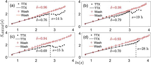
The scale-invariance for the averaged bioluminescence traces of each whole SCN slice individually are shown during-TTX and washout conditions, respectively, in Figure 2. We observe that the scale-invariance exists in the entropy estimations versus duration time s for both conditions. However, a difference is observed in the scale-invariant range and slope (scaling exponent) between these two conditions. The scale-invariant scales s show different ranges in the different conditions, the ranges being from the lower limit of 2 h, 2 h, 2 h, and 2 h to upper limit of 14 h, 19 h, 15 h, and 28 h in the TTX condition, and from 2 h, 2 h, 2 h, and 2 h to 35 h, 47 h, 48 h, and 57 h in the washout-condition, for the four slices, respectively. Accordingly, the upper limit of the range is significantly (p = .002, paired t-test) larger for the washout condition (47 h ± 9 h; mean ± SD) than for the TTX condition (19 h ± 6 h; mean ± SD). The scaling exponent (slope) is 0.76, 0.79, 0.69, and 0.70 for the TTX condition, and for 0.96, 0.98, 0.94, and 0.93 for the washout condition, within each slice, respectively. The scaling exponent is significantly (p < .001, paired t-test) larger for the washout condition (0.95 ± 0.02; mean ± SD) than for TTX (0.74 ± 0.04; mean ± SD), and as such much closer to 1.

Figure 2. The scale-invariant behaviors for each SCN slice calculated from the averaged whole SCN bioluminescence trace in the stage of TTX or washout. (a) Slice 1. (b) Slice 2. (c) Slice 3. (d) Slice 4. $\mathbf{l}\mathbf{n}\left(s\right)$ is the logarithmic value of window size $s$, and $S_{cBEDE}\left(s\right)$ is the entropy which is calculated from the averaged bioluminescence reporter data of each whole SCN slice by the cBEDE method. The parameter $\delta$ represents the slope (scaling exponent). The dashed lines indicate the upper limit of the scale-invariant range for the stage of TTX

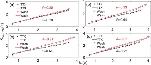
Next, the scale-invariant behaviors for every neuron in a slice were averaged over all neurons within that slice. These average scale-invariant slopes are shown during TTX application and washout, respectively in Figure 3. We observe that the scale-invariance exists in the entropy estimations versus duration time s for both the TTX and washout conditions. However, the difference is observed in the scale-invariant range and the scaling exponent between these two conditions. The scale-invariant range s is from 2 h, 2 h, 2 h, and 2 h to 35 h, 35 h, 35 h, and 33 h for the TTX condition, and from 2 h, 2 h, 2 h, and 2 h to 35 h, 47 h, 48 h, and 57 h for the washout condition, for these four slices, respectively. Accordingly, the upper limit of the scale-invariant range is significantly larger (p = .04, paired t-test) for washout (35 h ± 1 h) compared to TTX (47 h ± 9 h). The scaling exponent (slope) is 0.70, 0.64, 0.64, and 0.72 in the TTX condition, and for the washout condition it is 0.80, 0.93, 0.91, and 0.87, for these four slices, respectively. The scaling exponent is significantly (p = .02, paired t-test) larger for washout (0.88 ± 0.05; mean±SD) than TTX (0.68 ± 0.04; mean ± SD), and also much closer to 1.

Figure 3. The averaged scale-invariant behaviors taken from every individual neuron in a SCN slice in the state of TTX or washout. (a) Slice 1. (b) Slice 2. (3) Slice 3 (d) Slice 4. $\mathbf{l}\mathbf{n}\left(s\right)$ is the logarithmic value of window size $s$, and $S_{cBEDE}\left(s\right)$ is the averaged entropy of all neurons within each SCN slice by the method of cBEDE. The parameter $\delta$ represents the slope (scaling exponent)

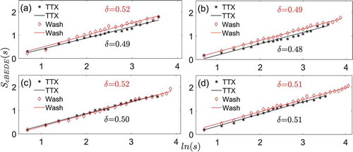
Figure 4 is the counterpart of Figure 2 for the randomized shuffled data. It is evident that the scale-invariance maintains across the investigated scales, and the scaling exponent is around 0.5 for both the TTX and washout conditions. The scaling exponents are not significantly different (p = .10, paired t-test) between the TTX (0.51 ± 0.01; mean ± SD) and the washout condition (0.50 ± 0.01; mean ± SD). As the data are randomized, the slopes are also close to 0.5, which indeed indicates uncorrelated randomness in these shuffled time series.

Figure 4. The scale-invariant behaviors for each SCN slice calculated from the averaged whole SCN bioluminescence trace based on the shuffled data. (a) Slice 1. (b) Slice 2. (c) Slice 3. (d) Slice 4. $\mathbf{l}\mathbf{n}\left(s\right)$ is the logarithmic value of window size $s$, and $S_{cBEDE}\left(s\right)$ is the entropy which is calculated from the mean of shuffled bioluminescence reporter data from all cells within each SCN slice by the method of cBEDE. The parameter δ represents the slope (scaling exponent). This figure corresponds to Figure 2

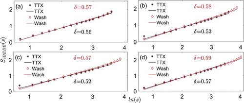
Figure 5 shows the same type of information as Figure 3, but for the shuffled data. It is evident that the scale-invariance maintains across the investigated scales, and the scaling exponent is around 0.5 for both the TTX and washout conditions. The scaling exponents are not significantly (p = .06, paired t-test) different between the TTX (0.55 ± 0.02; mean ± SD) and the washout condition (0.58 ± 0.01; mean ± SD), again close to 0.5.

Figure 5. The averaged scale-invariant behaviors taken from every individual neuron in a SCN slice based on the shuffled data. (a) Slice 1. (b) Slice 2. (c) Slice 3. (d) Slice 4. $\mathbf{l}\mathbf{n}\left(s\right)$ is the logarithmic value of window size $\mathbf{s}$, and $S_{cBEDE}\left(s\right)$ is the averaged entropy of shuffled data from individual neurons within each SCN slice by the method of cBEDE. The parameter δ represents the slope (scaling exponent)

Conclusions and discussions

In the present study, the scale-invariant behaviors of single neurons were examined during the application of TTX, indicating a decline of the network connectivity in the brain slice, and after the washout of TTX, indicating a condition where the network was restored. We used an entropy approach on the bioluminescence traces of these neurons. We found that the scale-invariant behaviors significantly differ in individual neurons as well as in the SCN slice as a whole between the conditions of reduced network connectivity (TTX) and restored network connectivity (washout). In particular, the upper time limit, which is the bin size, where the scale-invariant range is still present is significantly larger in the washout condition (47 h ± 9 h, mean ± SD for individual neurons; 47 h ± 9 h, mean ± SD for SCN slice) than during TTX application (35 h ± 1 h, mean ± SD for individual neurons; 19 h ± 6 h, mean ± SD for SCN slice), and the scaling-exponents are also significantly closer to 1 in the washout condition (0.88 ± 0.05, mean ± SD for individual neurons; 0.95 ± 0.02, mean ± S D for SCN slice) compared to the TTX condition (0.68 ± 0.04, mean ± SD for individual neurons; 0.74 ± 0.04, mean ± SD for SCN slice). For comparison, the scaling exponents do not differ significantly between the randomized shuffled data of these two conditions, both being close to 0.5, which is indicative of complete randomness in the data. This shows that our results found in the actual data are not coincidental.

In a previous study (Hu et al. 2012), the scale-invariant range of the SCN network was found to range from minutes to 10 h in multi-unit activity data, based on the DFA method. This restriction of 10 h was due to the restricted length of the data time series and the use of the DFA method. In the present study, time series of bioluminescence were used that contained much fewer data-points per 24 h than the time series used in previous studies, but the recordings lasted for more days. Due to the restricted number of data points in these time series, the cBEDE method was used, which is tailored for use in short time series. This new method enables us to examine the scale invariance at real circadian time scales, being days. The upper limit of the scales is 46.8 h, almost two daily cycles of 24 h, which is evidently longer than 10 h. The upper limit of 46.8 h suggests that the SCN controls scale-invariant behaviors even at the scale of about 2 d. Note that, because the interval of concurrent data points in the time series (bins) is 1 h for the present data, it was obviously not possible to examine time ranges of less than 2 h, which is longer than minutes in the previous studies. The difference in both the scaling-invariant range and the scaling exponents between the current and previous study may be due to differences in the data as well as methods to determine the scale-invariance.

Experimental studies have found that the application of TTX leads to decoupling between the SCN neurons, and the washout of TTX restores coupling between the neurons (Abel et al. 2016). As the scaling-exponent in the washout condition is much closer to 1 than in the TTX condition, we show that the neuronal coupling is essential for scale invariant behavior in both the individual neurons and the SCN network. In the TTX condition, the scaling exponent is much closer to 0.5, indicating more randomness in the network. However, the scaling-exponent in the TTX condition is still slightly larger than 0.5 for the corresponding randomized shuffled data, which suggests that the coupling is not completely lost after the application of TTX. Our interpretation of these results is that the value of the scaling-exponent may be indicative of the strength of the coupling in the SCN network, which means that the coupling is reduced in the TTX condition compared to the washout condition, but not completely abolished. The reduced coupling strength leads to a circadian system that may not be able to maintain a stable rhythm when challenged even by mild external disturbances. The system reacts too fast to each external influence, because the optimal balance between flexibility and rigidity is nudged toward too much flexibility.

As shown in Figure 1, after the application of the TTX, not only the cellular coupling but also the amplitudes of the individual neurons are reduced. Thus, the alternation of the scale-invariance may not only result from reduction of coupling strength but also reduction of amplitudes after the application of the TTX. In future, it will be worthwhile to identify whether the amplitude, the cellular coupling, or both determine the scale-invariance behaviors.

The scaling-exponent of ~0.6 suggests that there is a weaker positive correlation in the entropy in the TTX condition, and the scaling-exponent of ~1.0 suggests that a stronger positive correlation exists in the entropy for the washout condition. Interestingly, the scaling exponent of ~0.5 suggests that no correlation exists for the shuffled data. Therefore, it implies that the positive correlations for the original data result from the temporal patterns of organization in the data that stem from the emergent network properties, and that the actual values of the recorded data do not matter that much. The application of a scale-invariance measure on the data of single SCN neurons confirms the importance of the network in the SCN, but also that cBEDE can be a good tool to investigate the state of the SCN network, as this is reflected in the temporal patterns in the data.

Additional information

Funding

This work is supported by the National Natural Science Foundation of China under Grant Nos. 11875042 (C.-G. Gu), 11505114 (C.-G. Gu), and 11805128 (T.-F. Weng), the Natural Science Foundation of Guangxi Zhuang Autonomous Region under Grant No. 2019GXNSFAA185063 (C.-G. Gu), and the Shanghai project for construction of top disciplines under Grant No. USST-SYS-01 (H.-J. Yang, C.-G. G, and T.-F. Weng).

References

- Abel JH, Meeker K, Granados-Fuentes D, John PCS, Wang TJ, Bales BB, Doyle FJ, Herzog ED, Petzold LR. 2016. Functional network inference of the suprachiasmatic nucleus. PNAS. 113(16):4512–4517.doi:10.1073/pnas.1521178113
- Carbone A, Castelli G, Stanley HE. 2004. Time-dependent hurst exponent in financial time series. Physica A. 344(1–2):267–271.doi:10.1016/j.physa.2004.06.130
- Feng W, Yang Y, Yuan Q, Gu C, Yang H. 2019. Evolution of scaling behaviors in currency exchange rate series. Fractals. 27(02):1950005. doi:10.1142/S0218348X19500051
- Grigolini P, Palatella L, Raffaelli G. 2001. Asymmetric anomalous diffusion: an efficient way to detect memory in time series. Fractals. 9(04):439–449.doi:10.1142/S0218348X01000865
- Gu C, Coomans CP, Hu K, Scheer FA, Stanley HE, Meijer JH. 2015. Lack of exercise leads to significant and reversible loss of scale invariance in both aged and young mice. PNAS. 112(8):2320–2324.doi:10.1073/pnas.1424706112
- Gu C, Wang P, Weng T, Yang H, Rohling J. 2019. Heterogeneity of neuronal properties determines the collective behavior of the neurons in the suprachiasmatic nucleus. MBE. 16(4):1893–1913.doi:10.3934/mbe.2019092
- Hu K, Meijer JH, Shea SA, Tjebbe Vander Leest H, Pittman-Polletta B, Houben T, van Oosterhout F, Deboer T, Scheer FA. 2012. Fractal patterns of neural activity exist within the suprachiasmatic nucleus and require extrinsic network interactions. PLoS One. 7(11):e48927.doi:10.1371/journal.pone.0048927
- Hu K, Scheer FA, Ivanov PC, Buijs RM, Shea SA. 2007. The suprachiasmatic nucleus functions beyond circadian rhythm generation. Neuroscience. 149(3):508–517. doi:10.1016/j.neuroscience.2007.03.058
- Hu K, Van Someren EJ, Shea SA, Scheer FA. 2009. Reduction of scale invariance of activity fluctuations with aging and alzheimer’s disease: involvement of the circadian pacemaker. PNAS. 106(8):2490–2494. doi:10.1073/pnas.0806087106
- Li M 2010. Fractal time series—a tutorial review. Mathematical Problems in Engineering. doi:10.1155/2010/157264
- Li M, Li J-Y. 2017. Generalized cauchy model of sea level fluctuations with long-range dependence. Physica A. 484:309–335. doi:10.1016/j.physa.2017.04.130
- Mäkikallio TH, Høiber S, Køber L, Torp-Pedersen C, Peng C-K, Goldberger AL, Huikuri HV, Investigators T. 1999. Fractal analysis of heart rate dynamics as a predictor of mortality in patients with depressed left ventricular function after acute myocardial infarction. Am J Cardiol. 83(6):836–839. doi:10.1016/s0002-9149(98)01076-5
- Pan X, Hou L, Stephen M, Yang H. 2014a. Long-term memories in online users’ selecting activities. Phys Lett A. 378(35):2591–2596.doi:10.1016/j.physa.2005.02.076
- Pan X, Hou L, Stephen M, Yang H, Zhu C. 2014b. Evaluation of scaling invariance embedded in short time series. PloS One. 9(12):e116128. doi:10.1371/journal.pone.0116128
- Qi J, Yang H. 2011. Hurst exponents for short time series. Phy Rev E. 84(6):066114. doi:10.1103/PhysRevE.84.066114
- Ren H, Yang Y, Gu C, Weng T, Yang H. 2018. A patient suffering from neurodegenerative disease may have a strengthened fractal gait rhythm. IEEE Trans Neural Syst Rehabil Eng. 26(9):1765–1772. doi:10.1109/TNSRE.2018.2860971
- Roulston MS. 1999. Estimating the errors on measured entropy and mutual information. Physica D. 125(3–4):285–294. doi:10.1016/S0167-2789(98)00269-3
- Scafetta N, Grigolini P. 2002. Scaling detection in time series: diffusion entropy analysis. Phy Rev E. 66(3):036130. doi:10.1103/PhysRevE.66.036130
- Vansteensel MJ, Michel S, Meijer JH. 2008. Organization of cell and tissue circadian pacemakers: A comparison among species. Brain Res Rev. 58(1):18–47. doi:10.1016/j.brainresrev.2007.10.009
- Welsh DK, Takahashi JS, Kay SA. 2010. Suprachiasmatic nucleus: cell autonomy and network properties. Annu Rev Physiol. 72:551–577. doi:10.1146/annurev-physiol-021909-135919
- Xiong W, Faes L, Ivanov PC. 2017. Entropy measures, entropy estimators, and their performance in quantifying complex dynamics: effects of artifacts, nonstationarity, and long-range correlations. Phy Rev E. 95(6):062114. doi:10.1103/PhysRevE.95.062114
- Zhang W, Qiu L, Xiao Q, Yang H, Zhang Q, Wang J. 2012. Evaluation of scale invariance in physiological signals by means of balanced estimation of diffusion entropy. Phy Rev E. 86(5):056107. doi:10.1103/PhysRevE.86.056107