A stochastic recurrence equations approach for score driven correlation models

ABSTRACT

We describe stationarity and ergodicity (SE) regions for a recently proposed class of score driven dynamic correlation models. These models have important applications in empirical work. The regions are derived from sufficiency conditions in Bougerol (1993) and take a nonstandard form. We show that the nonstandard shape of the sufficiency regions cannot be avoided by reparameterizing the model or by rescaling the score steps in the transition equation for the correlation parameter. This makes the result markedly different from the volatility case. Observationally equivalent decompositions of the stochastic recurrence equation yield regions with different shapes and sizes. We use these results to establish the consistency and asymptotic normality of the maximum likelihood estimator. We illustrate our results with an analysis of time-varying correlations between U.K. and Greek equity indices. We find that also in empirical applications different decompositions can give rise to different conclusions regarding the stability of the estimated model.

KEYWORDS:

• Asymptotic normality
• consistency
• dynamic copulas
• generalized autoregressive score models
• observation driven models
• stochastic recurrence equations

JEL CLASSIFICATION:

• C22
• C32
• C58

1. Introduction

Time-variation in correlations is an important feature of economic and financial data and a crucial ingredient of empirical analyses, such as the assessment of risk and the construction of investment portfolios. Available models for capturing the time-variation in correlations include, amongst many others, the Baba-Engle-Kraft-Kroner (BEKK) model of Engle and Kroner (1995), the switching correlation models of Pelletier (2006), the dynamic conditional correlation (DCC) model of Engle (2002) with its adaptation by Aielli (2013), the dynamic equicorrelation (DECO) model of Engle and Kelly (2012), the dynamic copula models of Patton (2009) and Oh and Patton (2012), and the score driven models of Creal et al. (2011, 2013) and Harvey (2013); see also the overviews of Bauwens et al. (2006) and Silvennoinen and Teräsvirta (2009).

We focus on the stochastic properties of the recently proposed score driven models of Creal et al. (2011, 2013) and Harvey (2013), which we refer to as generalized autoregressive score (GAS) models. These models have proved particularly useful when modeling fat-tailed or skewed data, such as often encountered in empirical finance; see for example Janus et al. (2014), Harvey and Luati (2014), and Lucas et al. (2014). The dynamics of correlations and volatilities in these models are driven by the score of the predictive conditional distribution. If the latter is fat-tailed, the score driven dynamics automatically correct for influential observations, see Creal et al. (2011). In this way, they share some similarities with models from the robust generalized autoregressive conditional heteroskedasticity (GARCH) literature; see for example Boudt et al. (2013). The score driven approach used in the construction of GAS models, however, provides a much more general and unified framework for parameter dynamics that is applicable far beyond the volatility and correlation context; see Creal et al. (2013, 2014) for a range of other examples. In addition, from a forecasting perspective GAS models often have a similar performance to correctly specified state-space models, see Koopman et al. (2012).

Despite their proven empirical usefulness, the theoretical properties of GAS models are less well developed. The complication lies in the highly nonlinear transition dynamics of the time-varying parameter in typical GAS models. In this article, we contribute to our understanding of the stochastic properties of GAS models for dynamic correlations. The fundamental question is to understand which parameterizations, and parameter values generate stationary and ergodic (abbreviated as SE from now on) time series processes. This offers an important characterization of the stochastic properties of GAS models. SE properties can be combined with the existence of unconditional moments for the objective function to establish proofs of consistency and asymptotic normality of extremum estimators; see, e.g., Straumann and Mikosch (2006) for maximum likelihood estimation of nonlinear conditional volatility models, Francq and Zakoian (2011) and Boussama et al. (2011) for the case of multivariate GARCH models, and Harvey (2013) for GAS volatility models. For each correlation model we consider, we identify the parameter values that ensure the SE property and call this the “SE region” of the parameter space. To establish SE regions, we follow the classical average contraction argument for stochastic recurrence relations as laid out in the sufficient conditions formulated by Bougerol (1993). Given these conditions, we compute numerically the SE regions for a range of empirically relevant models.

We have four contributions. First, we are the first to derive SE regions for the class of score driven correlation models that have been suggested recently in the literature. We show that the SE sufficiency regions take a highly nonstandard form, dissimilar to the familiar triangle and curved triangular shapes for the GARCH model; see Nelson (1990). In an empirical example, we demonstrate that the conditions for nonlinear recurrence equations can be used to ensure stationarity of concrete models, applied on real data. This also extends the results in Blasques et al. (2014b) for volatility and tail index models with univariate observations to the case of time-varying parameters and multivariate observations.

Second, we show that the shape and size of the SE sufficiency region as derived from the conditions of Bougerol (1993) depends on the way the stochastic recurrence equation for the correlation is constructed from bivariate uncorrelated noise. In particular, we show that the choice of the square root of the correlation matrix in this construction has a nontrivial effect on the size of the SE sufficiency region.

Third, we show analytically why the correlation case is markedly different from the volatility case. For the volatility case, Harvey (2013) shows that modeling the log-volatility renders the information matrix independent of the time-varying volatility. The resulting stochastic recurrence equation becomes linear, and we can use linear process theory to study the SE properties. A similar feature is generally not available for the dynamic correlation model: neither a reparameterization of the correlation nor a scaling of the score steps makes the stochastic recurrence equation a linear process. The reason is that unlike in the volatility case, the GAS steps for the correlation model consist of two separate terms with different nonlinearities in the correlation parameter.

Fourth, we use our SE results to establish the consistency and asymptotic normality of the ML estimator.

The remainder of this article is organized as follows. In Section 2, we introduce our model for dynamic bivariate correlations. In Section 3, we state the conditions for the SE sufficiency regions. In Section 4, we establish model invertibility as well as the consistency and asymptotic normality of the ML estimator. In Section 5, we determine the SE regions numerically for a number of different models and provide an empirical illustration for U.K. and Greek equity indices. We conclude in Section 6. The Appendix gathers the more technical results and derivations.

2. Score models for correlations

Consider a real-valued bivariate stochastic sequence of observations {y_t}_t∈ℕ generated by a zero mean elliptical conditional distribution with time-varying correlation matrix R(f_t)

(1)

where denotes a real-valued density generator function in the quadratic form , the sequence {f_t}_t∈ℕ is a real-valued sequence for the time-varying parameter f_t, ρ(f_t) ∈ [ − δ, δ] with δ ∈ (0, 1] is the dynamic correlation parameter at time t, and R(f_t) is the correlation matrix at time t. For example, if y_t is conditionally normal, we have p(x) = (2π)⁻¹exp (−x/2). We fully focus the exposition on the correlation case by restricting the variances in (1) to one. Time-varying variances in score driven models have already been dealt with in for example Creal et al. (2011) and Harvey (2013).

The formulation in (1) can also be interpreted as a copula model, see the discussion in Patton (2009). Under the assumptions of stationary marginals and no volatility spillovers, stability conditions for the copula then lead to stability of the whole model. The class of elliptical models is also economically interesting, as it enables an analytic characterization of the resulting portfolio returns and the risk-return trade-off; see for example Chamberlain (1983), Owen and Rabinovitch (1983), and Hamada and Valdez (2008).

Following Creal et al. (2011, 2013), the GAS dynamics for the time-varying parameter f_t in (1) take the form

(2)

(3)

with an arbitrary fixed initial condition f₁ ∈ ℱ. We define the parameter vector θ ∈ Θ as θ = (ω, α, β, λ), where (ω, α, β) ∈ ℝ³ is a vector of updating parameters, and λ ∈ ℝ^n_λ allows n_λ ≥ 0 density tail shape parameters to be estimated. The time-invariant parameter space is described by Θ ⊆ ℝ^3+n_λ. We suppress dependence of the scaling and the score on θ by writing s(f_t, y_t) ≡ (f_t, y_t; λ), S(f_t) ≡ S(f_t; λ), and q(y_t, f_t) ≡ q(y_t, f_t; λ). For the case of the bivariate correlation model (1), we obtain

(4)

with ṗ(x) = ∂log p(x)/∂x and .

Each choice for the scaling function S in (3) gives rise to a new GAS model. An often used choice of S relates to the local curvature of the score as measured by the information matrix, for example

(5)

where a is typically taken as 0, 1/2 or 1.

The parameter dynamics in (2) and (3) are intuitive. The time-varying parameter f_t is updated in the (scaled) direction of steepest ascent as measured by the scaled conditional log observation density at time t. For example, standard GARCH and BEKK models are special cases of the GAS framework under normality, see Creal et al. (2013). The GAS setup is very general and can also easily be applied outside the correlation context as long as a conditional observation density is available. For other examples, including many new models, we again refer to Creal et al. (2013, 2014).

3. Conditions for stationarity and ergodicity

We follow the approach of Blasques et al. (2014b), who consider a treatment of univariate GAS models. Our SE results build on the stochastic recurrence relations or iterated random functions approach; see Diaconis and Freedman (1999) and Wu and Shao (2004). In particular, we use the sufficient conditions of Bougerol (1993) and results in Straumann and Mikosch (2006) to establish, for any fixed initial condition f₁ ∈ ℱ, exponentially fast almost sure convergence of the time series {y_t, f_t(θ, f₁)}_t∈ℕ generated by (1)–(3) to a unique SE solution {y_t, f_t(θ)}_t∈ℤ.

Let ℱ ⊆ ℝ and 𝒴 ⊆ ℝ² denote the domains of f_t and y_t, respectively. We have that ρ: ℱ → (− δ, δ) for 0 < δ ≤1 and s: ℱ × 𝒴 × Θ → ℝ is almost surely (a.s.) smooth in all its arguments and Lipschitz in f ∈ ℱ. Using the model as specified in (1)–(4), we analyze the stochastic properties of y_t and f_t via the stochastic recurrence equation

(6)

and {u_t} is an independent and identically distributed (i.i.d.) sequence with y_t = h(f_t)u_t. We notice that the dynamics of {f_t} in (6) are now written in terms of the innovation sequence {u_t} rather than the observed data {y_t} by substituting h(f_t)u_t for y_t. As a result, when seen as a function of f, the shape of q(h(f)u_t, f), for every u_t, is markedly different from that of q(y_t, f), for every y_t. This additional dependence on f may either complicate or simplify the nonlinear dependence of f_t+1 on f_t as embedded in (6). Second, the functional form of (6) is not uniquely defined. Each square root h(f) of the correlation matrix R(f) leads to an observationally equivalent model in y_t. The choice of h(f), however, is not innocuous for determining the size and shape of the SE region, as we see later.

Continuity of φ_t in u_t for every t can be used to ensure that {φ_t} is an i.i.d. sequence of functions. Together with Eq. (6), it then follows directly from Bougerol (1993) and Straumann and Mikosch (2006) that there is a unique SE solution to (1)–(3) if φ_t is contracting on average, i.e., if the Lyapunov exponent of the mapping is negative. In particular, we obtain the desired SE result if

(7)

see Bougerol (1993). In computing the supremum in condition (7), f is treated as a parameter rather than as the random variable f_t.

For the score driven dynamic correlation model of Section 2, we prove the following result in the Appendix.

Lemma 1

Let Ψ be a class of functions such that for every ψ ∈ Ψ, ψ ∈ 𝒞¹([ − δ, δ], ℝ) with . Assume that for i, j ∈ {1, 2}, with u_t = (u_{1, t}, u_{2, t})^⊤. For any fixed initial condition f₁ ∈ ℱ, the process {f_t(θ, f₁)}_t∈ℕ generated by the dynamic correlation model (1)–(4) converges exponentially fast almost surely¹ (e.a.s.) to a unique stationary and ergodic solution {f_t(θ)}_t∈ℤ if

(8)

where

(9)

(10)

ġ(ρ) = ∂g(ρ)/ρ, c_2ψ(ρ) = cos (2ψ(ρ)), and s_2ψ(ρ) = sin (2ψ(ρ)).

We note several features of the result stated in Lemma 1. First, the SE region only depends directly on the parameters α and β, on the functional forms of S(f) and q(h(f)u_t, f), and on the density of u_t. The dependence on the latter enters in two ways, namely through the expectations operator in (8) and through the functional form of k(u_t) in (10). Also note that the expectations operator in (8) does not necessarily require the second moments of u_t to exist. Instead, we only require the expectation of for i, j ∈ {1, 2} to exist. This condition is much weaker, particularly for fat-tailed elliptical densities. For example, it is easily satisfied for the bivariate Cauchy distribution, even though neither the second nor the first moment exists for this distribution. The continuity and boundedness properties of s can be verified immediately for parametric distributional forms, notably for the Student's t density in Section 5.1.² Therefore, condition (8) effectively forms a sufficient condition for the SE property of the model.

Second, Eq. (8) directly reveals that the correlation case is markedly different from the volatility case. For the volatility case, it is shown in Harvey (2013) and Blasques et al. (2014b) that through a clever choice of parameterization h or scaling S the scaled score in recurrence relation (6) can be made independent of f_t. The SE condition then reduces to the requirement that |β| <1. In the volatility case the analogue of the function g(ρ) in (9) is scalar valued. In the correlation case, Eq. (8) shows that through the trivariate nature of the functions g(ρ) and ġ(ρ) the contraction condition consists of a number of different terms, each with a different nonlinear dependence on f. It is impossible to offset all of these simultaneously by a single choice of scaling function or parameterization. This makes the correlation model theoretically more interesting in its own right.

Third, the SE sufficient condition in Eq. (8) has an additional degree of flexibility provided by the choice of ψ. As follows from the proof of Lemma 1, the function ψ determines which square root h(f) is used for the correlation matrix R(f). For the purpose of guaranteeing a proper correlation matrix, define ξ(ρ) = arcsin (ρ) − ψ(ρ), and

(11)

for some constant k_ψ ∈ ℝ, such that h(f)h(f)^⊤ = R(f) for all ψ ∈ Ψ. This parametrization gives rise to familiar alternatives for matrix roots. For k_ψ = 1/2, we obtain symmetric matrix root of Lemma 2, whereas the choice k_ψ = 1 reduces to the Cholesky decomposition with y_{1, t} = u_{1, t} and . Any choice of ψ and thus of h results in an observationally equivalent model for y_t. The dynamic properties of {f_t} following from (7), however, depend on the precise ψ that is chosen. We therefore obtain a sufficient condition for SE if (7) is satisfied for some choice of ψ ∈ Ψ satisfying the conditions formulated in Lemma 1. This yields the additional infimum in condition (8). A similar complication is absent in the volatility case; compare Blasques et al. (2014b) and Harvey (2013).

Fourth, condition (8) simplifies for particular choices of parameterizations and scale functions. For example, if we use the familiar Fisher transformation ρ(f) = tanh (f_t), we have and the entire middle term in (8) vanishes. For this particular parameterization and fixing the scaling function to S(f) ≡ 1, we can even provide further analytical results relating to the optimal choice of the function ψ. Using a Jensen, triangle, and Cauchy–Schwarz inequality, we obtain a stricter sufficient condition for SE from (8) as

(12)

where ‖·‖ denotes the standard Euclidean norm. Instead of the Cauchy–Schwarz inequality, we can also use a second triangle inequality to obtain the alternative stricter sufficient condition

(13)

where <gdot >_i and k_i are the ith elements of ġ and k, respectively. Using either of the more stringent SE conditions (12) or (13), we obtain the following result.

Lemma 2

Under the assumptions stated in Lemma 1, setting ψ(ρ) = k_ψarcsin (ρ) with k_ψ = 1/2 reaches the functional lower bound for the sufficient condition stated in either Eq. (12) or (13). The condition then reduces to |β| + |α| 𝔼‖k(u_t)‖ <1 \ for condition (12) and |β| + |α| 𝔼|k₁(u_t)| <1 for condition (13), respectively, where k₁(u_t) is the first element of k(u_t). The link function becomes the symmetric matrix root

The result in Lemma 2 shows that we uniformly obtain the largest SE region for the stricter conditions (12) or (13) for the symmetric matrix root h in (6). The choice of h in setting up the dynamic Eq. (6) is thus far from innocuous and directly influences the size and shape of the SE region.

4. Asymptotic properties of ML estimator

In this section we establish the invertibility of the GAS model, as well as the consistency and asymptotic normality of the maximum likelihood estimator (MLE) for the static parameters θ.

Model invertibility is a critical element in the proof of consistency and asymptotic normality of the MLE since the filter (2) enters the likelihood function and thus must be ensured to have appropriate stochastic properties. Similarly to Straumann and Mikosch (2006), this section uses the contraction condition of Bougerol (1993) in order to ensure model invertibility and bounded moments for the filtering sequence. This is crucial for the asymptotic properties of the MLE since the initialized time-varying parameter and its derivatives enter the likelihood function and its derivatives. The following result builds on the SE nature of the data {y_t}_t∈ℤ which follows easily from the SE nature of the true time-varying parameter {f_t}_t∈ℤ established in the previous section.

Lemma 3 (Model Invertibility)

Let Θ be compact, let {y_t}_t∈ℤ generated by (1)–(3) be SE, let the scaled score s be smooth in all arguments and Lipschitz in f ∈ ℱ, and assume that there exists a nonrandom f₁ such that the following statements hold:

1. 𝔼log ⁺|S(f₁)q(f₁, y_t)| < ∞;

2. 𝔼log sup _θ∈Θsup _f*|α(Ṡ(f*)q(f*, y_t) + S(f*) (f*, y_t)) + β| <1.

Here, log ⁺x ≡ max (log x, 0) for x ∈ ℝ₊ and q(f_t, y_t) is the score expression in (4). Then the GAS recursion {f_t(θ, f₁)}_t∈ℕ defined in (2) converges e.a.s. to a unique limit SE process {f_t(θ)}_t∈ℤ that admits the representation f_t(θ) = Φ(y_t−1, y_t−2,...) for every t and some measurable function Φ.

Note that the contraction condition (ii) in Lemma 3 is different from the one studied in Lemma 1 since it refers to the filtering equation that takes the data y_t as given. By contrast, the contraction property in Lemma 1 looks at the GAS model as a data generating process, and hence defines the data y_t in terms of the true unknown parameter f_t and the innovations u_t. The invertibility condition above is in particular required in order to make dependence on the fixed initial value f₁ vanish in the GAS recursion and therefore in the objective function. To make this transparent, let ℓ_t(θ, f₁) denote the time t log-likelihood contribution for the vector of static parameters θ, and

(14)

Define ℒ_T(θ) and ℓ_t(θ) similar to (14), but with the limiting process f_t(θ) replacing f_t(θ, f₁).

Theorem 1 establishes the strong consistency of the MLE assuming the identification of the true parameter vector θ₀ ∈ Θ. The strong consistency result holds for every initialization of the filter satisfying the conditions of Lemma 3.

Theorem 1 (Consistency)

Let (Θ, 𝔅(Θ)) be a compact measurable space, and let the conditions of Lemmas 1 and 3 hold. Furthermore, assume that 𝔼sup _θ∈Θ|ℓ_t(θ)| < ∞ and that θ₀ ∈ Θ is the unique maximizer of ℒ_∞(θ) ≡ 𝔼ℓ_t(θ). Then, for every f₁ ∈ ℱ, the MLE, defined as satisfies as T → ∞.

Theorem 2 establishes the asymptotic normality of the MLE. In this theorem, we let denote the Fisher information matrix and is the expected outer product of gradients, with and denoting first and second order derivatives of ℓ_t(θ) with respect to θ, respectively.

Theorem 2 (Asymptotic Normality)

Let the conditions of Theorem 1 hold, and let θ₀ be a point in the interior of Θ. Furthermore, let the first and second derivatives of the log likelihood contributions ℓ_t(θ) be asymptotically SE and satisfy and . Then, for every f₁ ∈ ℱ, the ML estimator satisfies

The theoretical results in the previous two theorems are supported by unreported simulation experiments. We find that increasing the sample size brings the ML estimates over repeated Monte Carlo replications closer to their true values in a controlled setting. Moreover, we also find that the distribution of the estimator approaches the normal distribution for increasing sample sizes.

Theorems 1 and 2 rely on high-level conditions and are applicable to the generic setting. For particular models, however, the statements can be further particularized into more transparent low-level conditions. Corollaries 1 and 2 provide such primitive conditions for the consistency and asymptotic normality of the MLE for the parameters of two bivariate models based on the normal and Student's t distribution, respectively. We use unit scaling and a parameterization given by ρ_t = δ·tanh (f_t). This automatically bounds the correlation to the interval (− δ, δ) to render the correlation matrix positive definite. The practitioner can choose a value of δ arbitrarily close to unity to obtain the contraction conditions in Lemmas 1–3. Proofs of these corollaries can be found in Section D of the Supplementary Appendix.

Corollary 1

There exists a compact parameter space Θ satisfying 0 < δ <1 and α ≠ 0, where the MLE for the parameters of the bivariate Gaussian model with δ·tanh link function and unit scaling is consistent and asymptotically normal.

Corollary 2

There exists a compact parameter space Θ satisfying 0 < δ <1, α ≠ 0, and 2 < ν, where the MLE for the parameters of the bivariate Student's t model with δ·tanh link function and unit scaling is consistent and asymptotically normal.

The implied parameter space Θ, constrained by the above conditions, depends not only on α and β, but also on distributional and parametrization choices. The shapes and sizes of the contraction regions are further analyzed in Section 5. Further analytical and numerical details are developed in Sections C and D in the Supplemental Appendix.

5. Numerical and empirical results

5.1. Numerical results

Alternative choices for the error density generator p, the scaling function S, the parameterization ρ, and the matrix square root h give rise to different models with different SE regions. For a number of these choices, we check for every pair (α, β) whether the sufficient condition (8) is satisfied. We plot the SE region in the (α, β)-plane by numerically identifying, for every fixed β, the corresponding maximum and minimum values of α that satisfy (8).

To fix ideas, consider the class of Student's t densities for u_t as in Creal et al. (2011). The Fisher transformation ρ(f_t) = tanh (f_t) ensures proper value for the correlation parameter. As indicated in Section 3, this also simplifies the evaluation of the SE condition in Lemma 1. For the scaling function S, we adopt the three choices based on the information matrix as presented in Eq. (5).

Next, we investigate the sensitivity of the SE region to the choice of matrix root h(·). For this, we consider two prominent alternatives, both described by ψ(ρ) = k_ψarcsin (ρ) for k_ψ ∈ ℝ. The first alternative is the symmetric matrix root of Lemma 2 with k_ψ = 1/2. The second is the familiar (lower triangular) Cholesky decomposition, which is obtained by setting k_ψ = 1.

To numerically evaluate the sufficient SE condition (8), we need to solve an optimization problem within an integration procedure. As the state equation is univariate, the integral can be evaluated via a quadrature rule. We can gain further numerical efficiency for the inner optimization problem by storing maximum and minimum values of S(f) q(h(f)u_t, f) for each point u_t and recycling these for evaluation at different points in the (α, β)-plane. Local optima are avoided by evaluating the function over a wide grid and by noting that for the Student's t distribution (∂/∂f)ⁱs(f, y_t) → 0 as |f| → ∞ for all i > 1. We can further halve the computation time by noting that in our setting |∂φ_t(f; θ)/∂f| = |∂φ_t(f; − θ)/∂f|.

In panel (a) of Fig. 1, we present the results for the normal distribution and the symmetric root h(f), i.e., k_ψ = 1/2. The figure contains three different regions, each one corresponding to a different form of scaling in Eq. (5). Points inside each region are combinations of (α, β) for which the sufficient condition (8) is met. The shape of the sufficient SE region is antisymmetric around the origin due to the absolute signs in (8), such that we only plot its upper half. The region also shows a nonmonotonic curvature, particularly in the second quadrant. This feature is due to the use of absolute values, the change in the location of the supremum in (8) in the second quadrant, and a shift in the relevant region of integration if the derivative of S(f)q(h(f)u_t, f) changes sign.

Figure 1 Stationarity and ergodicity sufficiency regions for the normal distribution and different scaling choices S(f) = (ℐ_t(f))^−a for a ∈ {0, 1/2, 1}. The two panels contain different regions obtained by parameterizing the matrix roots h(f) with ψ(ρ) = k_ψarcsin (ρ). Panel (a) contains the results for the symmetric matrix root (k_ψ = 1/2), and panel (b) corresponds to the Cholesky decomposition (k_ψ = 1).

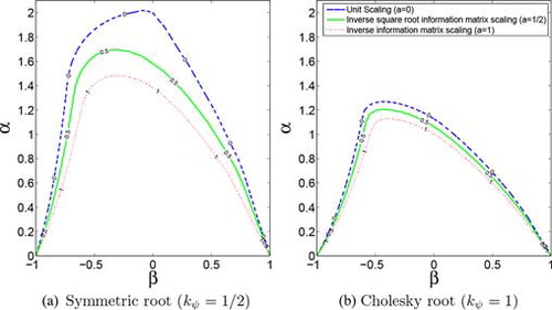
An interesting feature in Fig. 1 is the behavior of the region for square root inverse information matrix scaling, a = 1/2 in (5). First note that a = 1/2 has the property that the update via s(f_t, y_t) is invariant with respect to reparametrizations of f_t. Furthermore, under correct specification the steps S(f)q(y_t, f) in (4) are by construction martingale differences with unit variance; see also Creal et al. (2013). This implies that {f_t}_t∈ℕ converges to a covariance stationary process as long as |β| <1. The region in Fig. 1 shows that |β| <1 is necessary, but not sufficient for (8) to be satisfied. This relates directly to discussions in the GARCH literature, where in the univariate setting covariance stationarity is a more restrictive condition than strict stationarity, but the relation between the two remains an open question in a multivariate context; see for example Boussama et al. (2011).

Panel (b) in Fig. 1 shows the different SE regions for a different choice of matrix root h(f), namely the Cholesky decomposition. It is clear that the sufficiency regions in the (α, β)-plane are smaller than the corresponding regions for the symmetric root. As models constructed with a symmetric root and a Cholesky root are observationally equivalent, we can take the larger regions as sufficient regions for SE to hold; see also Lemma 2. The differences make clear that the choice of matrix root is important for determining the size of the region either analytically or numerically.

We provide more SE regions in the Supplemental Appendix, including regions based on the further inequalities used to establish Lemma 2. In particular, we show that the SE regions for the Student's t distribution under square root information matrix scaling (a = 1/2) are smaller for fatter tails if the Cholesky decomposition is used (k_ψ = 1), while the converse holds if we use the symmetric root decomposition (k_ψ = 1/2). In Section 5.2, we document how this wedge may also become empirically relevant.

5.2. Empirical illustration

In this section, we study the time-varying correlation between the London and Athens stock exchange indexes. We take daily returns of the Financial Times Stock Exchange (FTSE) 100 and the Athex Composite over the period January 1, 2002 to March 2, 2013. We are particularly interested in whether there are indications that the correlation between these two markets changed over the course of the European sovereign debt crisis.

To focus on the correlation part of the model, we first filter both series using AR-GARCH type models; see also Patton (2009). The mean of both series is modeled by a first order autoregressive progress. We find a strong leverage effects in both series and capture these by a GJR(1,2) model of Glosten et al. (1993) for the FTSE index, and an EGARCH(1,2) specification of Nelson (1991) for the Athens index, respectively.³ We test the null hypothesis of constant and zero residual correlation against time-varying alternatives using a Nyblom test of the form

where B(z) and B_b(z) = B(z) − zB(1) denote a standard Brownian motion and a standard Brownian bridge, respectively. The average correlation is estimated by and is a heteroskedasticity and autocorrelation consistent estimator of the long-run variance of , with defined similarly when is set to 0.⁴ By letting x_t denote the univariate volatility-filtered series, i.e., x_t: = y_t in the notation of our article, we find strong evidence for time-varying correlations. We therefore use the filtered univariate series to estimate the GAS model from Section 2 with a time varying correlation coefficient. The Nyblom test can further be used as a diagnostic tool for remaining time-variation in dynamic correlations when applied to estimated residuals . The results are shown in Fig. 2 and Table 1.

Figure 2 Empirical results. Panel (a) shows 60-day rolling correlations and the filtered correlations between the FTSE 100 (U.K.) and Athex Composite (Greece) equity index returns. The right panel puts the empirical estimates obtained by unconstrained estimation into the zoomed stationarity and ergodicity region perspective.

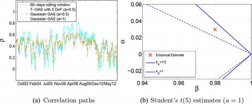
Table 1 Estimation results.

	EWMA	EWMA	EWMA	t(∞)-GAS	t(∞)-GAS	t(∞)-GAS	t(5)-GAS	t(5)-GAS	t(5)-GAS	t(λ)-GAS
				(a = 0)	(a = 1/2)	(a = 1)	(a = 0)	(a = 1/2)	(a = 1)	(a = 1)
λ	5	5	8.9321	∞	∞	∞	5	5	5	9.1411
			(0.0801)							(0.9287)
ω		0.0003	0.0012	0.0117	0.0115	0.0112	0.0089	0.0089	0.0088	0.0114
		(0.0003)	(0.0003)	(0.0016)	(0.0014)	(0.0013)	(0.0011)	(0.0011)	(0.0010)	(0.0013)
α				0.0254	0.0283	0.0314	0.0335	0.0316	0.0297	0.0360
				(0.0040)	(0.0045)	(0.0050)	(0.0048)	(0.0046)	(0.0043)	(0.0050)
β	0.9757	0.9756	0.9739	0.9752	0.9757	0.9763	0.9797	0.9798	0.9800	0.9762
	(0.0085)	(0.0063)	(0.0030)	(0.0021)	(0.0016)	(0.0012)	(0.0013)	(0.0011)	(0.0009)	(0.0012)
Log-likelihood	−7, 847	−7, 847	−7, 812	−7, 891	−7, 890	−7, 890	−7, 845	−7, 845	−7, 845	-7,809
AIC	15, 697	15, 699	15, 631	15, 778	15, 787	15, 787	15, 696	15, 696	15, 696	15,626
BIC	15, 703	15, 711	15,649	15, 814	15, 805	15, 805	15, 714	15, 714	15, 714	15,649
# parameters	1	2	3	3	3	3	3	3	3	4
H: ρt ≡ 0	reject	reject					reject	reject	reject
[3pt] H:		reject	reject	reject	reject	reject	reject	reject	reject
Inside SE region?
Cholesky (kψ = 1)				Yes	Yes	No	No	No	No	No
Symmetric ()				Yes	Yes	Yes	Yes	Yes	Yes	Yes

Heteroskedasticity and autocorrelation consistent (HAC) standard errors in parentheses. Best log-likelihood, AIC, and BIC values across models are printed in boldface. H: ρ_t ≡ 0 and H: indicate whether the Nyblom test among residuals rejects constant zero or estimated correlation, respectively. HAC standard errors are computed using Newey–West weights with min(⌊1.2 × T^1/3⌋, T) lags.

Panel (a) in Fig. 2 shows the dynamic correlations between the filtered series. As a nonparametric benchmark, we plot simple 60-day rolling window correlations. The rolling window estimates suggest that correlations exhibit clear signs of time variation. Correlations lie around 0.4 up to about 2006, then increase to about 0.6, and come down substantially to around 0.2 during the sovereign debt crisis. On top of this slow variation, there are also substantial dynamic patters at higher frequencies.

The possibly lower correlations between the U.K. and Greek stock indices are interesting economically, particularly given the stable correlation pattern between the two series during almost the whole of the prelude, height, and aftermath of the preceding financial crisis (2007–2009). The financial crisis, apparently, did not substantially alter the real economic linkages between the two economies as evidenced by the stable dynamic of the correlations between between the two stock markets. It is only after the announcement of the record Greek deficit late 2009 and the subsequent actions that gave rise to the European sovereign debt crisis, that the link between the euro-denominated Greek stock market and the sterling-denominated FTSE is broken. The correlations remain at low levels even after the nonstandard monetary policy actions by the European Central Bank.

Table 1 provides the parameter estimates of the GAS models. We provide a benchmark by estimating a simple exponentially weighted moving average (EWMA) scheme for the correlation based on the recursion ρ_t = tanh (f_t) and

see also the Gaussian dynamic copula specification of Patton (2006).

We see that the GAS model is empirically useful both in terms of in-sample likelihood fit and improving the diagnostics for time-varying correlation. All models indicate that the correlation parameter is highly persistent: the estimated values of β all lie very close to 1. The scaling function for the score only has a mild effect on the model's fit: the likelihood values are similar for a = 0, 1/2, 1. The degrees of freedom parameter λ is estimated around 9. This is substantially fatter-tailed than the normal, but also substantially lighter-tailed than the Student's t distribution with the degrees of freedom fixed at 5. The differences in likelihood values, as well as Akaike (AIC) and Bayes (BIC) information criteria indicate that estimating the degrees of freedom improves the fit of the model substantially. Furthermore, the estimation of the tail parameter λ also improves the fit in terms of model diagnostics: only the GAS model with estimated degrees of freedom passes the Nyblom tests for remaining time-variation in the residual cross-correlations.

We plot the SE region boundaries for the Cholesky and the symmetric root decomposition in panel (b) of Fig. 2. The estimated values of α and β for the t(λ)-GAS specification are indicated by the cross mark. The results clearly confirm the importance of the choice of ψ in verifying the SE properties. For the symmetric root-based region, we obtain stationarity and ergodicity at the estimated parameter values. For the Cholesky decomposition, by contrast, we fail to obtain this result. As condition (8) takes the infimum over ψ and thus the widest region in panel (b) over all admissible decompositions h(f_t), the Cholesky decomposition is in this setting less powerful to discriminate SE from non-SE regions of the parameter space. We stress again that all of these regions are only based on sufficient conditions, and that the actual regions may be wider.

For all models considered, the bottom lines in Table 1 indicate whether the estimated parameters lie inside the SE region. For the Gaussian models with unit (a = 0) and inverse square root information matrix scaling (a = 1/2) the choice of matrix decomposition does not have an impact. Both the symmetric root (k_ψ = 1/2 in (11)) and Cholesky root (k_ψ = 1 in (11)) indicate that the estimated parameters are inside the SE region and satisfy the average contraction condition. For inverse information matrix scaling, however, and for the Student's t based models, we find a similar difference as in panel (b) of Fig. 2: we cannot ensure SE properties based on the Cholesky decomposition, whereas we can do so for the symmetric root. This again highlights that the use of different constructive devices such as different matrix decompositions is empirically relevant for the verification of sufficient SE conditions in a multivariate setting.

6. Concluding remarks

We have derived sufficient regions for stationarity and ergodicity for a new class of score driven dynamic correlation models. The regions exhibit a highly nonstandard shape. Moreover, we have shown that the shape and size of the SE regions depends on the type of matrix root that is chosen in checking the sufficient conditions of Bougerol (1993). Furthermore, we have seen how the stationarity conditions can be used in establishing results for consistency and asymptotic normality of the maximum likelihood estimator. The numerical stability conditions were supported by an empirical investigation of the time varying correlation between U.K. and Greek stock markets. We found a substantial drop in the linkages between the sterling-denominated U.K. market and the euro denominated Greek market over the course of the European sovereign debt crisis. Such a break in dependence between markets, however, was absent during the preceding global financial crisis.

An interesting possible extension of our current results concerns a generalization to the fully multivariate (rather than bivariate) setting of score driven correlation models proposed in Creal et al. (2011). The challenge here is to limit the number of parameters describing the dynamics of time-varying volatilities and correlations. We leave this for future work.

Acknowledgments

A previous version of this article was circulated under the title “Stationarity and Ergodicity Regions for Score Driven Dynamic Correlation Models.” We thank Peter Boswijk and Andrew Harvey for helpful discussions. We also thank participants of the Amsterdam–Cambridge Conference on Score Driven Models (2013) and participants of 7th International Conference on Computational and Financial Econometrics (CFE 2013) for comments.

Notes

A sequence {x_t} converges exponentially fast almost surely to a sequence if for some constant c > 1 we have for t → ∞.

The functional forms for the updating equation for the particular case of the Student's t distribution are presented in the Supplemental Appendix accompanying this article.

Further robustness results for alternative specifications for the marginals can be found in Section E of the Supplemental Appendix.

Critical values of the test are simulated by discretizing the processes B(·) and B_b(·) and can also be found in Hansen (1992).

Appendix A: Proofs

We first state Theorem 3.1 of Bougerol (1993). Denote by log Λ(φ₀) the term inside the expectation on the left-hand side of (7).

Theorem 3 (Bougerol, 1993, Theorem 3.1)

Let {φ_t} be a stationary and ergodic sequence of endomorphic Lipschitz maps. Assume as follows:

1. There exists a f ∈ ℱ and distance measure d such that 𝔼[log ⁺d(φ₀(f), f)] < ∞;

2. 𝔼[log ⁺Λ(φ₀)] < ∞;

3. where denotes the r-fold backward iterates.

Then the stochastic recurrence Eq. (6) admits a stationary ergodic solution {f_t}.

Proof of Lemma 1

The SE property of {f_t} follows from the measurability with respect to {u_t}. The Lipschitz property is obtained from the boundedness of the terms in Eq. (A6) below. Condition 3 is then ensured by the definition of the GAS transition equation and the assumed moments in Lemma 1, as we can write 𝔼[log ⁺d(φ₀(f), f)] ≤ 𝔼|φ₀(f) − f| = 𝔼|ω + (β −1)f + αS(f)q(h(f)u₀, f)| ≤ |ω| + |(β −1)f| + α𝔼|S(f)q(h(f)u₀, f)|. As requirement 3 is implied by 3, we can now turn our main interest towards the study of the latter, nontrivial, condition 3.

We write ξ and ψ for ξ(ρ) and ψ(ρ), respectively. Define the shorthand notation c_w = c_w(ρ) = cos (w(ρ)) with w: [ − δ, δ] → ℝ, and similarly s_w = s_w(ρ) = sin (w(ρ)). Each matrix root h of the correlation matrix can be written as

(A1)

Using (A1), we obtain

such that we require sin (ψ + ξ) = ρ or ξ(ρ) = arcsin (ρ) − ψ(ρ) for some arbitrary function ψ(ρ). It follows that and From this, we obtain

Using y_t = h(f)u_t, we can rewrite (4) as

(A2)

with

and u_t = (u_{1, t}, u_{2, t})^⊤. Defining ġ(ρ) = ∂g(ρ)/ρ as the derivative of g(ρ), it holds that

(A3)

(A4)

The definitions in (6) and (A2) then imply that (7) can be written as

(A5)

Proof of Lemma 2

Using (A4), we can rewrite ‖ġ(ρ)‖² as

(A6)

For ψ(ρ) = arcsin (ρ)/2, the second term vanishes, and we obtain the functional lower bound (1 − ρ²)·‖ġ(ρ)‖² = 1 − ρ², which reaches its supremum of 1 at ρ = 0. The rest of the result follows directly from the definition of ξ(ρ) = arcsin (ρ) − ψ(ρ) = arcsin (ρ)/2. For computational reasons, it may be useful to note that

which only depends on the quadratic form .

An analogous line of reasoning holds for condition (13) based on applying the triangle inequality twice.

Proof of Lemma 3

The proof follows immediately from Theorem 2.8 in Straumann and Mikosch (2006) by noting that our conditions (i) and (ii) imply conditions S.1 and S.2 in their theorem.

Proof of Theorem 1

We follow Blasques et al. (2014a) and appeal to Theorem 3.4 of White (1994), and obtain from the uniform convergence of the criterion function and the identifiable uniqueness of the maximizer θ₀ ∈ Θ defined, e.g., in White (1994).

Existence. Note that ℒ_T(θ, f₁) is a.s. continuous in θ ∈ Θ if each likelihood contribution is. This is obtained by the smoothness of the scaled score s: ℱ × 𝒴 × Θ → ℝ and the resulting continuity of f_t in θ as a composition of t continuous maps. Due to the compactness of Θ, by Weierstraß\ theorem, the arg max set of the likelihood is nonempty a.s., and hence exists.

Uniform Convergence. By an application of the triangle inequality, we have

The first term in (A7) vanishes by the convergence of f_t(y^{1: t−1}, θ, f₁) to f_t(y^t−1, θ) which is established in Lemma 3. The maintained smoothness assumption on the scaled score ensures that ℓ_t(·, f₁) = ℓ(f_t(y^{1: t−1}, ·, f₁), y_t, ·) is continuous in (f_t(y^{1: t−1}, ·, f₁), y_t). There thus exists a unique SE sequence {f_t(y^{1: t−1}, ·)}_t∈ℤ satisfying  ∀ f₁ ∈ ℱ. It thus follows that as t → ∞ by application of the continuous mapping theorem (see also Theorem 2.3[i] in van der Vaart, 2000) for ℓ: ℂ(Θ, ℱ) × 𝒴 × Θ → ℝ.

The second term in (A7) vanishes by an application of the ergodic theorem for separable Banach spaces (Theorem 2.7 in Straumann and Mikosch, 2006) to the sequence {ℒ_T(·)} with elements taking values in ℂ(Θ), so that as T → ∞. This is obtained under the moment assumption 𝔼sup _θ∈Θ|ℓ_t(θ)| < ∞, by the SE nature of the sequence {ℓ_t}_t∈ℤ, which is implied by continuity of ℓ on the SE sequence {(f_t(y^t−1, ·), y_t)}_t∈ℤ, which is SE using Lemmas 1 and 3 and Proposition 4.3 in Krengel (1985).

Identifiable Uniqueness. Identifiable uniqueness of θ₀ ∈ Θ, i.e., sup _{θ: ‖θ−θ0‖ > ε}ℓ_∞(θ) < ℓ_∞(θ₀) for all ε > 0, follows by the assumed uniqueness of θ₀, the compactness of the parameter space Θ, and the continuity of 𝔼ℓ_t(θ) in θ ∈ Θ, which is implied by the continuity of ℒ_T in θ ∈ Θ and the uniform convergence of the objective function proved above; see, e.g., White (1994).

Proof of Theorem 2

We make use of the asymptotic normality conditions found, e.g., in Theorem 6.2 of White (1994). These conditions are as follows: (i) the strong consistency of ; (ii) the a.s. twice continuous differentiability of ℒ_T(θ, f₁) in θ ∈ Θ; (iii) the asymptotic normality of the score

(A7)

where denotes the i-th derivative process and denotes the initial conditions for the first i derivative processes, while denotes its asymptotic SE counterpart. (iv) the uniform convergence of the second derivative of the likelihood function

(A8)

and (v) the nonsingularity of .

Weak Convergence of the Score. The score sequence depends not only on the data {y_t} and the initialized process {f_t(θ, f₁)} but also on the derivative processes . As such, the limit SE nature of the score and its smoothness properties imply that is a continuous function of the limit SE process and thus SE by Theorem 36.4 in Billingsley (1995). Note that the data {y_t} is SE under the conditions of Lemma 1, and the process {f_t(θ, f₁)} and its derivative both converge e.a.s. to an SE limit under the conditions of Lemma 3 since it is easy to show that the contraction condition in (ii) of Lemma 3 for {f_t(θ, f₁)} is also the relevant contraction condition for any derivative process of any order; see Blasques et al. (2014a).

The remainder of the proof now follows along similar lines as in Blasques et al. (2014a, Theorem 4). As a continuous function of the SE process , the score sequence is also SE, and we can apply the central limit theorem (CLT) for SE martingales in Billingsley (1961) to obtain

(A9)

As a result, we can also conclude by Theorem 18.10\small[iv] in van der Vaart (2000) that

if we show that

(A10)

since the exponential rate in (A10) implies that as T → ∞.

To establish the e.a.s. convergence in (A10), we use the e.a.s. convergence and , as implied by the conditions of Lemma 3. From the differentiability of in and the convexity of ℱ, we use the mean-value theorem to obtain

where n_θ = dim (Θ) denotes the dimension of the static parameter vector θ and denotes the jth element of , and is on the segment connecting and . Note that because it contains f_t ∈ ℝ as well as . Finally, the last equality follows from the assumed finite moments of the likelihood derivatives and the e.a.s. convergence of the initialized process (see also (van der Vaart, 2000, p. 12)).

Uniform Convergence of Second Derivatives. We use the triangle inequality to write

(A11)

The first term vanishes a.s. with T → ∞ by application of a continuous mapping theorem because the maintained smoothness assumptions ensure that is continuous in its arguments and the invertibility conditions of Lemma 3 guarantee that there exists a unique SE sequence such that . The second term in (A11) converges under a uniform law of large numbers by the maintained assumption that and the SE nature of .

Finally, the nonsingularity of the limit in (v) is implied by the uniqueness of θ₀ as a maximizer of in Θ.

References

- Aielli, G. P. (2013). Dynamic conditional correlation: on properties and estimation. Journal of Business & Economic Statistics 31(3):282–299.
- Bauwens, L., Laurent, S., Rombouts, J. V. K. (2006). Multivariate GARCH models: a survey. Journal of Applied Econometrics 21(1):79–109.
- Billingsley, P. (1961). The lindeberg-levy theorem for martingales. Proceedings of the American Mathematical Society 12(5):788–792.
- Billingsley, P. (1995). Probability and Measure. Wiley Series in Probability and Mathematical Statistics. New York: Wiley.
- Blasques, F., Koopman, S. J., Lucas, A. (2014a). Maximum likelihood estimation for generalized autoregressive score models. Tinbergen Institute Discussion Papers 14-029/III.
- Blasques, F., Koopman, S. J., Lucas, A. (2014b). Stationarity and ergodicity of univariate Generalized Autoregressive Score processes. Electronic Journal of Statistics 8:1088–1112.
- Boudt, K., Danielsson, J., Laurent, S. (2013). Robust forecasting of dynamic conditional correlation garch models. International Journal of Forecasting 29(2):244–257.
- Bougerol, P. (1993). Kalman filtering with random coefficients and contractions. SIAM Journal on Control and Optimization 31(4):942–959.
- Boussama, F., Fuchs, F., Stelzer, R. (2011). Stationarity and geometric ergodicity of BEKK multivariate GARCH models. Stochastic Processes and their Applications 121(10):2331–2360.
- Chamberlain, G. (1983). A characterization of the distributions that imply mean–variance utility functions. Journal of Economic Theory 29(1):185–201.
- Creal, D., Koopman, S. J., Lucas, A. (2011). A dynamic multivariate heavy-tailed model for time-varying volatilities and correlations. Journal of Business and Economic Statistics 29(4):552–563.
- Creal, D., Koopman, S. J., Lucas, A. (2013). Generalized autoregressive score models with applications. Journal of Applied Econometrics 28(5):777–795.
- Creal, D., Koopman, S. J., Lucas, A., Schwaab, B. (2014). Observation-driven mixed measurement dynamic factor models. Review of Economics and Statistics. 96(5):898–915.
- Diaconis, P., Freedman, D. (1999). Iterated random functions. SIAM Review 41(1):45–76.
- Engle, R. (2002). New frontiers for ARCH models. Journal of Applied Econometrics 17(5):425–446.
- Engle, R. F., Kelly, B. (2012). Dynamic equicorrelation. Journal of Business and Economic Statistics 30:212–228.
- Engle, R. F., Kroner, K. F. (1995). Multivariate simultaneous generalized arch. Econometric theory 11(01):122–150.
- Francq, C., Zakoian, J. (2011). GARCH Models: Structure, Statistical Inference and Financial Applications. New York: Wiley.
- Glosten, L. R., Jagannathan, R., Runkle, D. E. (1993). On the relation between the expected value and the volatility of the nominal excess return on stocks. The Journal of Finance 48(5):1779–1801.
- Hamada, M., Valdez, E. A. (2008). Capm and option pricing with elliptically contoured distributions. Journal of Risk and Insurance 75(2):387–409.
- Hansen, B. E. (1992). Testing for parameter instability in linear models. Journal of Policy Modeling 14(4):517–533.
- Harvey, A. C. (2013). Dynamic Models for Volatility and Heavy Tails. Cambridge: Cambridge University Press.
- Harvey, A. C., Luati, A. (2014). Filtering with heavy tails. Journal of the American Statistical Association. 109(507):1112–1122.
- Janus, P., Koopan, S. J., Lucas, A. (2014). Long memory dynamics for multivariate dependence under heavy tails. Journal of Empirical Finance. 29:187–206.
- Koopman, S. J., Lucas, A., Scharth, M. (2012). Predicting time-varying parameters with parameter-driven and observation-driven models. Tinbergen Institute Discussion Papers 12-020/4.
- Krengel, U. (1985). Ergodic Theorems. Berlin: De Gruyter Studies in Mathematics.
- Lucas, A., Schwaab, B., Zhang, X. (2014). Conditional euro area sovereign default risk. Journal of Business and Economic Statistics 32(2):271–284.
- Nelson, D. B. (1990). Stationarity and persistence in the GARCH (1, 1) model. Econometric Theory 6(03):318–334.
- Nelson, D. B. (1991). Conditional heteroskedasticity in asset returns: A new approach. Econometrica 59(2):347–370.
- Oh, D. H., Patton, A. J. (2012). Modelling dependence in high dimensions with factor copulas. Manuscript, Duke University.
- Owen, J., Rabinovitch, R. (1983). On the class of elliptical distributions and their applications to the theory of portfolio choice. The Journal of Finance 38(3):745–752.
- Patton, A. J. (2006). Modelling asymmetric exchange rate dependence. International economic review 47(2):527–556.
- Patton, A. J. (2009). Copula–based models for financial time series. In: Handbook of Financial Time Series, Berlin Heidelberg: Springer, pp. 767–785.
- Pelletier, D. (2006). Regime switching for dynamic correlations. Journal of Econometrics 131(1):445–473.
- Silvennoinen, A., Teräsvirta, T. (2009). Multivariate GARCH models. In: Handbook of Financial Time Series, Berlin Heidelberg: Springer, pp. 201–229. Springer.
- Straumann, D., Mikosch, T. (2006). Quasi-maximum-likelihood estimation in conditionally heteroeskedastic time series: A stochastic recurrence equations approach. The Annals of Statistics 34(5):2449–2495.
- van der Vaart, A. W. (2000). Asymptotic Statistics. Cambridge Series in Statistical and Probabilistic Mathematics. Cambridge: Cambridge University Press.
- White, H. (1994). Estimation, Inference and Specification Analysis. Cambridge Books. Cambridge: Cambridge University Press.
- Wu, W., Shao, X. (2004). Limit theorems for iterated random functions. Journal of Applied Probability 41(2):425–436.