Panel data nowcasting

Abstract

This article promotes the use of panel data methods in nowcasting. This shifts the focus of the literature from national to regional nowcasting of variables like gross domestic product (GDP). We propose a mixed-frequency panel VAR model and a bias-corrected least squares estimator which attenuates the bias in fixed effects dynamic panel settings. Simulations show that panel forecast model selection and combination methods are successfully adapted to the nowcasting setting. Our novel empirical application of nowcasting quarterly U.S. state-level real GDP growth highlights the success of state-level nowcasting, as well as the gains from pooling information across states.

Keywords:

• Model averaging
• model selection
• nowcasting
• panel data
• state-level GDP

JEL CLASSIFICATION:

• C23
• C52
• C53

1. Introduction

Nowcasting has become established as an important way to make timely near-term predictions, particularly for economic output variables like gross domestic product (GDP) that are published with a lag. However, until recently the existing literature has focused on the use of time series methods to nowcast time series aggregates. In this article, we propose a new panel data nowcasting model which can be used when the objective is to simultaneously make predictions across many disaggregates like regions or sectors, and which allows for fixed effects and mixed frequency data. There are several reasons why this is an important advancement. First, the increasing availability of regional output data in some developed countries has made regional nowcasting feasible. At the same time, regional data are often reported in a less timely fashion than national aggregates which further motivates the need for nowcasting. Secondly, it is often the case that national policymakers care about regional and sectoral developments and not only the movements that take place at the national level. Finally, there are many cases when the target nowcast variable is annual or quarterly where we might only have a small number of time series observations. This can be problematic when performing historical reconstructions using pseudo out-of-sample methods where the time series estimation window is only a limited portion of the total sample. Therefore, one could expect substantial benefits from pooling information across regions or sectors to improve nowcast model estimation.

The first contribution of this article is to propose a mixed-frequency panel VAR (MF-PVAR) for nowcasting a low-frequency target variable with high-frequency predictor(s). We adopt the mixed-frequency VAR (MF-VAR) approach of Ghysels (2016), originally proposed for modeling time series data, which has elsewhere been applied in papers such as Baumeister et al. (2015) and Foroni et al. (2018). This method stacks the low-frequency variable in a vector with the high-frequency variable(s) and is estimated at the lower frequency. We extend this model to the case where we have panel data with observations measured across time and individual units, and we also accommodate limited cross sectional heterogeneity through fixed effects. We show how the model can be generalized to allow for exogenous variables which vary across time but not individuals, such as when national aggregates are used to predict regional series. The model can be used to generate multi-step predictions by iteratively forecasting the VAR system one step ahead at a time. This feature enables backcasts, nowcasts and forecasts using the one-step, two-step and three-step ahead predictions, which we showcase in our empirical application.

Our next contribution is in providing methods (i) to estimate the MF-PVAR and (ii) to select from (or combine) different nowcasting model specifications. Both aspects of implementation are complicated by the inclusion of fixed effects in the MF-PVAR. First, the fixed effects cause the ordinary least squares (OLS) estimator to be biased (Nickell, 1981), which inflates measures of forecast loss (Greenaway-McGrevy, 2019). To attenuate the bias, we show how the bias-corrected least squares (BCLS) procedure of Hahn and Kuersteiner (2002) can be adapted and applied to the mixed-frequency setting. Secondly, because the estimated fixed effects themselves contribute to forecast loss, we require model selection (or combination) methods that are specifically tailored to the purpose of forecasting model selection.¹ We therefore discuss how to adapt panel forecasting model selection methods to the nowcasting case, such as the panel final prediction error (FPE) criterion, the Mallows selection criterion and panel Mallows model averaging (MMA) for forecast combination (see Greenaway-McGrevy, 2019, 2020, 2022). We also consider a simple equal-weights forecast combination scheme as another competing method. As existing studies have not considered the effects of the mixed-frequency set-up on model selection, we provide a detailed set of realistic Monte Carlo simulations. We show that our proposed approaches compare favorably to recent panel forecast selection criteria (Lee and Phillips, 2015) and other naïve criteria.

The final contribution of this article is to apply our methodology with a novel empirical study of nowcasting U.S. state-level GDP growth. We exploit the flow of monthly information on employment-related series at the state level which are available in a more timely fashion than quarterly real GDP. We use a pseudo out-of-sample experiment to explore the performance of our methods for making forecasts, nowcasts and backcasts. We make several new findings: (i) mean squared forecast error (MSFE) gains are found in nowcasting state-level GDP by using timely employment data, over and above na ïve univariate benchmarks, (ii) pooling data across all states to form a panel is very useful and dominates over simple time series regressions where the sample size is very small, (iii) there are even improvements from pooling across all states compared to when we allow heterogeneity of coefficients across geographical or economic sub-groups, (iv) the use of appropriate bias correction techniques yields improvements over non bias-corrected methods and (v) applying forecast combination to models with different lag lengths typically performs better than using individual models, even when using a simple equal-weights combination scheme. Another novelty of our application is that we can begin to draw inferences about the benefits of panel nowcasting for individual states. For instance, we see that panel nowcast gains compared to time series are particularly sizeable in the state of California which is larger than all other U.S. states and, indeed, most developed economies in terms of real GDP.

Our article contributes to a recent literature on panel nowcasting methodology which, until recently, comprised only of a few empirical studies (one example being Mouchart and Rombouts, 2005). For instance, the panel nowcasting approach of Koop et al. (2020) was recently developed for nowcasting regional gross value added (GVA) using the national aggregate. Our method is different from theirs, which treats regions as separate variables in a high-dimensional stacked VAR. Their approach allows more heterogeneity but is much more highly parameterized than our model. Our set-up is therefore more appropriate for studies with a large number of regions, such as in our empirical application to U.S. state-level GDP. Another recent study by Babii et al. (2020) also looks at panel nowcasting but from a machine learning perspective, developing oracle inequalities for LASSO-type estimators. Neither of these related approaches address the issue of the Nickell bias which we consider in this article.

This work is also related to the very rich body of time series studies on nowcasting (see Banbura et al., 2013, and Bok et al., 2018, for references). Given that our model is a panel extension of the stacked-frequency MF-VAR approach of Ghysels (2016), it also relates to the alternative time series MF-VAR approach which instead models the low-frequency variable as a latent high-frequency variable with missing observations. This alternative approach requires the estimation of the latent series using either expectation-maximisation (EM) algorithm methods (see Kuzin et al., 2011; Mariano and Murasawa, 2010) or Bayesian methods (see Brave et al., 2019; McCracken et al., 2021; Schorfheide and Song, 2015). Our approach is also related to more traditional single-equation time series nowcasting methods. In essence, our nowcasting equation is a panel data version of an unrestricted MIDAS model, which is a generalization of the MIDAS model developed by Ghysels et al. (2007) and Clements and Galvão (2008, 2009) in the time series context. Furthermore, as Schumacher (2016) shows the link between MIDAS models and bridge equations, our method is also indirectly related to bridge equation approaches (see for instance Aastveit et al., 2014; Baffigi et al., 2004; Bragoli and Fosten, 2018).

As well as the link with the panel and time series nowcasting literatures, our article also relates more broadly to the recently-expanding literature of panel data models for forecasting and modeling mixed-frequency data. Relative to the very long and established field of time series forecasting methodology, the literature on panel forecasting has emerged more recently with perhaps the earliest survey being Baltagi (2008) and recent new approaches including Liu et al. (2020). Our approach differs to these studies due to the mixed-frequency set-up we use for nowcasting. There have also been recent studies which look to address the issue of mixed frequencies in panel data (Binder and Krause, 2014; Khalaf et al., 2021) though not in the context of forecasting or nowcasting. We envisage that the application of panel methods to the case of nowcasting may have fruitful applications in many other contexts: sectoral-level GDP or output variables; predicting multiple different measures of national inflation; early warning predictions of hospital expenditure in public healthcare systems to name but a few.

The rest of this article is organized as follows. Section 2 introduces the panel nowcasting MF-PVAR model set-up as well as the BCLS estimation method, and outlines how to perform lag selection and combination. Section 3 details an extensive Monte Carlo simulation experiment and documents the results. Section 4 describes the data and empirical application to U.S. state-level GDP nowcasting. Finally, Section 5 concludes the article. There is a separate online document of Supplementary Material which contains various additional details about model selection procedures, as well as further Monte Carlo and empirical results.

2. BCLS panel data nowcasting

In this section we outline the model and the estimation methodology we develop in this article. We first describe the MF-PVAR set-up for panel data nowcasting. We then provide details on how the model is cast in companion form and show how to use BCLS to estimate the model. Finally, we demonstrate how the set-up can be extended to allow for exogenous variables to enter the VAR system.

2.1. Set-up

We are interested in nowcasting the low-frequency target variable $y_{i,t}$ which has time series observations $t=1,\dots ,T$ for individuals $i=1,\dots ,n.$ To simplify notation, we assume $y_{i,t}$ is measured at the quarterly frequency which is in line with the majority of nowcasting studies including our empirical application. To make predictions we use a higher frequency predictor with monthly observations for each individual i which we denote $x_{i,t-2/3},x_{i,t-1/3}$ and $x_{i,t}$ which correspond to the first, second and third month of quarter t for all $t=1,\dots ,T.$ We therefore have a mixed-frequency set-up with monthly data which are available in a more timely fashion than the quarterly target variable. Our framework can be easily generalized to have multiple predictors and to have data frequencies other than quarterly and monthly.² The variable $y_{i,t}$ (as well as $x_{i,t}$) is assumed to be weakly dependent in that ${\left\{y_{i,t}\right\}}_{t=-\infty }^{\infty }$ is a weakly stationary sequence for each i and ${\left\{y_{i,t}\right\}}_{i=1}^{\infty }$ is weakly (cross section) dependent for each t.

We propose to stack the low-frequency and high-frequency variables into a single vector $Y_{i,t}:={(y_{i,t},x_{i,t+1},x_{i,t+2/3},x_{i,t+1/3})}^{\prime }$ and use the MF-PVAR at the quarterly frequency: (1) $$Y_{i,t}={\mu }_i+\sum _{s=1}^p{\Lambda }_s^{\prime }{Y}_{i,t-s}+U_{i,t},$$(1) where μ_i is a vector of finite, real-valued individual-specific fixed effects, p is the lag length of the model, Λ_s is a matrix of coefficients for each lag $s=1,\mathrm{...},p$ and $U_{i,t}$ is a zero-mean vector of errors satisfying $E\left[{\left(Y_{i,t-p},\dots ,Y_{i,t-1}\right)}^{\prime }{U}_{i,t}\right]=0.$³ Weak dependence in the vector process $Y_{i,t}$ implies that $U_{i,t}$ is weakly stationary and cross section dependent and that the values of z satisfying $(I-{\displaystyle {\sum }_{s=1}^p}$z^sΛ_s) lie outside the unit circle. Note that the VAR(p) is potentially misspecified because the error vectors are not assumed to be independently distributed over time. The lag length p is unknown but can be estimated using the model selection methods detailed below. This stacked approach follows the time series MF-VAR approach of Ghysels (2016) which we extend to the panel data case as we have observations across i and not only t, and also by allowing heterogeneity through the fixed effects terms μ_i.

Since our primary interest is the nowcasting model for the low-frequency variable $y_{i,t},$ for later parts it will be useful to separately write out the first equation from the system in Eq. (1)(1) $$Y_{i,t}={\mu }_i+\sum _{s=1}^p{\Lambda }_s^{\prime }{Y}_{i,t-s}+U_{i,t},$$(1) . To do this, we first partition the vectors ${\mu }_i={({\alpha }_i,{\xi }_i^{\prime })}^{\prime }$ and $U_{i,t}={(u_{i,t},{\upsilon }_{i,t}^{\prime })}^{\prime },$ and the matrices ${\Lambda }_s=\left[{\gamma }_s:{\Phi }_s\right]$ for each s. This allows us to write out the single equation for $y_{i,t}$ as: (2) $$y_{i,t}={\alpha }_i+\sum _{s=1}^p{\gamma }_s^{\prime }{Y}_{i,t-s}+u_{i,t}$$(2)

Note that because α_i is an individual fixed effect, it can be arbitrarily correlated with the high-frequency covariates $x_{i,s},s=t,t-1/3,t-2/3,\dots ,t-p+1/3.$

The specification of the vector $Y_{i,t},$ in which the variables $x_{i,t+1},x_{i,t+2/3},x_{i,t+1/3}$ appear one quarter ahead of $y_{i,t},$ is specific to the nowcasting case so that when $Y_{i,t}$ is lagged one or more periods on the right hand side of Eq. (2)(2) $$y_{i,t}={\alpha }_i+\sum _{s=1}^p{\gamma }_s^{\prime }{Y}_{i,t-s}+u_{i,t}$$(2) , then $y_{i,t}$ is a function of the three months of the current quarter of the monthly predictor ($x_{i,t},x_{i,t-1/3},x_{i,t-2/3}$) and the lagged dependent variable $y_{i,t-1}$ (and any further lags when p > 1). In this way, Eq. (2)(2) $$y_{i,t}={\alpha }_i+\sum _{s=1}^p{\gamma }_s^{\prime }{Y}_{i,t-s}+u_{i,t}$$(2) by itself is a panel extension of the unrestricted MIDAS model seen in time series contexts (see Fosten and Gutknecht, 2020; Schumacher, 2016) and can be adapted depending on the available data for the monthly lags.⁴

The model we propose above imposes homogeneity on the slope coefficients when we pool across individuals. The issue of whether “to pool or not to pool” (see, for example, Wang et al., 2019) is a long-standing question in panel data econometrics. While many methods now exist to allow for heterogeneity in the slope coefficients (for example Pesaran, 2006; Pesaran and Smith, 1995; Pesaran et al., 1999), studies dating back to Baltagi and Griffin (1997) and Baltagi (2008) have found that simple pooling strategies can often dominate in terms of MSFE, particularly when the model permits limited cross sectional heterogeneity via fixed effects. Whether pooling is appropriate is an empirical question which we will explore in detail in our application.

The OLS estimators of the γ_s parameters in Eq. (2)(2) $$y_{i,t}={\alpha }_i+\sum _{s=1}^p{\gamma }_s^{\prime }{Y}_{i,t-s}+u_{i,t}$$(2) exhibit an $O(T^{-1})$ bias due to the lagged dependent variable $y_{i,t-1}$ on the right hand side (see, among others, Nickell, 1981; Lee, 2012) and weak exogeneity in the lags of the monthly predictor $x_{i,t}.$⁵ Thus, even if the lagged dependent variable is omitted from Eq. (2)(2) $$y_{i,t}={\alpha }_i+\sum _{s=1}^p{\gamma }_s^{\prime }{Y}_{i,t-s}+u_{i,t}$$(2) , the $O(T^{-1})$ bias will persist unless the monthly predictors are strictly exogenous (see Wooldridge, 2010, pp. 322–323). This assumption appears unrealistic in many applications. For example, in our empirical application where monthly measures of employment are used to nowcast quarterly GDP growth, it is advisable to permit innovations to GDP growth to have an effect on future employment growth.

The OLS bias inflates measures of out-of-sample MSFE, as seen in Hahn and Kuersteiner (2002) and Greenaway-McGrevy (2019). BCLS provides an effective way to attenuate the impact of the OLS bias on MSFE. First, in contrast to many IV and GMM approaches to the problem, the bias correction does not inflate the asymptotic variance of the estimator (Hahn and Kuersteiner, 2002) which features in quadratic measures of forecast loss such as MSFE. Second, the asymptotic MSFE of the OLS estimator can be reduced even when the set of candidate models is misspecified, provided that the candidate set of models can grow large in the asymptotics and thus better approximate the true DGP (Greenaway-McGrevy, 2019).

2.2. BCLS procedure

We adopt BCLS estimation of the model a similar way to Hahn and Kuersteiner (2002), and will first present the bias correction expression. The bias correction here will be slightly different from the standard forecasting case (for example Greenaway-McGrevy, 2013, 2019) because $x_{i,t}$ is shifted forward one quarter in the vector $Y_{i,t}.$ Specifically, although Eq. (2)(2) $$y_{i,t}={\alpha }_i+\sum _{s=1}^p{\gamma }_s^{\prime }{Y}_{i,t-s}+u_{i,t}$$(2) can be estimated using data spanning $t=p+1,\dots ,T,$ the full system in Eq. (1)(1) $$Y_{i,t}={\mu }_i+\sum _{s=1}^p{\Lambda }_s^{\prime }{Y}_{i,t-s}+U_{i,t},$$(1) can only be estimated with data spanning $t=p+1,\dots ,T-1$ because $Y_{i,t}$ contains $x_{i,t+1}.$ Thus, as we show below, the bias correction is implemented using an auxiliary regression model that is estimated on fewer observations from the panel.

In deriving the bias correction we first denote ${\mathbf{\Lambda }}_p={\left[{\Lambda }_1^{\prime }:{\Lambda }_2^{\prime }:\cdots :{\Lambda }_p^{\prime }\right]}^{\prime }.$ We can then express Eq. (1)(1) $$Y_{i,t}={\mu }_i+\sum _{s=1}^p{\Lambda }_s^{\prime }{Y}_{i,t-s}+U_{i,t},$$(1) in companion form as follows: (3) $${\mathbf{Y}}_{i,t}={\mu }_i+{\mathbf{A}}_p^{\prime }{\mathbf{Y}}_{i,t-1}+{\mathbf{U}}_{i,t}$$(3) where ${\mathbf{Y}}_{i,t}:={(Y_{i,t}^{\prime },\dots ,Y_{i,t-p+1}^{\prime })}^{\prime },$ ${\mu }_i={({\mu }_i^{\prime },0^{\prime })}^{\prime },$ ${\mathbf{U}}_{i,t}={(U_{i,t}^{\prime },0^{\prime })}^{\prime }$ and, denoting $m=\text{dim}(Y_{i,t}):$ $${\mathbf{A}}_p:=\left[{\mathbf{\Lambda }}_p:{\mathbf{L}}_p\right],{\mathbf{L}}_p:=\left[\begin{array}{c}{\mathbf{I}}_{m\left(p-1\right)}\\ {\mathbf{0}}_{m\times \left(p-1\right)m}\end{array}\right].$$

Returning to the parameters of the nowcasting model for the target variable in Eq. (2)(2) $$y_{i,t}={\alpha }_i+\sum _{s=1}^p{\gamma }_s^{\prime }{Y}_{i,t-s}+u_{i,t}$$(2) , letting $\tilde{\gamma }$ denote the OLS estimator, and assuming that $U_{i,t}$ is independently distributed over time, we can characterize the bias to the OLS estimates of the nowcasting equation as: (4) $$\mathrm{E}\left(\tilde{\gamma }-\gamma \right)=-\frac{1}{T-p}{\mathbf{\Gamma }}_p^{-1}{\left({\mathbf{I}}_{mp}-{\mathbf{A}}_p^{\prime }\right)}^{-1}{\mathbf{J}}_{pm,m}\mathbf{\Sigma }{\mathbf{J}}_{m,1}+O\left(T^{-2}\right)$$(4) where ${\mathbf{\Gamma }}_p=\mathit{cov}(Y_{i,t}|{\mu }_i),\Sigma =\mathit{cov}(U_{i,t}),$ and ${\mathbf{J}}_{m_2,m_1}={\left[{\mathbf{I}}_{m_1}:{\mathbf{0}}_{m_1\times (m_2-m_1)}\right]}^{\prime }$ for integers $m_2\ge m_1$ (see Hahn and Kuersteiner, 2002).

Although much of the literature derives analytic expressions for the OLS bias under cross section independence (see, e.g., Nickell, 1981; Hahn and Kuersteiner, 2002; Lee, 2012; Greenaway-McGrevy, 2013), the analytic expression employed in the bias correction remains valid in the presence of weak-form cross-sectional correlation in the error term. This is because the bias expressions are expectations of cross-sectional averages, and cross-sectional averages converge to their expectations under weak correlation (see, e.g., Chudik et al., 2011; Sarafidis and Wansbeek, 2012). Strong-from correlation alters the bias function (Phillips and Sul, 2007) and thus cannot be accommodated in our framework.

Although Eq. (4)(4) $$\mathrm{E}\left(\tilde{\gamma }-\gamma \right)=-\frac{1}{T-p}{\mathbf{\Gamma }}_p^{-1}{\left({\mathbf{I}}_{mp}-{\mathbf{A}}_p^{\prime }\right)}^{-1}{\mathbf{J}}_{pm,m}\mathbf{\Sigma }{\mathbf{J}}_{m,1}+O\left(T^{-2}\right)$$(4) is derived under the restriction that the vector is generated by a VAR(p) (since the formula is derived assuming that $U_{i,t}$ is independently distributed over time), Greenaway-McGrevy (2019) shows that the bias correction reduces MSFE as both T and n grow large, thereby providing an asymptotic justification for the use of the bias correction even when the set of candidate forecasting models is misspecified. In severely misspecified models, the impact of OLS bias is dominated by specification error in the MSFE, so the accuracy of the bias correction is of second-order magnitude in the asymptotic expression. Larger models suffer from less specification error and thus the accuracy of the bias correction becomes more important. However, as the lag order increases, the bias correction becomes more accurate at a sufficiently fast rate (Greenaway-McGrevy, 2019).

With the analytic expression for the bias and the model cast into companion form in Eq. (3)(3) $${\mathbf{Y}}_{i,t}={\mu }_i+{\mathbf{A}}_p^{\prime }{\mathbf{Y}}_{i,t-1}+{\mathbf{U}}_{i,t}$$(3) , we can now outline the BCLS procedure for making a nowcast for $y_{i,T+1},$ given information on the same quarter’s monthly predictors $x_{i,T+1},x_{i,T+2/3}$ and $x_{i,T+1/3},$ and further lags.

Bias correction procedure

1. Estimate Eq. (2)(2) $$y_{i,t}={\alpha }_i+\sum _{s=1}^p{\gamma }_s^{\prime }{Y}_{i,t-s}+u_{i,t}$$(2) for $t=p+1,\dots ,T$ and $i=1,\dots ,n.$ Let $\tilde{\gamma }={({\tilde{\gamma }}_1^{\prime },{\tilde{\gamma }}_2^{\prime },\dots ,{\tilde{\gamma }}_p^{\prime })}^{\prime }$ denote the vector of OLS estimates.

2. Estimate the system in Eq. (1)(1) $$Y_{i,t}={\mu }_i+\sum _{s=1}^p{\Lambda }_s^{\prime }{Y}_{i,t-s}+U_{i,t},$$(1) for $t=p+1,\dots ,T-1$ and $i=1,\dots ,n.$ Let ${\tilde{\mathbf{\Lambda }}}_p$ denote the OLS estimates of ${\mathbf{\Lambda }}_p$ and let ${\tilde{\mu }}_i$ denote the OLS estimates of μ_i. We also construct: $$\tilde{\mathbf{Q}}:=\frac{1}{n\left(T-p-1\right)}\sum _{t=p+1}^{T-1}\sum _{i=1}^n{\ddot{\mathbf{Y}}}_{i\mathit{,t}-1}{\ddot{\mathbf{Y}}}_{\mathit{i,t-1}}^{\prime },$$

   where ${\ddot{\mathbf{Y}}}_{i,t}:={\mathbf{Y}}_{i,t}-{\overline{\mathbf{Y}}}_i;$ ${\overline{\mathbf{Y}}}_i:=\frac{1}{T-p-1}{\sum }_{t=p+1}^{T-1}{\mathbf{Y}}_{i,t-1},$ and: $$\tilde{\mathbf{\Sigma }}:=\frac{1}{n\left(T-p-1\right)}\sum _{t=p+1}^{T-1}\sum _{i=1}^n{\tilde{U}}_{i,t}{\tilde{U}}_{i,t}^{\prime },$$ where ${\tilde{U}}_{i,t}=Y_{i,t}-{\sum }_{s=1}^p{\tilde{\Lambda }}_s^{\prime }{Y}_{i,t-s}-{\tilde{\mu }}_i.$

3. The bias-corrected OLS estimator of $\gamma$ is: $$\widehat{\gamma }:=\tilde{\gamma }+\frac{1}{\left(T-p\right)}{\tilde{\mathbf{Q}}}^{-1}{\left(\mathbf{I}-{\tilde{\mathbf{A}}}_p^{\prime }\right)}^{-1}{\mathbf{J}}_{pm,m}\tilde{\mathbf{\Sigma }}{\mathbf{J}}_{m,1}$$ where: $${\tilde{\mathbf{A}}}_p^{\prime }:=\left[{\tilde{\mathbf{\Lambda }}}_p:{\mathbf{L}}_p\right]$$ Then the bias-corrected fixed effects are ${\widehat{\alpha }}_i:=1/(T-p){\sum }_{t=p+1}^T(y_{i,t}-{\widehat{\gamma }}^{\prime }{\mathbf{Y}}_{i,t-1}).$

4. The bias-corrected nowcast is then: (5) $${\widehat{y}}_{i,T+1}={\widehat{\alpha }}_i+\sum _{s=1}^p{\widehat{\gamma }}_s^{\prime }{Y}_{i,T+1-s}={\widehat{\alpha }}_i+{\widehat{\gamma }}^{\prime }{\mathbf{Y}}_{i,T}$$(5)

for all $i=1,\dots ,n.$

In addition to the prediction ${\widehat{y}}_{i,T+1},$ we can also generate multi-step predictions using the iterated method. For instance, the two-step forecast can be obtained as ${\widehat{y}}_{i,T+2}={\widehat{\alpha }}_i+{\widehat{\gamma }}^{\prime }{\widehat{\mathbf{Y}}}_{i,T+1},$ where ${\widehat{\mathbf{Y}}}_{i,T+1}$ is the one-step prediction of the entire Y vector. In our empirical application, according to the data flow, the one-step prediction is a backcast, the two-step prediction is a nowcast and the three-step prediction is a forecast.⁶

2.3. Model selection and combination methods

In the previous section, we detailed how to estimate the panel nowcasting model when we know the number of lags p in Eq. (2)(2) $$y_{i,t}={\alpha }_i+\sum _{s=1}^p{\gamma }_s^{\prime }{Y}_{i,t-s}+u_{i,t}$$(2) . In practice, we need to be able to select between different lag lengths using appropriate selection techniques. In the remainder of the article we will focus on three different methods to combine or select between nowcasting models with different lag specifications, each estimated using the BCLS procedure as detailed above. These methods are: panel MMA, a panel Mallows criterion and a panel FPE criterion. The first method is a nowcast combination approach in which each model in the candidate set is assigned a different weight, whereas the other methods are model selection approaches which assign a weight of zero to all models except one.

These methods require a mixed-frequency adaptation of the methods proposed in the papers of Greenaway-McGrevy (2019, 2020, 2022). For the sake of space, we provide a detailed description of all considered methods in Section S1 in the Supplementary Material. Notably, we will compare these methods to existing panel model selection criteria of Lee and Phillips (2015). We will also compare the combination method to an equal-weights combination which is simpler to compute and can sometimes be preferred in empirical settings. Since the relative finite sample properties of these different model selection methods are not yet known in the presence of mixed-frequency data, we will perform detailed Monte Carlo simulations to explore this.

2.4. Extension to include exogenous variables

The baseline nowcasting model assumes that all of the $x_{i,t}$ variables in Eq. (2)(2) $$y_{i,t}={\alpha }_i+\sum _{s=1}^p{\gamma }_s^{\prime }{Y}_{i,t-s}+u_{i,t}$$(2) are endogenous in the sense that they each appear as an equation of the MF-PVAR system in Eq. (1)(1) $$Y_{i,t}={\mu }_i+\sum _{s=1}^p{\Lambda }_s^{\prime }{Y}_{i,t-s}+U_{i,t},$$(1) . In practice, however, there might be cases in which we want to allow for exogenous variables. In the case of panel data nowcasting, this might include national (time series) variables being added into a regional nowcasting model. The assumption of exogeneity of national predictors is reasonable unless any single region accounts for a very high proportion of national variation.

We will briefly outline the adjustment which must be made to the BCLS procedure to allow us to nowcast using exogenous variables. Suppose we now have additional regressor variable(s) $z_{i,t}$ which we wish to use in nowcasting the target variable $y_{i,t}.$ We adapt Eq. (2)(2) $$y_{i,t}={\alpha }_i+\sum _{s=1}^p{\gamma }_s^{\prime }{Y}_{i,t-s}+u_{i,t}$$(2) to be: (6) $$y_{i,t}={\alpha }_i+\sum _{s=1}^p{\gamma }_s^{\prime }{Y}_{i,t-s}+{\theta }^{\prime }{z}_{i,t}+u_{i,t}$$(6) where $z_{i,t}$ is strictly exogenous in that E$(z_{i,t}{u}_{i,t-s})=0$ for all t and $s=\dots -2,-1,0,1,2\dots .$ It will be convenient to combine the parameters into the vector $\eta :={\left[{\gamma }^{\prime }:{\theta }^{\prime }\right]}^{\prime }.$

The OLS estimators of both $\gamma$ and θ exhibit $O(T^{-1})$ bias (Lee, 2012; Phillips and Sul, 2007). As above, we employ a bias correction as follows. First, the full MF-PVAR with exogenous variables (MF-PVAR-X) is of the form: (7) $$Y_{i,t}={\mu }_i+\sum _{s=1}^p{\Lambda }_s^{\prime }{Y}_{i,t-s}+{\Theta }^{\prime }{z}_{i,t}+U_{i,t}$$(7)

We first estimate Eq. (7)(7) $$Y_{i,t}={\mu }_i+\sum _{s=1}^p{\Lambda }_s^{\prime }{Y}_{i,t-s}+{\Theta }^{\prime }{z}_{i,t}+U_{i,t}$$(7) by least squares to obtain the estimates ${\tilde{\Lambda }}_s,\tilde{\Theta }$ and ${\tilde{\mu }}_i$ for $s=1,\dots ,p$ and $i=1,\dots ,n.$ We next construct: $${\tilde{\mathbf{Q}}}_Z:=\frac{1}{n\left(T-p-1\right)}\sum _{t=p+1}^{T-1}\sum _{i=1}^n{\ddot{\mathbf{Z}}}_{i\mathit{,t}-11}{\ddot{\mathbf{Z}}}_{\mathit{i,t-1}}^{\prime },$$ where ${\mathbf{Z}}_{i,t}={({\mathbf{Y}}_{i,t}^{\prime },z_{i,t}^{\prime })}^{\prime } ;$ ${\ddot{\mathbf{Z}}}_{i,t}:={\mathbf{Z}}_{i,t}-{\overline{\mathbf{Z}}}_i;$ ${\overline{\mathbf{Z}}}_i:=1/T-p-1{\sum }_{t=p+1}^{T-1}{\mathbf{Z}}_{i,t-1},$ and: $$\tilde{\mathbf{\Sigma }}:=\frac{1}{n\left(T-p-1\right)}\sum _{t=p+1}^{T-1}\sum _{i=1}^n{\tilde{U}}_{i,t}{\tilde{U}}_{i,t}^{\prime },$$ where ${\tilde{U}}_{i,t}=Y_{i,t}-{\sum }_{s=1}^p{\tilde{\Lambda }}_s^{\prime }{Y}_{i,t-s}-{\tilde{\Theta }}^{\prime }{z}_{i,t}-{\tilde{\mu }}_i.$

The bias-corrected OLS estimator of $\eta ,$ denoting $m_z=\mathrm{ }\text{dim}(z_{i,t}),$ is then: $$\widehat{\eta }:=\tilde{\eta }+\frac{1}{\left(T-p\right)}{\tilde{Q}}_Z^{-1}{J}_{pm+m_z,pm}{\left(I-{\tilde{A}}_p^{\prime }\right)}^{-1}{J}_{pm,m}\tilde{\Sigma }{J}_{m,1}$$ and the nowcast for $y_{i,T+1}$ can be found in the same way as before.

3. Monte Carlo study

We conduct a battery of simulation experiments in order to explore the out-of-sample forecasting performance of the model specification methods described above. Our goal is to provide practical advice for choosing a panel model nowcasting specification by exploring how the different methods perform in a variety of settings realistic to nowcasting.

In these simulations we allow a general aggregation frequency k, so we have the time series index $t=1/k,2/k,\dots ,k-1/k,1,1+1/k,1+2/k,\dots ,T,T+1/k,\dots ,T+1$ for individuals $i=1,\dots ,n.$ When k = 3 we therefore simulate according to a quarterly to monthly frequency mix which is the case of Eq. (2)(2) $$y_{i,t}={\alpha }_i+\sum _{s=1}^p{\gamma }_s^{\prime }{Y}_{i,t-s}+u_{i,t}$$(2) . Meanwhile, annual aggregation of quarterly data corresponds to k = 4 and annual aggregation of monthly data corresponds to k = 12. We will focus on the results for k = 3 which is the most common scenario in the nowcasting literature, with results for k = 4 and k = 12 available upon request.

We generate data for the low-frequency target variable by assuming a latent high-frequency process $y_{i,t}^{\ast }$ which is only observed upon aggregation of the time series $y_{i,t}$ at $t=1,2,\dots ,T,$ namely: (8) $${\left\{y_{i,t}\right\}}_{t=1}^T={\left\{y_{i,t}^{\ast }+y_{i,t-1/k}^{\ast }+\cdots +y_{i,t-(k-1)/k}^{\ast }\right\}}_{t=1}^T$$(8) where as we do directly observe the high-frequency predictor variable $x_{i,t}.$

We generate a bivariate panel VARMA(1,1) process for $y_{i,t}^{\ast }$ and $x_{i,t}$ at the high frequency as follows: $$\begin{array}{c}\left[\begin{array}{c}{y}_{i,t}^{\ast }\\ x_{i,t}\end{array}\right]=\left[\begin{array}{cc}{\rho }_{11}& {\rho }_{12}\\ {\rho }_{21}& {\rho }_{22}\end{array}\right]\left[\begin{array}{c}{y}_{i,t-1/k}^{\ast }\\ x_{i,t-1/k}\end{array}\right]+v_{i,t},\\ v_{i,t}=\left[\begin{array}{cc}{\theta }_1& 0\\ 0& {\theta }_2\end{array}\right]{\epsilon }_{i,t-1/k}+{\epsilon }_{i,t},{\epsilon }_{i,t}\sim \mathit{iidN}\left(0,\left[\begin{array}{cc}1& \varphi \\ \varphi & 1\end{array}\right]\right)\end{array}$$

This provides us with the low-frequency data for $y_{i,t}$ aggregated using Eq. (8)(8) $${\left\{y_{i,t}\right\}}_{t=1}^T={\left\{y_{i,t}^{\ast }+y_{i,t-1/k}^{\ast }+\cdots +y_{i,t-(k-1)/k}^{\ast }\right\}}_{t=1}^T$$(8) and the high-frequency data $x_{i,t},$ required to run the nowcasting MF-PVAR regressions described in Eq. (1)(1) $$Y_{i,t}={\mu }_i+\sum _{s=1}^p{\Lambda }_s^{\prime }{Y}_{i,t-s}+U_{i,t},$$(1) above. Since these nowcasting models are mixed frequency VARs of different lag orders p, all models within the candidate set will be misspecified relative to the DGP. Thus the framework retains a tradeoff between misspecification and model complexity when selecting the size of a model even in large samples (c.f. Schorfheide, 2005).

We generate results for a wide range of serial dependence in the VARMA(1,1) by setting ${\theta }_1={\theta }_2=0.5$ and letting the AR dependence parameter ${\rho }_{11}={\rho }_{22}=\rho$ take on values $\rho =0.2,0.5,0.8.$ To ensure that the system remains stable under these values of ρ₁₁ and ρ₂₂ we set ${\rho }_{12}={\rho }_{21}=0.1.$ We set $\varphi =0.5$ so that there is a moderate correlation between the innovations to the two time series. For the sample sizes, we consider $n=25,50,100,200,400$ and $T=20,40,80,160.$ This corresponds to 5, 10, 20 and 40 years of data for the monthly-to-quarterly aggregation. Our empirical application is somewhere in the middle of these ranges for n and T. We will generate results for predictive horizons h = 1, 2, 3 which will correspond to the backcast, nowcast and forecast cases discussed in our application. In setting the maximum lag order we use the rule $p_{\max }=\text{int}(\max (\sqrt{2T},\min \left(\sqrt{2n},\frac{1}{2}T\right))).$⁷ We use M = 1,000 simulation draws.

We consider six different methods for selecting the lag order of the nowcasting model: panel Mallows, panel FPE, and the Lee and Phillips (2015) KLIC and BIC criteria, model averaging with equal weights, and fixing the lag order to one (see Supplementary Material for details). We compare the various lag order selection methods to panel MMA. By way of comparison, we also show the results for KLIC and BIC selection when using OLS instead of BCLS for estimation.

We evaluate the different model specification methods by their out-of-sample MSFEs. The MSFEs are the simple average of the squared forecast errors for each $i=1,\dots ,n,$ i.e. $n^{-1}{{\sum }_{i=1}^n(y_{i,T+1}-{\widehat{y}}_{i,T+1})}^2,$ where ${\widehat{y}}_{i,T+1}$ denotes a given forecast. Tables S1–S9, which can be found in the Supplementary Material, exhibit the MSFEs of the various model selection (and averaging) methods. To facilitate comparisons between the various methods, we (i) normalize each MSFE by subtracting off the unforecastable component of the MSFE,⁸ and (ii) express the normalized MSFE relative to panel MMA (so that an entry greater than one indicates that panel MMA had a lower MSFE across the simulations, on average).

Table 1. Largest and smallest four states by real GDP (average 2005–2018).

State	Real GDP ($billion, ann. SA)	Real GDP growth (%)
California	2073.9	1.89
Texas	1290.3	3.13
New York	1204.0	1.20
Florida	770.6	0.69
Montana	38.3	1.73
South Dakota	38.1	1.90
Wyoming	35.2	1.54
Vermont	26.7	0.68

The results show that the relative performance depends on the forecast horizon h and amount of time series dependence (as governed by ρ). For the backcast (h = 1), panel MMA generally outperforms the model selection methods. For the nowcast and forecast (i.e. h = 2 and h = 3), fixing the lag order to one when serial dependence is limited ($\rho =0.2$) results in the most accurate forecast. When the magnitude of serial dependence is moderate or large ($\rho =0.5,0.8$), the BIC and KLIC criteria perform better than panel MMA. This may reflect that the panel MMA weights are optimized to minimize MSFE for one-step forecasts – not iterative multistep forecasts. Although there are selection criteria for use in iterative multistep forecasting in time series applications (Bhansali, 1997), these have not yet been generalized to the panel data context.

Results for the quarterly-to-annual (k = 4) and monthly-to-annual (k = 12) aggregations are similar to that for the k = 3 case. We do not reports the results but they are available upon request. For these simulations we consider $n=25,50,100,200,400$ and $T=5,10,20,40,$ which corresponds to 5, 10, 20 and 40 years of data for annual aggregations

4. Empirical application: nowcasting state-level GDP

In this section we will present a detailed empirical application of our methodology by nowcasting the real GDP growth rate across the 50 U.S. states using employment data. This is a novel contribution to the empirical nowcasting literature as all of the aforementioned studies of U.S. real GDP nowcasting have taken place at a national level (for instance Aastveit et al., 2018; Fosten and Gutknecht, 2020; Giannone et al., 2016). On the other hand, the ability to produce timely state-level real GDP nowcasts could be of significant interest to national and regional policymakers. Similar state-level data for unemployment have been used in a recent paper of Gonzalez-Astudillo (2019), but this was in the context of using local data to predict national business cycles and not for the purposes of making nowcasts of state-level GDP. Elsewhere, the Philadelphia Fed uses state-level employment as a coincident index for the states, but also not in the context of GDP nowcasting.⁹

4.1. Data

4.1.1. Quarterly state-level GDP data

The target variable for this study is the real GDP growth rate for all U.S. states. The data are available at the quarterly frequency, produced by the Bureau of Economic Analysis (BEA),¹⁰ and the time span ranges from 2005Q1 to 2018Q1 for all 50 states. The raw panel dimensions for the study are therefore T = 52 and n = 50, though the time series dimension will be lower when we perform the pseudo out-of-sample exercise. In terms of the timeliness of data release, which is of critical importance for nowcasting, the data for state-level GDP are only available around four to five months (on average) after the end of the reference quarter. This is a substantial publication lag relative to the national GDP figures where the preliminary estimate is available less than a month after the end of the reference quarter. The lack of timely data in this setting gives a strong case for the use of nowcasting. Our study uses final release data and not fully real-time data as the first available historic vintage of data occurs in 2015 which does not give sufficient real-time observations for our out-of-sample evaluation.¹¹

Features of the GDP data are displayed in Table 1 which shows the largest and smallest four states ranked by average real GDP over the sample period. Figure 1 provides a graphical depiction of the real GDP data whereas Fig. 2 depicts the year-on-year real GDP growth rate. These display the disparity in real GDP across states, with California having around 60% higher real GDP than the next highest, Texas, on average over the sample period and more than 75 times the real GDP of the lowest state, Vermont. There is also considerable variability in terms of real GDP growth which can be seen in Fig. 2. With the exception of Texas, the rankings in real GDP do not tend to match up with those of real GDP growth over the sample period. For example, Florida’s growth is near the bottom of the rankings and North Dakota (not seen in Table 1) is at the top of the GDP growth rankings (5.0%) while being near the bottom in terms of the level of real GDP ($40bn).

Figure 1. Real GDP by State, average over 2005–2018.

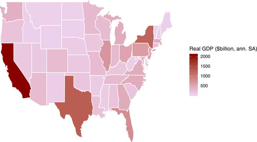
Figure 2. Real GDP Growth (% year-on-year) by State, average over 2005–2018.

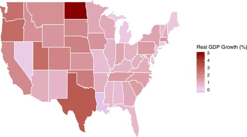
This disparity in the real GDP growth rates across states gives motivation for the inclusion of fixed effects in Eq. (2)(2) $$y_{i,t}={\alpha }_i+\sum _{s=1}^p{\gamma }_s^{\prime }{Y}_{i,t-s}+u_{i,t}$$(2) .

4.1.2. Monthly state-level employment data

We will use employment-related series as the main source of predictor variables in the MF-PVAR analysis. There are several reasons we use these in our analysis. First, employment-type series are amongst the most commonly-used predictors in previous empirical nowcasting studies. Secondly, this can serve as a proxy to labor income which is one of the key ingredients of the BEA’s methodology for constructing state-level GDP data. Finally, there are limited regional data on other typical nowcast predictors such as industrial production.

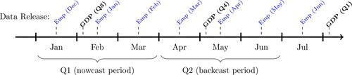
The Bureau of Labor Statistics (BLS) produces monthly state-level data for employees on nonfarm payrolls through the Current Employment Statistics (CES) programme, and state unemployment through the Local Area Unemployment Statistics (LAUS) programme.¹² The fact that these data are monthly makes them ideal candidates for use in nowcasting, particularly as the data are released in a much more timely fashion than real GDP, being available around a month and a half after the end of the reference month. This flow of data, depicted in Fig. 3, means that we have data on all three months of a given quarter well in advance of the same quarter’s GDP data release. This can allow us to build up an early picture of state-level GDP.

Figure 3. Graphical illustration of the data flow in predicting Q1.

4.2. Pseudo out-of-sample set-up

We will perform a panel pseudo out-of-sample evaluation to see how our proposed methods compare to competitors throughout history. As is customary in the nowcasting literature since studies such as Giannone et al. (2008), we will assess the performance of our models in making predictions at different points in the data flow depicted in Fig. 3. Specifically, we will make three different predictions per quarter of interest: a forecast, a nowcast and a backcast. These will be made roughly in the middle of the quarter, just after the release of GDP data, when the employment data for all three months of the previous quarter are available. As an example, looking at Fig. 3, the backcast of Q1 will be made in the middle of Q2 just after the release of the Q4 GDP data when all three months of the employment data for Q1 are available. Similarly, the nowcast of Q1 is made in the middle of Q1 and the forecast is made in the middle of Q4.

We first transform the data to stationarity using the year-on-year growth rates of the series which is the same growth rate as that presented by the BEA. This gives a final time series dimension of T = 49 quarterly observations for real GDP growth (denoted $gd{p}_{i,t}$) and $3T=147$ for the monthly employment and unemployment variables (denoted ${\text{emp}}_{i,t}$ and ${\text{unem}}_{i,t}$ respectively). The use of the year-on-year transformation is in line with other nowcasting studies which follow the year-on-year growth rate convention used by the relevant statistical authority, including Dahlhaus et al. (2017) and Bragoli and Fosten (2018). However, we will also compare our results to those using the quarter-on-quarter real GDP growth rate which is more common in studies which nowcast national aggregates.

To perform the out-of-sample evaluation we split the sample in the time series dimension into $T=R+P$ observations. We use the first R quarters of the data to estimate the models and make the backcasts, nowcasts and forecasts across the n states for quarter R + 1 and then proceed in a recursive fashion, adding one quarter of data at a time and re-estimating the parameters (including the bias correction) and the predictions throughout the remainder of the sample. As a central scenario, we start making out-of-sample nowcasts in 2012Q1 which splits the sample equally, giving a total of P = 25 quarters of evaluation over the n states and an initial estimation window of R = 24 quarters. To assess robustness to the choice of sample split, we will also report present results where nowcasting commences in 2010Q1 ($R=16,P=33$) and 2014Q1 ($R=32,P=17$). We will also check robustness to the use of the rolling estimation scheme, where the estimation window is held fixed at R quarters, unlike the recursive scheme where the window expands by one quarter at a time. Since we are estimating the models using small estimation windows in the time series dimension relative to the cross-section dimension, we are in a situation where bias correction is particularly relevant.

For the monthly endogenous explanatory variables in the MF-PVAR we will try both $x_{i,t}:={\text{emp}}_{i,t}$ and $x_{i,t}:={\text{unem}}_{i,t}.$¹³ For the lag specification, we will search over models up to $p^{\text{max}}=4$ lags to allow up to annual dynamics. For the BCLS MF-PVAR nowcasts we use four methods: lag selection using the panel FPE criterion above (denoted “MF-PVAR(FPE)” in the results), the Mallows model averaging method (“MF-PVAR(MMA)”), equal-weights forecast averaging (“MF-PVAR(EW)”) and a bias-corrected panel VAR(1) model (“MF-PVAR(1)”) which fixes the lag length at p = 1 in every period and does not select lags optimally. In order to compare BCLS with simple OLS (nonbias corrected) predictions, we will also present the MF-PVAR results where OLS is used for model estimation with a naïve BIC criterion (“MF-PVAR(BIC)”), details of which can be found in the Supplementary Material.

We will also report results for three benchmark methods. First, in order to assess the importance of the pooled panel approach, we will report results where individual time series OLS nowcasting regressions are run for each state (“MIDAS(1)”). This is like an unrestricted version of the MIDAS model of Clements and Galvão (2008, 2009) and corresponds to estimating Eq. (2)(2) $$y_{i,t}={\alpha }_i+\sum _{s=1}^p{\gamma }_s^{\prime }{Y}_{i,t-s}+u_{i,t}$$(2) state-by-state instead of pooling the data across states. Since the sample size for time series regression will be as low as R = 16, we restrict the number of parameters by fixing the lag length to be p = 1, which we denote the MIDAS(1) model. Finally, we will use two univariate benchmarks: a panel AR(1) model with homogeneous AR(1) coefficient estimated by OLS, and a time series AR(1) model which does not pool the information across states. The AR(1) model with no additional predictors is the most commonly-used benchmark in nowcasting studies, which is why we assess the performance of our methods relative to the panel and time series version of this benchmark.

In measuring the accuracy of the nowcasts across the various competing methods, we will use the MSFE criterion which averages the squared nowcast errors across the n states and the P evaluation periods.¹⁴ The unweighted MSFE is also used as the evaluative criterion for panel nowcasts in the papers of Babii et al. (2020) and Koop et al. (2020). If we generically define ${\widehat{u}}_{i,t}=y_{i,t}-{\widehat{y}}_{i,t}$ as the nowcast errors from any of the above methods, then we calculate MSFE as: (9) $$\text{MSFE}=\frac{1}{nP}\sum _{i=1}^n\sum _{t=R+1}^T{\widehat{u}}_{i,t}^2$$(9)

Finally, we will also explore the results by way of a subgroup analysis, where we restrict the sample of states to selected groups of size smaller than n. This is to check the impact of the homogeneous coefficients assumption on the results. The groupings will be discussed in more detail later.

4.3. Results: pseudo out-of-sample nowcast evaluation

4.3.1. Results across all states

We first present the main set of results where we compare the panel nowcasting methods estimated on information pooled across all states. The results of the pseudo out-of-sample evaluation of the forecasts, nowcasts and backcasts are displayed in Table 2. This shows the average MSFE across all states for each of the methods, first for the employment version of the model (top panel) and then for the unemployment version (bottom panel). There are several key findings to draw out of these results.

Table 2. MSFE Results: recursive estimation.

Predictor variable: ${\text{emp}}_{i,t}$
			$R=16,P=33$			$R=24,P=25$			$R=32,P=17$
			Forecast	Nowcast	Backcast	Forecast	Nowcast	Backcast	Forecast	Nowcast	Backcast
Panel	BCLS	MF-PVAR(FPE)	6.572	4.007	2.162	5.009	3.300	1.926	3.603	2.263	1.154
		MF-PVAR(MMA)	6.571	4.007	2.162	5.009	3.300	1.926	3.603	2.263	1.154
		MF-PVAR(EW)	5.031	3.356	2.068	4.490	3.086	1.918	3.234	2.129	1.134
		MF-PVAR(1)	5.214	3.557	2.247	4.557	3.282	2.044	3.080	2.194	1.213
Panel	OLS	MF-PVAR(BIC)	6.905	4.336	2.256	5.269	3.468	1.979	3.981	2.416	1.191
		Panel AR(1)	6.097	4.228	2.409	5.254	3.754	2.243	4.029	2.859	1.447
TS	OLS	MIDAS(1)	7.004	4.780	2.911	5.481	3.975	2.455	3.972	2.836	1.609
		AR(1)	7.365	4.551	2.433	5.984	4.065	2.302	3.907	2.791	1.438
Predictor variable: ${\text{unem}}_{i,t}$
			$R=16,P=33$			$R=24,P=25$			$R=32,P=17$
			Forecast	Nowcast	Backcast	Forecast	Nowcast	Backcast	Forecast	Nowcast	Backcast
Panel	BCLS	MF-PVAR(FPE)	6.609	4.439	2.400	5.929	4.047	2.217	4.850	3.152	1.530
		MF-PVAR(MMA)	6.602	4.439	2.401	5.929	4.047	2.217	4.850	3.152	1.530
		MF-PVAR(EW)	5.550	3.944	2.328	5.123	3.655	2.181	4.104	2.826	1.444
		MF-PVAR(1)	5.646	4.092	2.416	5.116	3.717	2.238	3.807	2.737	1.440
Panel	OLS	MF-PVAR(BIC)	7.154	4.844	2.517	6.295	4.298	2.292	5.222	3.344	1.592
		Panel AR(1)	6.097	4.228	2.409	5.254	3.754	2.243	4.029	2.859	1.447
TS	OLS	MIDAS(1)	8.814	5.844	3.144	7.078	4.860	2.722	3.970	2.835	1.640
		AR(1)	7.365	4.551	2.433	5.984	4.065	2.302	3.907	2.791	1.438

We first note that the idea of incorporating timely information is important for nowcasting. We can see from the top panel of Table 2 that the MF-PVAR models with employment have substantially lower MSFE on average than the panel or time series AR(1) methods. For example, in the case where $R=24,P=25,$ the BCLS MF-PVAR(1) method gives uniformly lower MSFE than the panel AR(1) method by a factor of 9% for the backcast and around 13% for both the nowcast and forecast. This result is robust to the choice of R and P with even larger relative MSFE gains in the case of $R=32,P=17.$ On the other hand, looking at the lower panel of Table 2 we see that the unemployment version of the model fares much worse than the employment version of the model, typically with 10%–30% higher MSFE depending on the method. This indicates that employment growth provides a better timely signal than the unemployment rate, and we will focus on these results in what follows.

In relation to the bias-corrected methods, there are two main points to draw out of Table 2. We first note that the backcasts are improved by the use of model selection or combination yields, relative to fixing the number of lags at p = 1 as is done in the BCLS MF-PVAR(1) method. We especially note that the equal weights forecast combination method MF-PVAR(EW) delivers the lowest MSFE across forecast, nowcast and backcast with the exception of the $R=32,P=17$ case. In some cases the gain is well above 20% relative to the panel AR(1) model. This indicates that the use of forecast combination in conjunction with BCLS can be a very useful method in making state-level nowcasts of real GDP growth. Secondly, we find that the bias correction is, indeed, beneficial since the BCLS method using FPE results in lower MSFE than the equivalent use of OLS with the standard BIC selection criterion. The improvement is in the range 5–10% across all of the results in the top panel of Table 2. We expect gains from bias correction to be even larger in other applications where the overall time series dimension T is yet smaller.

Finally, a very important result is that there appear to be substantial gains from pooling information across states in our panel nowcasting approach. The MIDAS(1) model, which uses employment information in state-by-state time series regressions, performs poorly relative to the panel methods and even relative to the time series AR(1) method in some cases. The fact that the MIDAS(1) and time series AR(1) are the worst performing methods across most of the results in Table 2 illustrates the benefits from pooling information across states rather than obtaining predictions from time series models with few observations and many parameters.

In addition to displaying the robustness of the results to the choice of R and P, in Table 3 we also report results where we change to the rolling parameter estimation scheme. This is where the estimation window is held fixed at R time series observations rather than expanding the window one-by-one as in the recursive scheme. Focusing again on the employment version of the model, in the top panel of Table 3 we see that the MSFE is larger than that of recursive estimation in all cases. For instance, taking the BCLS MF-PVAR(1) method for $R=24,P=25,$ the rolling scheme gives 8% higher MSFE for the backcast, 15% higher for the nowcast and 20% higher for the forecast. The gap is even larger when R = 16 which highlights the need to use the maximum number of observations possible in estimating the models. Also, we see huge inflation of MSFE for the time series MIDAS(1) and AR(1) models as these are only estimated on a small window of observations which does not grow as in the recursive scheme. We therefore would not recommend the use of rolling estimation in panels with similar dimensions to these. That being said, the results are qualitatively similar in the sense that the BCLS MF-PVAR methods typically deliver the lowest MSFE in the employment model, especially in the equal weights forecast averaging method.

Table 3. MSFE results: rolling estimation.

Predictor variable: ${\text{emp}}_{i,t}$
			$R=16,P=33$			$R=24,P=25$			$R=32,P=17$
			Forecast	Nowcast	Backcast	Forecast	Nowcast	Backcast	Forecast	Nowcast	Backcast
Panel	BCLS	MF-PVAR(FPE)	9.601	4.926	2.362	5.557	3.530	2.023	3.717	2.361	1.241
		MF-PVAR(MMA)	9.240	4.821	2.336	5.534	3.509	2.017	3.716	2.359	1.239
		MF-PVAR(EW)	6.000	3.604	2.104	5.027	3.288	1.988	3.388	2.237	1.187
		MF-PVAR(1)	6.374	4.115	2.403	5.488	3.779	2.202	3.286	2.323	1.261
Panel	OLS	MF-PVAR(BIC)	9.295	5.258	2.520	5.509	3.628	2.086	4.135	2.548	1.301
		Panel AR(1)	6.275	4.396	2.485	5.383	3.885	2.321	4.118	2.901	1.447
TS	OLS	MIDAS(1)	10.023	7.054	4.448	6.024	4.477	2.996	4.122	3.015	1.807
		AR(1)	7.824	4.818	2.560	6.215	4.190	2.367	4.050	2.875	1.479
Predictor Variable: ${\text{unem}}_{i,t}$
			$R=16,P=33$			$R=24,P=25$			$R=32,P=17$
			Forecast	Nowcast	Backcast	Forecast	Nowcast	Backcast	Forecast	Nowcast	Backcast
Panel	BCLS	MF-PVAR(FPE)	7.962	4.763	2.510	6.199	4.144	2.270	4.899	3.167	1.561
		MF-PVAR(MMA)	7.789	4.710	2.499	6.176	4.131	2.269	4.898	3.166	1.560
		MF-PVAR(EW)	5.937	3.994	2.336	5.327	3.774	2.244	4.231	2.880	1.462
		MF-PVAR(1)	6.268	4.467	2.539	5.333	3.891	2.320	4.020	2.867	1.475
Panel	OLS	MF-PVAR(BIC)	8.760	5.499	2.823	6.776	4.533	2.415	5.357	3.426	1.655
		Panel AR(1)	6.275	4.396	2.485	5.383	3.885	2.321	4.118	2.901	1.447
TS	OLS	MIDAS(1)	11.982	8.366	5.134	8.706	6.016	3.278	4.425	3.212	1.944
		AR(1)	7.824	4.818	2.560	6.215	4.190	2.367	4.050	2.875	1.479

We also ran results for the quarter-on-quarter growth rate which, although not reported by the BEA in the context of state-level GDP growth, is often used by researchers interested in national aggregate real GDP growth. The results can be found in Table S11 in the Supplementary Material. These show qualitatively similar findings to the year-on-year results above, where the model with employment data seems to perform better than unemployment data. The gains from nowcasting, relative to autoregressive benchmarks, appear to be slightly smaller than in the year-on-year case, but can still be over 20%, for example the backcast results for the $R=35,P=17$ case.

4.3.2. State-level results

Rather than focusing on the nowcast model performance on average across states, it is interesting to zoom in and see how the models perform within specific states. To achieve this we can also present the MSFE results from Table 2 for individual states, acknowledging that this is based on a relatively small quarterly time series sample. For this reason, we now turn attention to the results with the largest evaluation window $P=33.$

Returning to the four states with highest real GDP from Table 1 above, Table 4 presents the benchmark results as in Table 2 but for these four states. We can see from these results that the BCLS MF-PVAR methods also perform the best when looking at these individual states, delivering the lowest MSFE in 11 out of the 12 cases. Again, it appears that the use of lag selection can, in fact, give larger MSFE in the forecast and nowcast periods and the BCLS MF-PVAR(1) method gives the lowest MSFE in many cases.

Table 4. MSFE results: largest four states.

			California			Florida
			Forecast	Nowcast	Backcast	Forecast	Nowcast	Backcast
Panel	BCLS	MF-PVAR(FPE)	2.853	1.931	0.937	5.201	2.138	0.996
		MF-PVAR(MMA)	2.856	1.931	0.937	5.202	2.138	0.996
		MF-PVAR(EW)	1.997	1.504	0.903	3.484	1.716	1.071
		MF-PVAR(1)	2.099	1.335	0.877	2.587	1.479	1.163
Panel	OLS	MF-PVAR(BIC)	3.332	2.128	0.929	5.466	2.405	1.001
		Panel AR(1)	4.013	2.604	1.317	4.796	2.893	1.530
TS	OLS	MIDAS(1)	1.898	1.589	1.190	5.985	3.561	1.775
		AR(1)	3.761	2.486	1.295	3.815	2.273	1.349
			New York			Texas
			Forecast	Nowcast	Backcast	Forecast	Nowcast	Backcast
Panel	BCLS	MF-PVAR(FPE)	3.545	2.084	1.543	4.425	2.438	1.031
		MF-PVAR(MMA)	3.524	2.084	1.543	4.426	2.438	1.031
		MF-PVAR(EW)	2.149	1.687	1.408	3.672	2.372	1.080
		MF-PVAR(1)	3.147	2.416	1.692	3.566	2.336	1.252
Panel	OLS	MF-PVAR(BIC)	2.947	2.201	1.634	5.067	2.631	1.060
		Panel AR(1)	3.344	2.988	1.929	4.693	3.080	1.359
TS	OLS	MIDAS(1)	5.944	4.070	2.261	4.097	2.684	1.541
		AR(1)	3.281	2.954	1.869	5.725	3.279	1.352

These results are for the model with employment as the single predictor, and for $R=16,P=33$ with recursive estimation.

We also see that there is considerable variation in the performance of the time series MIDAS(1) models. In some cases the MIDAS(1) method appears better than the average we see in Table 2, and in some cases worse. For instance, in Texas the MIDAS(1) method gets close to the MF-PVAR methods in terms of MSFE. On the other hand, for New York we see that the results are much worse for the MIDAS(1), with almost 80% higher MSFE than the panel AR(1) in the forecast column. The variation in these results seems to gives some motivation toward exploring the assumption of homogeneity of the panel model coefficients which we impose in Eq. (2)(2) $$y_{i,t}={\alpha }_i+\sum _{s=1}^p{\gamma }_s^{\prime }{Y}_{i,t-s}+u_{i,t}$$(2) . We will explore this in more detail in a later section.

Finally, in addition to exploring the state-level results in these four important cases, we can also shed further light by looking at the distribution of MSFE across all states. In the Supplementary Material, we display histograms (Figures S5, S7 and S9) representing the distribution of the MSFE across states for forecast, nowcast and backcast, corresponding to the results in Table 2. We also present the same histograms but for the MSFE relative to the panel AR(1) model (Figures S6, S8 and S10) which are less prone to the outliers seen in the raw MSFE histograms. These results confirm that the equal-weights forecast averaging method MF-PVAR(EW) seems to perform well across forecast, nowcast and backcast, with the bulk of the MSFE distribution being to the left of all of the other methods. The results also serve to highlight that there can be extreme outliers when using the nonpooled time series AR(1) method instead of using pooled panel methods. This is evident especially in the nowcast and forecast results where the highest MSFE for the time series AR(1) method is more than double that of the equal-weights method.

4.3.3. Exogenous national-level predictors

It is possible that the predictions of real GDP growth across states can be improved by incorporating variables related to national business cycle movements. Similar arguments are used in a different context by Koop et al. (2020) who nowcast regional GVA in the U.K. using national GVA. On the other hand, the opposite approach is taken in the U.S. by Gonzalez-Astudillo (2019) who uses state-level data to estimate national business cycles.

We therefore add in national real GDP growth as an exogenous variable into the mixed frequency VAR methods. This also gives us the opportunity to explore the modified bias correction which holds in the presence of exogenous predictors, as outlined above. The results are displayed in Table 5 which contains the MSFE results for the employment model and for the $R=16,P=33$ case. These results can be compared to the upper left panel of Table 2 which show the equivalent set of results without the exogenous national GDP predictor. This seems to suggest that we do not gain a lot by adding in the exogenous national variable. Focusing on the equal weights forecast averaging method, which delivers the best results generally, we see an improvement in MSFE over Table 2 of around 4% for the backcast, 1% for the nowcast and a worsening of around 20% for the forecast. Overall, while there may be some small gains to be had from adding in national predictors to regional nowcasting models in the U.S., further work should be done to explore the circumstances of these improvements.

Table 5. MSFE Results: - exogenous national GDP.

			Forecast	Nowcast	Backcast
Panel	BCLS	MF-PVAR(FPE)	9.805	4.184	2.102
		MF-PVAR(MMA)	9.664	4.154	2.096
		MF-PVAR(EW)	6.230	3.306	1.983
		MF-PVAR(1)	5.436	3.549	2.214
Panel	OLS	MF-PVAR(BIC)	6.836	4.094	2.182
		Panel AR(1)	6.097	4.228	2.409
TS	OLS	MIDAS(1)	10.787	6.153	3.413
		AR(1)	7.365	4.551	2.433

These numbers display the MSFE for the model with employment as the single predictor, and for $R=16,P=33$ with recursive estimation. The Panel and Time Series AR(1) methods give the same MSFE as in Table 2 as they do not use any additional predictors.

4.3.4. Allowing heterogeneity: sub-group pooling versus all-states pooling

The results of the MF-PVAR nowcasting models up until now have used information pooled across all n = 50 states under the assumption that each state has homogeneous slope coefficients in Eqs. (1)(1) $$Y_{i,t}={\mu }_i+\sum _{s=1}^p{\Lambda }_s^{\prime }{Y}_{i,t-s}+U_{i,t},$$(1) and (2)(2) $$y_{i,t}={\alpha }_i+\sum _{s=1}^p{\gamma }_s^{\prime }{Y}_{i,t-s}+u_{i,t}$$(2) . We also found that it was not advisable to allow heterogeneity by estimating individual time series equations when the sample size is prohibitively low. In this section we explore whether there is any merit to pooling across specific subgroups of states, as an intermediate step between all-state pooling and time series estimation.

In dividing the U.S. states into smaller subgroups there are many possibilities. The first, and perhaps most obvious, way to categorize is based on geographical regions. We therefore break down the states into the U.S. Census Bureau’s four census regions: Northeast ($n_1=9$), Midwest ($n_2=12$), South ($n_3=16$) and West ($n_4=13$).¹⁵ Other categorizations we consider are those discussed in Greenaway-McGrevy and Hood (2019) which are based on states with similar production characteristics. As such we will look at energy-producing states ($n_1=7$) as well as the so-called “Rust Belt” states ($n_2=7$) which experienced common industrial decline since the 1980s. For completeness we will also report an “Other” subgroup ($n_3=36$) which excludes both energy and Rust Belt states. These groupings are displayed in Table S10 in the Supplementary Material. To avoid only using pre-determined groups, we also check our results using a data-driven method suggested by Su et al. (2016) which identifies latent subgroup structures in panel data using a classifier-Lasso (C-Lasso).

Table 6 displays the MSFE results from sub-group pooling versus all-states pooling for the backcast and for the model with employment as the single predictor with recursive estimation and sample split $R=16,P=33.$ The nowcast and forecast results can be found in Tables S12 and S13 in the Supplementary Material. To produce these results, we first estimate the panel models (MF-PVAR and panel AR(1)) only using the sub-group data and report the average MSFE for that sub-group. We then take the results from the all-states estimation (as used in Table 2) and report the average MSFE measure for the same sub-group. This helps us to gauge whether results improve if we strip out extra states, or whether pooling additional information from other states can improve estimation and therefore the predictions in particular sub-groups.

Table 6. Backcast MSFE results: sub-group pooling vs. all-states pooling.

			Northeast		Midwest		South		West
			Sub-group	All-states	Sub-group	All-states	Sub-group	All-states	Sub-group	All-states
Panel	BCLS	MF-PVAR(FPE)	3.065	1.688	3.047	2.730	1.827	1.703	2.963	2.531
		MF-PVAR(MMA)	2.091	1.688	2.941	2.730	1.816	1.703	2.846	2.531
		MF-PVAR(EW)	1.641	1.719	2.788	2.721	1.819	1.674	2.406	2.191
		MF-PVAR(1)	1.891	1.838	3.145	3.060	2.013	1.962	2.183	2.131
Panel	OLS	MF-PVAR(BIC)	2.157	1.692	3.047	2.810	2.080	1.750	2.939	2.757
		Panel AR(1)	1.889	1.971	3.465	3.448	1.957	1.936	2.312	2.335
TS	OLS	MIDAS(1)	2.292	–	3.577	–	2.658	–	3.036	–
		AR(1)	1.835	–	3.499	–	2.060	–	2.322	–
			Rust Belt		Energy		Other
			Sub-group	All-states	Sub-group	All-states	Sub-group	All-states
Panel	BCLS	MF-PVAR(FPE)	2.010	1.478	4.879	4.328	1.942	1.874
		MF-PVAR(MMA)	1.726	1.478	4.338	4.328	1.923	1.874
		MF-PVAR(EW)	1.514	1.419	3.831	3.933	1.818	1.831
		MF-PVAR(1)	1.893	1.672	4.258	4.335	1.958	1.953
Panel	OLS	MF-PVAR(BIC)	1.459	1.520	4.221	4.806	1.960	1.903
		Panel AR(1)	1.673	1.651	5.208	5.270	1.994	2.000
TS	OLS	MIDAS(1)	2.280	–	5.479	–	2.534	–
		AR(1)	1.689	–	5.507	–	1.980	–

These numbers display the MSFE by subgroup for the model with employment as the single predictor, and for $R=16,P=33$ with recursive estimation. The “Sub-group” column shows the MSFE results for that sub-group of states, and where the panel models are estimated only using data from that that sub-group. The “All-states” column gives the MSFE results for the same sub-group of states, but where the panel models are estimated using data from all states. Since the time series (TS) models are estimated state-by-state the results are the same across these two columns, so one entry is replaced with “–” to avoid confusion.

The striking result from Table 6 is that there appears to be no evidence in favor of using sub-group pooling as a way to allow for heterogeneity in the coefficients. In fact, the opposite result holds that the MSFE actually tends to be lower when all-states pooling is used to estimate the parameters of the model. These gains from all-states pooling are typically in the region of 5% to 10% but can be as large as 40% in some cases. The nowcast and forecast results in the Supplementary Material show even worse results for the sub-group estimation, perhaps because they iterate forward the estimates from very small samples. This result is in favor of our baseline approach for modeling the panel by pooling across all states with homogeneous coefficients.

Overall, these results indicate that in relatively small panels like this, the gains from pooling information across all states appear to outweigh any improvement from permitting heterogeneity across subgroups. This provides further evidence in favor of pooling in the “to pool or not to pool” debate posed by Wang et al. (2019) and others. We also note that we find similar results when using a data-driven selection of the subgroups using the C-Lasso approach of Su et al. (2016) instead of these pre-determined subgroups.¹⁶

In looking across the geographical regions, the worsening from subgroup pooling is lowest in the South, which is the region with the largest number of states. This also gives evidence that pooling across a large estimation sample size is more important than allowing heterogeneity in this example. In the lower panel of Table 6 a similar story emerges in that the largest “Other” category gives similar results between sub-group and all-state pooling. As a final extension to explore subgroup pooling, we added in the inflation in the West Texas Intermediate (WTI) crude oil price as an exogenous variable into the MF-PVAR for energy-producing states to see if this yielded any MSFE improvements.¹⁷ While there were some minimal improvements in the order of 1–2% gain in MSFE for some of the methods, we did not find any substantial and consistent improvements in adding this as an exogenous predictor.

5. Conclusion

In this article, we look to shift the attention of the existing nowcasting literature away from time series methods to the panel data context. This allows us to perform near-term prediction of regional or sectoral data which typically suffer from even worse issues with data timeliness than national aggregate data such as real GDP. In our empirical application we find clear gains from pooling information using panel methods when the purpose is nowcasting U.S. state-level GDP growth.

We propose a mixed-frequency panel VAR approach to nowcasting and demonstrate how the model can be estimated using a BCLS approach. We also suggest several model selection and combination methods, building on recent panel forecasting research by Greenaway-McGrevy (2019, 2020, 2022). Since the model selection methods have not been developed in a mixed-frequency framework, we are careful to demonstrate, though Monte Carlo simulation, the effectiveness of these model selection methods relative to naïve benchmarks. Our application to U.S. state-level GDP nowcasting yields further insights than previous national studies which cannot give state-level information, and highlights the usefulness of pooling information across states. We envisage many further possible applications of our methods, such as the prediction of sectoral GDP or nowcasting multiple different proxies for inflation.

Further work may look to enhance this panel nowcast model specification by allowing factors to be estimated from a large set of external (time series) variables, or to estimate a common factor from the panel of endogenous variables itself. This would extend existing factor-based time series nowcasting methods (see Antolin Diaz et al., 2017; Banbura et al., 2013; Fosten and Gutknecht, 2020; Giannone et al., 2008) to the panel data context.

Acknowledgments

The authors are grateful for very useful comments from the editor, associate editor and three anonymous referees, as well as discussions with Michael Clements, Ana Galvão, Ivan Petrella, Gary Koop, Kalvinder Shields, Domenico Giannone, Dean Croushore, Shaun Vahey, Eleanora Granziera, Kevin Lee and participants at the workshops: “Advances in Economic Modelling and Forecasting” at Warwick Business School (July 2019) and “Real-Time Data Analysis, Methods and Applications” at the National Bank of Belgium (October 2019).

Correction Statement

This article has been republished with minor changes. These changes do not impact the academic content of the article.

Notes

1 This is as opposed to model selection for the purpose of inference after incidental parameters have been integrated out (Greenaway-McGrevy, 2019).

2 This is something we explore later in the Monte Carlo and empirical application.

3 Clearly the number of parameters in Λ_s grows with the frequency of the $x_{i,t}$ variables. This could result in over-parameterisation if, for example, daily data were to be stacked alongside the quarterly variable. On the other hand, papers like Baumeister et al. (2015) have suggested to incorporate daily data into this stacked VAR model simply by using the weekly aggregation of the daily data.

4 For instance, if only the second month of data for quarter t were available ($x_{i,t-1/3}$) but not the third month ($x_{i,t}$) then one could instead re-specify the vector $Y_{i,t}:={(y_{i,t},x_{i,t+2/3},x_{i,t+1/3},x_{i,t})}^{\prime }.$ Equation (2) would then relate $y_{i,t}$ to $x_{i,t-1/3},$ $x_{i,t-2/3}$ and $x_{i,t-1}$ as well as $y_{i,t-1}.$ The fact that this stacked MIDAS-type approach requires the model to be re-specified at different nowcast points can be considered a drawback relative to the state space approaches mentioned above. On the other hand, the stacked method does not require the estimation of the latent high-frequency equivalent of the low-frequency variable.

5 OLS estimates of the fixed effects are also biased, although most of the extant literature focuses on the bias in the estimates of common parameters.

6 This method corresponds to an iterative forecast. An alternative is the direct forecast, which is generated from a model tailored to the forecast horizon. This can be obtained by replacing $Y_{i,t}$ in Eq. (1) with $Y_{i,t+h-1}.$ Greenaway-McGrevy (2020) provides formulae for the associated bias correction and model selection criteria for choosing p. Under misspecification the direct forecast exhibits a lower asymptotic MSFE than the iterative forecast. However, in the finite sample, it is unclear whether the direct forecast will have a smaller MSFE because the variance of the iterative forecast is less than that of the direct forecast for a given lag length. See Greenaway-McGrevy (2013) for further details. Thus, the iterative (direct) forecast will be more accurate if the degree of misspecification is sufficiently small (large). Introducing data-determined lag selection or model averaging for each method compounds the difficultly of ranking the two methods.

7 Greenaway-McGrevy (2019) shows that the maximum permissible rate of expansion in the lag order is just slower than $\max \left(\sqrt{n},\sqrt{T}\right).$ This lag order selection rule ensures that $p_{\max }$ grows at a rate just above this maximum permissible rate.

8 This is the MSFE of an infinitely large model with known (not estimated) parameters.

9 See https://www.philadelphiafed.org/research-and-data/regional-economy/indexes/coincident. Last accessed 07 August 2020.

10 See https://www.bea.gov/data/gdp/gdp-state. Last accessed 25 October 2018.

11 See https://apps.bea.gov/regional/histdata/. Last accessed 04 May 2021.

12 See https://www.bls.gov/sae/ and https://www.bls.gov/lau/. Last accessed 25 October 2018.

13 Earlier versions of the paper also checked the results when both predictors were used and $x_{i,t}:={[{\text{emp}}_{i,t},{\text{unem}}_{i,t}]}^{\prime }.$ The results did not improve over the main results and these models involved the estimation of more parameters.

14 We do not assess the statistical significance of the MSFE differences between models as in Diebold and Mariano (1995) and West (1996). Although there have been recent papers looking at panel versions of the Diebold-Mariano (DM) test for pairwise comparisons (Timmermann and Zhu, 2019; Akgun et al., 2020), they are not applicable in our context which looks at multiple different forecast methods with no single ‘benchmark’ model (like Hansen et al., 2011, provide in the time series context). Additionally, the contribution of parameter estimation to DM tests has not yet been explored in a panel context, which is particularly relevant in our case with small panel dimensions and the introduction of an estimated bias correction.

15 See https://www2.census.gov/geo/pdfs/maps-data/maps/reference/us_regdiv.pdf. Last accessed 17 July 2019.

16 Specifically, we find that the C-Lasso approach predominantly picks out a very small subgroup of three energy-producing states when it is used to identify two latent sub-groups: Alaska, North Dakota and Wyoming. When we run the results for this small subgroup the results are poor relative to the all-state pooled results, presumably due to the very small sample size for estimation. The results are therefore not presented here, but are available on request.

17 Data accessed from FRED Economic Data: https://fred.stlouisfed.org/series/DCOILWTICO. Last accessed 17 September 2019.

References

- Aastveit, K. A., Gerdrup, K. R., Jore, A. S., Thorsrud, L. A. (2014). Nowcasting GDP in real time: a density combination approach. Journal of Business & Economic Statistics 32(1):48–68. doi:https://doi.org/10.1080/07350015.2013.844155
- Aastveit, K. A., Ravazzolo, F., Van Dijk, H. K. (2018). Combined density nowcasting in an uncertain economic environment. Journal of Business & Economic Statistics 36(1):131–145. doi:https://doi.org/10.1080/07350015.2015.1137760
- Akgun, O., Pirotte, A., Urga, G., Yang, Z. (2020). Equal predictive ability tests for panel data with an application to OECD and IMF forecasts. arXiv Preprint arXiv:2003.02803.
- Antolin Diaz, J., Drechsel, T., Petrella, I. (2017). Tracking the slowdown in long-run GDP growth. The Review of Economics and Statistics 99(2):343–356. doi:https://doi.org/10.1162/REST_a_00646
- Babii, A., Ball, R. T., Ghysels, E., Striaukas, J. (2020). Machine learning panel data regressions with an application to nowcasting price earnings ratios. arXiv:2008.03600v1
- Baffigi, A., Golinelli, R., Parigi, G. (2004). Bridge models to forecast the euro area GDP. International Journal of Forecasting 20(3):447–460. doi:https://doi.org/10.1016/S0169-2070(03)00067-0
- Baltagi, B. H. (2008). Forecasting with panel data. Journal of Forecasting27(2):153–173. doi:https://doi.org/10.1002/for.1047
- Baltagi, B. H., Griffin, J. M. (1997). Pooled estimators vs. their heterogeneous counterparts in the context of dynamic demand for gasoline. Journal of Econometrics 77(2):303–327. doi:https://doi.org/10.1016/S0304-4076(96)01802-7
- Banbura, M., Giannone, D., Modugno, M., Reichlin, L. (2013). Now-casting and the real-time data flow. In: Elliott, G. Timmermann, A., eds., Handbook of Economic Forecasting, vol. 2A. Amsterdam: North-Holland, pp. 195–236.
- Baumeister, C., Guérin, P., Kilian, L. (2015). Do high-frequency financial data help forecast oil prices? The MIDAS touch at work. International Journal of Forecasting 31(2):238–252. doi:https://doi.org/10.1016/j.ijforecast.2014.06.005
- Bhansali, R. J. (1997). Direct autoregressive predictors for multistep prediction: order selection and performance relative to the plug in predictors. Statistica Sinica 7(2):425–449.
- Binder, M., Krause, M. (2014). Mixed frequency panel vector autoregressions and the inequality vs. Growth nexus. Mimeo.
- Bok, B., Caratelli, D., Giannone, D., Sbordone, A. M., Tambalotti, A. (2018). Macroeconomic nowcasting and forecasting with big data. Annual Review of Economics10(1):615–643. doi:https://doi.org/10.1146/annurev-economics-080217-053214
- Bragoli, D., Fosten, J. (2018). Nowcasting Indian GDP. Oxford Bulletin of Economics and Statistics80(2):259–282. doi:https://doi.org/10.1111/obes.12219
- Brave, S. A., Butters, R. A., Justiniano, A. (2019). Forecasting economic activity with mixed frequency BVARs. International Journal of Forecasting 35(4):1692–1707. doi:https://doi.org/10.1016/j.ijforecast.2019.02.010
- Chudik, A., Pesaran, M. H., Tosetti, E. (2011). Weak and strong cross-section dependence and estimation of large panels. The Econometrics Journal14(1):C45–C90. doi:https://doi.org/10.1111/j.1368-423X.2010.00330.x
- Clements, M. P., Galvão, A. B. (2008). Macroeconomic forecasting with Mixed-Frequency data. Journal of Business & Economic Statistics 26(4):546–554. doi:https://doi.org/10.1198/073500108000000015
- Clements, M. P., Galvão, A. B. (2009). Forecasting US output growth using leading indicators: an appraisal using MIDAS models. Journal of Applied Econometrics24(7):1187–1206. doi:https://doi.org/10.1002/jae.1075
- Dahlhaus, T., Guénette, J.-D., Vasishtha, G. (2017). Nowcasting BRIC + M in real time. International Journal of Forecasting 33(4):915–935. doi:https://doi.org/10.1016/j.ijforecast.2017.05.002
- Diebold, F. X., Mariano, R. S. (1995). Comparing predictive accuracy. Journal of Business & Economic Statistics 13(3):253–263. doi:https://doi.org/10.2307/1392185
- Foroni, C., Guérin, P., Marcellino, M. (2018). Using low frequency information for predicting high frequency variables. International Journal of Forecasting 34(4):774–787. doi:https://doi.org/10.1016/j.ijforecast.2018.06.004
- Fosten, J., Gutknecht, D. (2020). Testing nowcast monotonicity with estimated factors. Journal of Business & Economic Statistics 38(1):107–123. doi:https://doi.org/10.1080/07350015.2018.1458623
- Ghysels, E. (2016). Macroeconomics and the reality of mixed frequency data. Journal of Econometrics 193(2):294–314. doi:https://doi.org/10.1016/j.jeconom.2016.04.008
- Ghysels, E., Sinko, A., Valkanov, R. (2007). MIDAS regressions: Further results and new directions. Econometric Reviews 26(1):53–90. doi:https://doi.org/10.1080/07474930600972467
- Giannone, D., Monti, F., Reichlin, L. (2016). Exploiting the monthly data flow in structural forecasting. Journal of Monetary Economics 84:201–215. doi:https://doi.org/10.1016/j.jmoneco.2016.10.011
- Giannone, D., Reichlin, L., Small, D. (2008). Nowcasting: the real-time informational content of macroeconomic data. Journal of Monetary Economics 55 (4):665–676. doi:https://doi.org/10.1016/j.jmoneco.2008.05.010
- Gonzalez-Astudillo, M. (2019). Estimating the US output gap with state-level data. Journal of Applied Econometrics 34(5):795–810.
- Greenaway-McGrevy, R. (2013). Multistep prediction of panel vector autoregressive processes. Econometric Theory29(4):699–734. doi:https://doi.org/10.1017/S0266466612000679
- Greenaway-McGrevy, R. (2019). Asymptotically efficient model selection for panel data forecasting. Econometric Theory 35(4):842–899. doi:https://doi.org/10.1017/S0266466618000294
- Greenaway-McGrevy, R. (2020). Multistep forecast selection for panel data. Econometric Reviews 39(4):373–406. doi:https://doi.org/10.1080/07474938.2019.1651490
- Greenaway-McGrevy, R. (2022). Forecast combination for VARs in large N and T panels. International Journal of Forecasting 38(1):142–164. doi:https://doi.org/10.1016/j.ijforecast.2021.04.006
- Greenaway-McGrevy, R., Hood, K. (2019). Aggregate effects and measuring regional dynamics. Papers in Regional Science 98(5):1955–1991. doi:https://doi.org/10.1111/pirs.12441
- Hahn, J., Kuersteiner, G. (2002). Asymptotically unbiased inference for a dynamic panel model with fixed effects when both n and T are large. Econometrica 70(4):1639–1657. doi:https://doi.org/10.1111/1468-0262.00344
- Hansen, P. R., Lunde, A., Nason, J. M. (2011). The model confidence set. Econometrica 79(2):453–497.
- Khalaf, L., Kichian, M., Saunders, C., Voia, M. (2021). Dynamic panels with MIDAS covariates: nonlinearity, estimation and fit. Journal of Econometrics 220(2):589–605. doi:https://doi.org/10.1016/j.jeconom.2020.04.015
- Koop, G., McIntyre, S., Mitchell, J. (2020). UK regional nowcasting using a mixed frequency vector auto-regressive model with entropic tilting. Journal of the Royal Statistical Society: Series A (Statistics in Society)183(1):91–119. doi:https://doi.org/10.1111/rssa.12491
- Kuzin, V., Marcellino, M., Schumacher, C. (2011). MIDAS vs. mixed-frequency VAR: nowcasting GDP in the euro area. International Journal of Forecasting 27(2):529–542. doi:https://doi.org/10.1016/j.ijforecast.2010.02.006
- Lee, Y. (2012). Bias in dynamic panel models under time series misspecification. Journal of Econometrics 169(1):54–60. doi:https://doi.org/10.1016/j.jeconom.2012.01.009
- Lee, Y., Phillips, P. C. B. (2015). Model selection in the presence of incidental parameters. Journal of Econometrics 188(2):474–489. doi:https://doi.org/10.1016/j.jeconom.2015.03.012
- Liu, L., Moon, H. R., Schorfheide, F. (2020). Forecasting with dynamic panel data models. Econometrica 88(1):171–201. doi:https://doi.org/10.3982/ECTA14952
- Mariano, R. S., Murasawa, Y. (2010). A coincident index, common factors, and monthly real GDP. Oxford Bulletin of Economics and Statistics 72(1):27–46. doi:https://doi.org/10.1111/j.1468-0084.2009.00567.x
- McCracken, M. W., Owyang, M., Sekhposyan, T. (2021). Real-time forecasting with a large, mixed frequency, Bayesian VAR. International Journal of Central Banking (71):327–367.
- Mouchart, M., Rombouts, J. V. K. (2005). Clustered panel data models: an efficient approach for nowcasting from poor data. International Journal of Forecasting 21(3):577–594. doi:https://doi.org/10.1016/j.ijforecast.2004.12.007
- Nickell, S. (1981). Biases in dynamic models with fixed effects. Econometrica 49(6):1417–1426. doi:https://doi.org/10.2307/1911408
- Pesaran, M. H. (2006). Estimation and inference in large heterogeneous panels with a multifactor error structure. Econometrica 74(4):967–1012. doi:https://doi.org/10.1111/j.1468-0262.2006.00692.x
- Pesaran, M. H., Shin, Y., Smith, R. P. (1999). Pooled mean group estimation of dynamic heterogeneous panels. Journal of the American Statistical Association 94(446):621–634. doi:https://doi.org/10.1080/01621459.1999.10474156
- Pesaran, M. H., Smith, R. (1995). Estimating long-run relationships from dynamic heterogeneous panels. Journal of Econometrics 68(1):79–113. doi:https://doi.org/10.1016/0304-4076(94)01644-F
- Phillips, P. C. B., Sul, D. (2007). Bias in dynamic panel estimation with fixed effects, incidental trends and cross section dependence. Journal of Econometrics 137(1):162–188. doi:https://doi.org/10.1016/j.jeconom.2006.03.009
- Sarafidis, V., Wansbeek, T. (2012). Cross-sectional dependence in panel data analysis. Econometric Reviews 31(5):483–531. doi:https://doi.org/10.1080/07474938.2011.611458
- Schorfheide, F. (2005). VAR forecasting under misspecification. Journal of Econometrics 128(1):99–136. doi:https://doi.org/10.1016/j.jeconom.2004.08.009
- Schorfheide, F., Song, D. (2015). Real-time forecasting with a mixed-frequency VAR. Journal of Business & Economic Statistics 33(3):366–380. doi:https://doi.org/10.1080/07350015.2014.954707
- Schumacher, C. (2016). A comparison of MIDAS and bridge equations. International Journal of Forecasting 32(2):257–270. doi:https://doi.org/10.1016/j.ijforecast.2015.07.004
- Su, L., Shi, Z., Phillips, P. C. B. (2016). Identifying latent structures in panel data. Econometrica 84(6):2215–2264. doi:https://doi.org/10.3982/ECTA12560
- Timmermann, A., Zhu, Y. (2019). Comparing forecasting performance with panel data. Available at: SSRN: https://ssrn.com/abstract=3395183.
- Wang, W., Zhang, X., Paap, R. (2019). To pool or not to pool: what is a good strategy for parameter estimation and forecasting in panel regressions? Journal of Applied Econometrics 34(5):724–745. doi:https://doi.org/10.1002/jae.2696
- West, K. D. (1996). Asymptotic inference about predictive ability. Econometrica 64(5):1067–1084. doi:https://doi.org/10.2307/2171956
- Wooldridge, J. M. (2010). Econometric analysis of cross section and panel data. Econometric analysis of cross section and panel data. Cambridge: MIT Press.