A new Bayesian model for contagion and interdependence

Abstract

We develop a flexible Bayesian time-varying parameter model with a Leamer correction to measure contagion and interdependence. Our proposed framework facilitates a model-based identification mechanism for static and dynamic interdependence. We also allow for fat-tails stochastic volatility within the model, which enables us to capture volatility clustering and outliers in high-frequency financial data. We apply our new proposed framework to two empirical applications: the Chilean foreign exchange market during the Argentine crisis of 2001 and the recent Covid-19 pandemic in the United Kingdom. We find no evidence of contagion effects from Argentina or Brazil to Chile and three additional key insights compared to Ciccarelli and Rebucci 2006 study. For the Covid-19 pandemic application, our results convey that the United Kingdom government was largely ineffective in preventing the importation of Covid-19 cases from European countries during the second wave of the pandemic.

Keywords:

• Bayesian estimation
• contagion
• fat-tails
• interdependence
• omitted variable bias
• stochastic volatility
• time-varying parameter models

JEL CLASSIFICATION:

• C11
• C22
• G01

1. Introduction

Since the seminal work by Sharpe (1964) and Grubel and Fadner (1971), there has been an extensive empirical literature on measuring contagion, and this has also coincided with a series of financial and currency crises, such as the 1997 Asian Financial Crisis (AFC), 2001 Argentine currency crisis, and the recent 2010 European debt crisis, that have occurred during the last two decades. However, as Dungey et al. (2005) pointed out, a range of methodologies within the literature is used to measure contagion. In particular, Rigobon (2002) argues that one has to jointly model the presence of both heteroscedasticity and omitted variable bias, where an important regressor is excluded from the model, to measure contagion correctly.

Modeling heteroscedasticity and omitted variable bias jointly is difficult in a classical framework. However, in a Bayesian framework, allowing for stochastic volatility and implementing a prior for correction for omitted variable bias can simultaneously account for heteroscedasticity and omitted variable bias in any particular model. Ciccarelli and Rebucci (2006) (hereafter we denote as CR) exploit this fact and estimate a Bayesian time-varying parameter model to measure contagion and interdependence in the joint presence of heteroscedasticity and omitted variables. Similarly, Caporin et al. (2018) estimate a Bayesian quantile regression with heteroscedasticity to analyze contagion in the bond yields for major eurozone countries.

Both CR and Guidolin et al. (2019) uses a Bayesian time-varying parameter model to measure contagion and interdependence. In both these studies, within this framework, they note that contagion can be detected as temporary extreme variation in the model’s parameters, while constant and smoothing changing parameters can be interpreted as interdependencies between markets or countries. However, these studies’ approaches to detecting contagion are very ad hoc since they assume the model parameters evolve smoothly without taking any temporary shifts or breaks in the data. In contrast, we introduce a Bernoulli distributed mixture innovation intercept term within the state equation of the time-varying coefficients in our proposed new framework. The inclusion of this mixture innovation intercept term will allow our proposed new model to detect any sudden temporary changes or instabilities in the data. Furthermore, we can directly infer the posterior probabilities of the discrete states that govern the changes in this intercept term over time, which can be interpreted as a probability measure signal for the presence of contagion within the data.

This article extends the CR Bayesian time-varying parameter model to the non-centered parameterization state space framework of Frühwirth-Schnatter and Wagner (2010) to measure contagion and interdependence. Our contribution is four-fold. First, the Leamer prior that CR implements to correct omitted variables bias can be easily adapted and simplified into a non-centered parameterization state-space framework. Second, our new model with the non-centered parameterization framework allows us to distinguish between static and dynamic interdependence, a new contribution to the contagion literature. Third, as mentioned above, we extend the standard time-varying parameter framework by introducing a Bernoulli distributed mixture innovation intercept term within the state equation of the time-varying coefficients to capture the presence of contagion. Lastly, the new model that we proposed is far more flexible than the CR model. For example, CR assumes a restrictive assumption where a single variance drives the parameters’ time-variation. In contrast, in our proposed framework, the time-variation in each parameter is driven by their idiosyncratic variance. In addition, we also improve upon CR heteroscedasticity assumption by allowing for stochastic volatility with fat-tails errors, which will enable us to capture any volatility clustering and outliers commonly present in high-frequency financial data.

Since the seminal paper by Frühwirth-Schnatter and Wagner (2010), many econometric applications have employed the use of the non-centered parameterization state-space framework. Chan (2019) uses the proposed framework for specification testing for time-varying parameter models with stochastic volatility. More recently, both Chan (2019) and Huber et al. (2021) have implemented the non-centered parameterization framework in a large time-varying parameter VAR framework due to the framework additional flexibility for allowing shrinkage in these models. Also, the non-centered parameterization framework can be used to reduce the number of latent states in a large time-varying parameter VAR model, as proposed by Chan et al. (2020).

To show that our new proposed framework can detect contagion and interdependence, we undertake a simulation study. First, we estimate our new proposed model on two data generating processes (DGPs) in the presence of contagion. The first DGP consists of a fully specified model. The second DGP has the same features as the first DGP, except that a critical regressor is excluded from the model to account for the omitted variable bias. In both DGPs, we find that the estimated time-varying parameters using our proposed method track the actual simulated parameters very closely. Furthermore, we find that the estimated time-varying parameters for both DGPs display virtually the same dynamics. In addition, we also find that the posterior probability for the discrete states of the mixture innovation intercept term peaks during the period when a sudden temporary change occurs in the data. Therefore, these two pieces of evidence highlight that our proposed framework with Leamer correction can detect contagion (sudden temporary change) within the data and control for omitted variable bias when an important regressor is excluded from the model.

We estimate our new proposed framework on two empirical applications: the Chilean foreign exchange market during the Argentine crisis in 2001 (which CR undertook) and the recent Covid-19 pandemic in the United Kingdom (UK). Regarding the first empirical application, we found no evidence of contagion effect from Argentina or Brazil to Chile, which contradicts the findings of CR. In addition, we found three additional key insights using our proposed framework compared to CR. First, we found that including stochastic volatility in the model is important as it captures the high volatility during periods of crisis. Second, we found evidence of dynamic interdependence between Chile and Brazil, and lastly, static interdependence between Chile and copper, and both the Argentine and Brazilian medium-term interest rates.

For the second empirical application, we found evidence of dynamic interdependencies of Covid-19 cases between the UK and six European countries. This suggests that the UK government was largely ineffective in preventing the importation of Covid-19 cases from abroad. Furthermore, the mandatory hotel quarantine policy should have been implemented earlier in the first wave of the Covid-19 pandemic. Lastly, we also found possible evidence of contagion effects of Covid-19 cases from both Spain and Portugal, which are highly popular tourist destinations for UK travelers.

The rest of the article is organized as follows. Section 2 discusses the Bayesian model with Leamer correction as specified in CR. Section 3 presents the new proposed framework. Section 4 discusses the Bayesian estimation of our new proposed model. Section 5 presents the results from the simulation study. Section 6 illustrates our new proposed framework through two empirical applications: the Chilean foreign exchange market during the Argentine crisis in 2001, and the recent Covid-19 pandemic in the UK. Lastly, section 7 concludes.

2. A Bayesian model with Leamer correction

CR specifies a time-varying parameter model with a correction for omitted variable bias and heteroskedastic fat-tail errors. Their model is: (1) $$y_t={\mathit{x}}_t{\beta }_t+{\mathit{x}}_t{\beta }_t^c+{ϵ}_t,{ϵ}_t\sim t_{\nu }(0,{\sigma }_t^2),$$(1) (2) $${\beta }_t={\beta }_{t-1}+{\eta }_t,{\eta }_t\sim N(0,\varphi {\mathit{I}}_k),$$(2) (3) $${\beta }_t^c={\beta }_{t-1}^c+{\eta }_t^c,{\eta }_t^c\sim N(0,\varphi {\mathit{I}}_k),$$(3) where the ${\beta }_t^c$ is the time-varying parameter that takes into consideration or corrects for omitted variable bias. Specifically, they implement a Leamer prior (Leamer and Leamer 1978, Chapter 9) on (1): (4) $${\beta }_0\sim N({\widehat{\beta }}_{\mathit{OLS}},{\widehat{V}}_{\mathit{OLS}}),$$(4) (5) $${\beta }_0^c\sim N(0,\lambda {\widehat{V}}_{\mathit{OLS}}),$$(5) (6) $$\lambda \sim IG(\mu ,\xi ).$$(6)

Intuitively, from (4)–(6), the Leamer prior is a prior on the initial condition, and this suggests that both β_t and ${\beta }_t^c$ should exhibit the same dynamics but different starting points or values. In particular, λ is the key variance-ratio that determines the amount of correction needed in the model. However, they do mention that if this variance-ratio λ is small, then there is a possibility contagion is detected when there are none and vice versa. Therefore, they recommend practitioners to set a higher prior value of λ if they believe their model is highly misspecified and lower the prior value of λ if they are less uncertain about their model. From their empirical application, they state that λ can be implicitly interpreted as a value-added measure to the model. For instance, if the model is highly misspecified and fits the data very poorly, then this would require high values of λ and vice versa.

3. New empirical methodology

The main issue with the model in (1) is the number of explanatory variables is now doubled, and this could lead to a large amount of parameter uncertainty, especially in a time-vary parameter framework. The framework proposed by CR can easily be adapted and simplified into a non-centered parameterization state space framework of Frühwirth-Schnatter and Wagner (2010). Specifically, we propose: (7) $$y_t={\mathit{x}}_t\beta +{\mathit{x}}_t{\beta }^c+{\mathit{x}}_t\Omega {\tilde{\beta }}_t+{ϵ}_t,{ϵ}_t\sim N(0,{\delta }_t{e}^{h_t}),$$(7) (8) $${\tilde{\beta }}_t={\mu }_t+{\tilde{\beta }}_{t-1}+{\eta }_t,{\eta }_t\sim (0,{\mathit{I}}_k),$$(8) (9) $${\mu }_t\sim s_{t}N({\overline{\mu }}_1,V_{{\mu }_1})+(1-s_t)N({\overline{\mu }}_2,V_{{\mu }_2}),$$(9) $$\begin{array}{c}{s}_t=\{\begin{array}{cc}1& \text{with}\text{ a }\text{probability} q\\ 2& \text{with}\text{ a }\text{probability} 1-q\end{array}\\ q\sim B(a_0,b_0),\end{array}$$ where $t=1,\dots ,T.,$ s_t is a discrete state for a particular t, ${\mathit{x}}_t$ is the $1\times k$ row vector of regressors, β and β^c are $k\times 1$ column vector of time-invariant uncorrected and corrected regression coefficients respectively, and $\Omega =\text{diag}({\omega }_1,\dots ,{\omega }_k).$ We also incorporate a Bernoulli distributed mixture innovation intercept term μ_t within the state equation of the time-vary regression coefficients ${\tilde{\beta }}_t.$ The inclusion of this mixture innovation intercept term is to allow ${\tilde{\beta }}_t$ to capture any sudden temporary changes or instabilities in the data, which can be interpreted as a signal for the presence of contagion within the data. Furthermore, the Leamer prior can be similarly specified as: (10) $$\beta \sim N({\widehat{\beta }}_{\mathit{OLS}},{\widehat{V}}_{\mathit{OLS}}),$$(10) (11) $${\beta }^c\sim N(0,\lambda {\widehat{V}}_{\mathit{OLS}}),$$(11) (12) $${\tilde{\beta }}_0\sim N(0,\lambda {\widehat{V}}_{\mathit{OLS}}),$$(12) (13) $$\lambda \sim IG(a_1,b_1).$$(13)

The Leamer correction was initially designed to correct an omitted variable bias within a standard linear regression model. It is for this reason; we implement the Leamer correction on the time-invariant part ${\mathit{x}}_t\beta +{\mathit{x}}_t{\beta }^c$ of the non-centered parameterization model in (7). This time-invariant part can be loosely interpreted as the static version of the standard linear regression model. We also follow a similar strategy to Ciccarelli and Rebucci (2006) and implement the Leamer correction on the initial condition ${\tilde{\beta }}_0$ of the time-varying parameters. Therefore, in the presence of no correction in the model, ${\tilde{\beta }}_0={\beta }^c=0$ and the time-vary parameters will be summarized as ${\beta }_t=\beta +\Omega {\tilde{\beta }}_t.$ However, with correction, the time-varying parameters will be ${\beta }_t^c={\mathit{x}}_t\beta +{\mathit{x}}_t{\beta }^c+{\mathit{x}}_t\Omega {\tilde{\beta }}_t.$ In effect, our omitted variable bias correction affects both the time-invariant and time-varying coefficients of the regression. Implicitly, our non-centered parameterization specification is very similar to CR specification in that they should exhibit the same dynamics but different starting points. For example, CR model specification is denoted in (1), which is defined as $y_t={\mathit{x}}_t{\beta }_t+{\mathit{x}}_t{\beta }_t^c+{ϵ}_t.$ In terms of our specification denoted in (7), ${\mathit{x}}_t({\beta }^c+\Omega {\tilde{\beta }}_t)$ and ${\mathit{x}}_t(\beta +\Omega {\tilde{\beta }}_t)$ are loosely similar to CR terms of ${\mathit{x}}_t{\beta }_t^c$ and ${\mathit{x}}_t{\beta }_t,$ respectively. The notable difference is that the extra ${\mathit{x}}_t{\beta }^c$ and ${\mathit{x}}_t\beta$ terms in our specification will result in the different starting values of the estimated time-varying parameters compared to CR specification.

Furthermore, the key variance ratio λ is unchanged and can still be interpreted as the amount of correction needed in the model. There are two main differences between our framework and CR framework. First, we do not need to estimate an additional Tk corrected parameters; only additional k corrected parameters are estimated. Second, our model framework is more flexible, for instance, in (2) and (3), CR assumes the time-variation in all the parameters are driven by a single variance $\varphi ,$ which is a very restrictive assumption. However, in our framework, the variance ω_i that controls the time-variation, are idiosyncratic across each individual parameter. Finally, CR assumes the error distributions of the model (1) follows student-t errors to take into account the presence of outliers and fat-tails in high frequency financial data. We improve upon this specification, and for model (7), we allow for student-t or fat-tails stochastic volatility in the error distribution. Specifically, the stochastic volatility follows a standard AR(1) process with a constant mean: (14) $$h_t={\mu }_h+\rho h_{t-1}+{\zeta }_t,{\zeta }_t\sim N(0,{\sigma }_h^2),$$(14) and following Chan and Hsiao (2014), the student-t distribution follows (15) $${\delta }_t|\nu \sim IG(\nu /2,\nu /2),$$(15) where ν is the degree of freedom parameter and has a uniform prior of (16) $$\nu \sim U(0,\overline{\nu }).$$(16)

Many empirical studies have documented the importance of the inclusion of stochastic volatility in a time-series model. For example, Chan and Eisenstat (2018) found that models with stochastic volatility provide superior in-sample fit (higher marginal likelihood) than models with a homoscedastic variance. Clark and Ravazzolo (2015) also found a similar conclusion in an out-of-sample forecasting context. Also, it is highly likely that a large sudden temporary shift (contagion) in the data will be persistent. This phenomenon is called volatility clustering, which can only be captured in the stochastic volatility models.

Another popular feature within the empirical literature is to model stochastic volatility with a fat-tails distribution. For example, both Chan (2020) and Cross and Poon (2016) show that models with fat-tails stochastic volatility provide superior out-of-sample forecasting performances than standard stochastic volatility models. Also, recently Carriero et al. (2021) showed that modeling stochastic volatility with a fat-tails distribution is useful in capturing outliers in times of extreme instabilities. The inclusion of the fat-tails stochastic volatility in the model is especially important when applying our framework to the recent UK covid-19 pandemic.

To complete the model specification, we assume independent prior distributions for ${\sigma }_h^2\sim IG({\alpha }_h,S_h),{\omega }_i\sim N(0,V_{{\omega }_i}),$ ${\mu }_h\sim N(0,V_{{\mu }_h}),h_0\sim N(0,\frac{{\sigma }_h^2}{(1-\rho )})$ and $\rho \sim N(0,V_{\rho })1(|\rho |<1).$ Equations (7)–(16) are estimated using standard MCMC methods and we use Chan and Jeliazkov (2009) precision based methods. We set the following hyper-parameters for our empirical application: ${\overline{\mu }}_1={\overline{\mu }}_2=0,$ $V_{{\mu }_1}=10,V_{{\mu }_2}=5,a_0=50,b_0=1000,a_1=2.5,$ $b_1=12.5,\overline{\nu }=50,{\alpha }_h=5,S_h=.04,V_{{\omega }_i}=0.2,$ $V_{{\mu }_h}=1$ and $V_{\rho }=1.$

4. Bayesian estimation

In this section, we provide the details of estimation for our non-centered parameterization model with Leamer correction. For notational convenience, we can stack $\mathit{y}=(y_1,\dots ,y_T)\prime ,\beta =({\beta }_1,\dots ,{\beta }_k)\prime ,$ ${\beta }^c=({\beta }_1^c,\dots ,{\beta }_k^c)\prime ,\tilde{\beta }=({\tilde{\beta }}_1^{\prime },\dots ,{\tilde{\beta }}_T^{\prime })\prime ,$ $\mathit{s}=(s_1,\dots ,s_T)\prime ,\mu =({\mu }_1,\dots ,{\mu }_T)\prime ,$ $\mathit{h}=(h_1,\dots ,h_T)\prime ,\delta =({\delta }_1,\dots ,{\delta }_T)\prime$ and $\theta =({\sigma }_h^2,{\mu }_h,\rho ,h_0,{\tilde{\beta }}_0)\prime .$ Given the model in (7) - (15), we can obtain the posterior draws by sequentially sampling from:

1. $(\tilde{\beta }|\mathit{y},\beta ,{\beta }^c,\mathit{h},\delta ,\Omega ,\nu ,\theta ,\lambda ,\mathit{s},\mu ,q);$

2. $(\beta ,{\beta }^c,\Omega |\mathit{y},\tilde{\beta },\mathit{h},\delta ,\nu ,\theta ,\lambda ,\mathit{s},\mu ,q);$

3. $p(\lambda |\mathit{y},\beta ,{\beta }^c,\tilde{\beta },\mathit{h},\Omega ,\nu ,\delta ,\theta ,\mathit{s},\mu ,q);$

4. $p(\mu |\mathit{y},\beta ,{\beta }^c,\tilde{\beta },\mathit{h},\Omega ,\nu ,\delta ,\theta ,\lambda ,\mathit{s},q);$

5. $p(\mathit{s}|\mathit{y},\beta ,{\beta }^c,\tilde{\beta },\mathit{h},\Omega ,\nu ,\delta ,\theta ,\lambda ,\mu ,q);$

6. $p(q|\mathit{y},\beta ,{\beta }^c,\tilde{\beta },\mathit{h},\Omega ,\nu ,\delta ,\theta ,\lambda ,\mathit{s},\mu );$

7. $p(\mathit{h}|\mathit{y},\beta ,{\beta }^c,\tilde{\beta },\delta ,\Omega ,\nu ,\theta ,\lambda ,\mathit{s},\mu ,q);$

8. $p(\delta |\mathit{y},\beta ,{\beta }^c,\tilde{\beta },\mathit{h},\Omega ,\nu ,\theta ,\lambda ,\mathit{s},\mu ,q);$

9. $p(\nu |\mathit{y},\beta ,{\beta }^c,\tilde{\beta },\mathit{h},\Omega ,\delta ,\theta ,\lambda ,\mathit{s},\mu ,q);$

10. $p(\theta |\mathit{y},\beta ,{\beta }^c,\tilde{\beta },\mathit{h},\Omega ,\nu ,\delta ,\lambda ,\mathit{s},\mu ,q);$

Step 4 to 6 are standard results derived from a Gaussian mixture model. Step 7 to 10 are also relatively straightforward, and all the conditional posteriors can be found in Chan and Hsiao (2014). We leave the details to the Appendix. Here we focus on the first three steps.

To implement Step 1, we can rewrite (7) as: (17) $$\mathit{y}=\mathit{X}\beta +\mathit{X}{\beta }^c+\mathit{Z}\tilde{\beta }+ϵ,ϵ\sim N(0,\Sigma ),$$(17) where $\Sigma =\text{diag}\mathrm{(}{\delta }_1{e}^{h_1},\dots ,{\delta }_T{e}^{h_T}),$ $$\begin{array}{cc}\mathit{X}=\left[\begin{array}{c}{\mathit{x}}_1\\ ⋮\\ {\mathit{x}}_T\end{array}\right],& \mathit{Z}=\left[\begin{array}{cccc}\Omega {\mathit{x}}_1& 0& \cdots & 0\\ 0& \Omega {\mathit{x}}_2& \ddots & ⋮\\ ⋮& \ddots & \ddots & 0\\ 0& \cdots & 0& \Omega {\mathit{x}}_T\end{array}\right]\end{array}.$$

Next, we can stack the state equation (8)(8) $${\tilde{\beta }}_t={\mu }_t+{\tilde{\beta }}_{t-1}+{\eta }_t,{\eta }_t\sim (0,{\mathit{I}}_k),$$(8) over $t=1,\dots ,T:$ (18) $$\mathit{H}\tilde{\beta }={\alpha }_{\tilde{\beta }}+\eta ,\eta \sim N(0,{\mathit{I}}_{Tk}),$$(18) where ${\alpha }_{\tilde{\beta }}=({\mu }_1+{\tilde{\beta }}_0,{\mu }_2,\dots ,{\mu }_T)\prime ,$ $$\mathit{H}=\left[\begin{array}{ccccc}{\mathit{I}}_k& 0& 0& \cdots & 0\\ -{\mathit{I}}_k& {\mathit{I}}_k& 0& \cdots & 0\\ 0& -{\mathit{I}}_k& {\mathit{I}}_k& \ddots & 0\\ ⋮& & \ddots & \ddots & 0\\ 0& \cdots & 0& -{\mathit{I}}_k& {\mathit{I}}_k\end{array}\right],$$ and H is a first-difference band matrix with a determinant of $\left|\mathit{H}\right|=1.$ It then follows that $\tilde{\beta }\sim N({\overline{\alpha }}_{\tilde{\beta }},{(\mathit{H}\prime \mathit{H})}^{-1}),$ where ${\overline{\alpha }}_{\tilde{\beta }}={\mathit{H}}^{-1}{\alpha }_{\tilde{\beta }}.$ Thus, combining (17) and (18), and using standard linear regression results, we have the conditional posterior: (19) $$(\tilde{\beta }|\mathit{y},\beta ,{\beta }^c,\mathit{h},\delta ,\Omega ,\nu ,\lambda ,\theta ,\mu )\sim N(\widehat{\tilde{\beta }},{\mathit{K}}_{\tilde{\beta }}^{-1}),$$(19) where (20) $$\begin{array}{cc}{\mathit{K}}_{\tilde{\beta }}=\mathit{H}\prime \mathit{H}+\mathit{Z}\prime {\Sigma }^{-1}\mathit{Z},& \widehat{\tilde{\beta }}={\mathit{K}}_{\tilde{\beta }}^{-1}\end{array}(\mathit{Z}\prime {\Sigma }^{-1}(\mathit{y}-\mathit{X}\beta -\mathit{X}{\beta }^c)+\mathit{H}\prime \mathit{H}{\overline{\alpha }}_{\tilde{\beta }}).$$(20)

Since the precision matrix ${\mathit{K}}_{\tilde{\beta }}$ is a band matrix, one can sample from $(\tilde{\beta }|\mathit{y},\beta ,{\beta }^c,\mathit{h},\delta ,\Omega ,\nu ,\theta ,\mu )$ efficiently using the algorithm in Chan and Jeliazkov (2009).

To implement Step 2, let’s define $\omega =({\omega }_1,\dots ,{\omega }_k)\prime$ and we can rewrite (17) as (21) $$\mathit{y}=\mathit{X}\beta +\mathit{X}{\beta }^c+\tilde{\mathit{Z}}\omega +ϵ,ϵ\sim N(0,\Sigma ),$$(21) where $$\tilde{\mathit{Z}}=\left[\begin{array}{c}{\mathit{x}}_1{\tilde{\beta }}_1\\ ⋮\\ {\mathit{x}}_T{\tilde{\beta }}_T\end{array}\right],$$ and we can further stack (21) into (22) $$\mathit{y}=\tilde{\mathit{X}}\gamma +ϵ,ϵ\sim N(0,\Sigma ),$$(22) where $$\begin{array}{cc}\gamma =\left[\begin{array}{c}\beta \\ {\beta }^c\\ \omega \end{array}\right],& \tilde{\mathit{X}}=\left[\begin{array}{ccc}\mathit{X}& \mathit{X}& \tilde{\mathit{Z}}\end{array}\right]\end{array}.$$

Thus, we can combine (22) with the priors specified in section 3, and using the standard linear regression results, the conditional posterior: (23) $$(\gamma |\mathit{y},\tilde{\beta },\mathit{h},\delta ,\nu ,\lambda ,\theta ,\mu )\sim N(\widehat{\gamma },{\mathit{K}}_{\gamma }^{-1}),$$(23) where (24) $$\begin{array}{cc}{\mathit{K}}_{\gamma }={\mathit{V}}_{\gamma }^{-1}+\tilde{\mathit{X}}\prime {\Sigma }^{-1}\tilde{\mathit{X}},& \widehat{\gamma }={\mathit{K}}_{\gamma }^{-1}(\tilde{\mathit{X}}\prime {\Sigma }^{-1}\mathit{y}+{\mathit{V}}_{\gamma }^{-1}{\alpha }_{\gamma }),\end{array}$$(24) where ${\mathit{V}}_{\gamma }=\text{blkdiag}({\widehat{V}}_{\mathit{OLS}},\lambda {\widehat{V}}_{\mathit{OLS}},V_{{\omega }_1},\dots ,V_{{\omega }_k})$ and ${\alpha }_{\gamma }=({\widehat{\beta }}_{\mathit{OLS}},{\mathbf{0}}_{1\times 2k})\prime .$ Similarly, the precision matrix ${\mathit{K}}_{\gamma }$ is a band matrix, one can sample from $(\gamma |\mathit{y},\tilde{\beta },\mathit{h},\delta ,\nu ,\lambda ,\theta )$ efficiently using the algorithm in Chan and Jeliazkov (2009).

To implement Step 3, we can combine (10) - (12) and the conditional posterior: (25) $$(\lambda |\mathit{y},\beta ,{\beta }^c,\tilde{\beta },\mathit{h},\Omega ,\nu ,\delta ,\theta ,\mu )\sim IG({\overline{a}}_1,{\overline{b}}_1),$$(25) where (26) $$\begin{array}{cc}{\overline{a}}_1=a_1+k,& {\overline{b}}_1=b_1+\frac{1}{2}({\beta }^{c\prime }{V}_{\mathit{OLS}}^{-1}{\beta }^c+{\tilde{\beta }}_0^{\prime }{V}_{\mathit{OLS}}^{-1}{\tilde{\beta }}_0).\end{array}$$(26)

5. Simulation study

In this section, we undertake a simulation study to investigate the reliability of our proposed framework in capturing contagion and the correction of the omitted variable bias. Specifically, we consider a data generating process (DGP) structure of (27) $$y_t={\mathit{X}}_t{\beta }_t+{ϵ}_t,{ϵ}_t\sim N(0,e^{h_t}),$$(27) (28) $$h_t=h_{t-1}+v_t,v_t\sim N(0,{\sigma }_h^2),$$(28) (29) $${\beta }_t={\mu }_t+{\beta }_{t-1}+{\eta }_t,{\eta }_t\sim N(0,\Omega ),$$(29) where $t=1,\dots ,600,$ ${\beta }_t=({\beta }_{1,t},\dots ,{\beta }_{5,t})\prime ,\Omega =$ diag $({\sigma }_{\beta }^2,{\sigma }_{\beta }^2,{\sigma }_{\beta }^2,{\sigma }_{{\beta }_4}^2,{\sigma }_{{\beta }_5}^2)$ and ${\mu }_t=({\mu }_{1,t},\dots ,{\mu }_{5,t})\prime .$ The regressor matrix consist of ${\mathit{X}}_t=(1,{\tilde{x}}_1,{\tilde{x}}_2,{\tilde{x}}_3,0.9{\tilde{x}}_3+z_t)\prime$ and each regressors ${\tilde{x}}_1,{\tilde{x}}_2,{\tilde{x}}_3\sim U(0,1)$ are drawn from a standard uniform distribution. For the fifth regressor, we generate it from $0.9{\tilde{x}}_3+z_t,z_t\sim N(0,1),$ and this particular structure is imposed to take into account the omitted variable bias problem when we estimate our proposed model without the fourth regressor of ${\tilde{x}}_3.$ To simulate a contagion episode, we allow for a sudden temporary change in the state equation of (29) for the second and third regressors, that is we assume ${\mu }_{2,200}=4,$ and ${\mu }_{2,400}={\mu }_{3,350}=-4.$ For all the other time periods, we assume ${\mu }_t=0.$ Finally, we assume all the regressors have a dynamic independence relationship with y_t, where we set ${\sigma }_h^2={\sigma }_{\beta }^2={\sigma }_{{\beta }_4}^2={\sigma }_{{\beta }_5}^2=0.01,$ and for the periods between t = 400 to T = 600, we set ${\sigma }_{{\beta }_4}^2={\sigma }_{{\beta }_5}^2=0.5.$

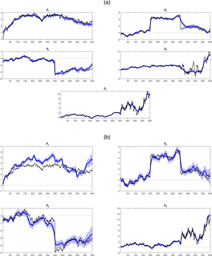
We estimate our proposed framework on two DGPs. For the first case, we estimate our model on the DGP described exactly above, which we denote as the Full-information model. For the second case, we estimate our model on a DGP where the fourth regressor is excluded from the regressor matrix, ${\mathit{X}}_t=(1,{\tilde{x}}_1,{\tilde{x}}_2,0.9{\tilde{x}}_3+z_t)\prime ,$ and all other the DGP assumptions are the same. Therefore, we denote this (omitted variable bias) case as the Limited-information model. Figure 1 plots the posterior median estimates of β_t against the actual DGP simulated parameters. In panel A, it is clearly evident that the estimated β_t parameters of the full-information model track their corresponding simulated DGP parameters very closely and can capture any sudden temporary changes that occur in the data. Panel B plots the estimated β_t parameters of the limited-information model where the fourth regressor is excluded from the model. Similarly, the estimated β_t parameters track their actual counterpart very closely too. For example, the estimated parameter for the fifth regressor, ${\beta }_{5,t},$ displays virtually the same dynamics as their estimated counterpart in the full-information model. Therefore, this highlights that our proposed framework with the Leamer correction can also control for omitted variable bias.

Figure 1. Posterior estimates of the β_t. (a) Panel A: Full-information model and (b) Panel B: Limited-information model.

Notes: The thick blue line is the posterior median of the estimated parameters and the shaded blue area is the associated 68% credible intervals. The black line represents the actual simulated DGP parameters.

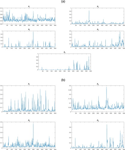
Figure 2 plots the posterior mean of $\mathbb{P}(s_t=1|•)$ for the intercept term in each of the β_t parameters state equation of (29). It is clearly evident that these probabilities peak during the period when a sudden temporary change occurs. For example, in the third regressor, ${\beta }_{3,t},$ a sudden temporary change occurs at $t=350,$ and the associated estimated posterior probability of $\mathbb{P}(s_{3,t}=1|•)$ is close to one at this period of time. Therefore, the posterior mean of $\mathbb{P}(s_t=1|•)$ can also provide us with a probability measure signal of the presence of contagion within the data.

Figure 2. Posterior means estimates of the $\mathbb{P}(s_t=1|•).$ (a) Panel A: Full-information model and (b) Panel B: Limited-information model.

In sum, the simulation study shows that our proposed framework can detect contagion (sudden temporary change) within the data and control for omitted variable bias when an important regressor is excluded from the model.

6. Empirical applications

In this section, we apply the proposed framework to measure contagion and interdependence on two empirical applications: the Chilean foreign exchange market during the Argentine currency in 2001, using the exact dataset from CR, and the recent Covid-19 pandemic on the UK. In Forbes and Rigobon (2000), they define contagion as the “change of shift in the cross-market linkages following a shock in one or more markets,” and interdependence as “a strong association between two markets, both before and after a shock in market.” In terms of our time-varying parameter framework, contagion can be identified as an extreme variation (or temporary change) of the model’s parameters and interdependence between two countries or markets can be characterized either static or dynamic. Coefficients that display smooth time-varying dynamics can be considered as dynamic interdependence where two countries’ markets interaction evolves over time. On the other hand, constant (or time-invariant) coefficients can be interpreted as static interaction between two countries markets over time; we define this as static interdependence. Therefore, based on these two definitions, we can identify dynamic interdependence between two countries or markets by examining the posterior distribution of ω_i. For example, let’s consider a simple example between two countries exchange rates: (30) $$e_{i,t}=\beta e_{j,t}+{\beta }^c{e}_{j,t}+{\omega }_j{\tilde{\beta }}_t{e}_{j,t}+{ϵ}_t,$$(30) where $e_{i,t}$ and $e_{j,t}$ are countries i and j exchange rate respectively. For instance, if the posterior density for ω_j has little mass around zero, this means that there is evidence of time-variation for ${\tilde{\beta }}_t,$ and a high probability of dynamic interdependence between countries’ i and j markets. However, if the posterior density for ω_j has a large mass around zero, this implies no evidence of time-variation for ${\tilde{\beta }}_t,$ and potentially, either static interdependence or contagion could occur between country’s i and j markets.

6.1. Chile Foreign exchange market application

In this section, we replicate the exact empirical application as undertaken by CR, but using our new proposed non-centered parameterization framework. We want to investigate whether our new proposed framework yields similar results as in their paper and provides any additional insights to their results. CR finds two key results from their empirical application. First, they find strong evidence of interdependence between Chile and Brazil and some evidence of contagion from Argentina to Chile. In their empirical application, they use daily financial data from June 2, 1999, to January 31, 2002. For our application, we only focus on their full-information model, which is specified as the following: (31) $$\begin{array}{c}DL{e}_t={\beta }_{0,t}+{\beta }_{1,t}DL{e}_{t-1}+{\beta }_{2,t}{m}_{t-1}+{\beta }_{3,t}D{m}_{t-1}+{\beta }_{4,t}D{i}_{t-1}^{\mathit{CHL}}+{\beta }_{5,t}{s}_{t-1}\\ +{\beta }_{6,t}DL{c}_t+{\beta }_{7,t}DL{b}_t+{\beta }_{8,t}DL{e}_t^{EU}+{\beta }_{9,t}D{i}_t^{AR}+{\beta }_{10,t}D{f}_t^{AR}\\ +{\beta }_{11,t}D{i}_t^{BR}+{\beta }_{12,t}D{f}_t^{BR}+{\beta }_{13,t}DL{e}_t^{BR}+{ϵ}_t,\end{array}$$(31) where D represents the first difference operator, L represents the natural logarithmic transformation and e_t is the Chilean peso/dollar spot exchange rate. There are three types of factors in (31): domestic, regional and global. The domestic factors include Chilean short-term interest rate differential m_t, Chilean long-term interest rate differential $i_t^{\mathit{CHL}}$ and the Chilean stock market differential s_t. The regional factors include: Argentine long-term interest rate differential $i_t^{AR},$ Argentine medium-term interest rate differential $f_t^{AR},$ Brazilian long-term interest rate differential $i_t^{BR},$ Brazilian medium-term interest rate differential $f_t^{BR}$ and Brazilian spot exchange rate $e_t^{BR}.$ Lastly, the global factors include: copper spot price c_t, semiconductors spot price b_t and the Euro spot exchange rate $e_t^{BR}.$ For more details about the data, please see the data appendix of CR.

Equation (31)(31) $$\begin{array}{c}DL{e}_t={\beta }_{0,t}+{\beta }_{1,t}DL{e}_{t-1}+{\beta }_{2,t}{m}_{t-1}+{\beta }_{3,t}D{m}_{t-1}+{\beta }_{4,t}D{i}_{t-1}^{\mathit{CHL}}+{\beta }_{5,t}{s}_{t-1}\\ +{\beta }_{6,t}DL{c}_t+{\beta }_{7,t}DL{b}_t+{\beta }_{8,t}DL{e}_t^{EU}+{\beta }_{9,t}D{i}_t^{AR}+{\beta }_{10,t}D{f}_t^{AR}\\ +{\beta }_{11,t}D{i}_t^{BR}+{\beta }_{12,t}D{f}_t^{BR}+{\beta }_{13,t}DL{e}_t^{BR}+{ϵ}_t,\end{array}$$(31) can rewritten into the non-centered parameterization model of (7) and the findings from our proposed framework are reported in the next subsection.

6.1.1. Empirical results

In this section, we show that our new proposed framework finds no evidence of contagion effects from Argentina or Brazil to Chile. We also illicit three new additional insights that are not captured in CR study. We first examine Figs. 3 and 4, which reports the posterior densities for λ and ν of the two models. We find that most of the posterior mass for λ is centered below 10 and this result is consistent with CR where they also find low values of λ in the full information model. For the degree of freedom parameter ν, majority of the posterior mass are centered above 10, which suggested the SV errors are closed to normality, and there is no evidence fat-tail events presence in the data.

Figure 3. Posterior density for λ.

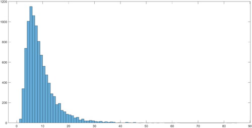
Figure 4. Posterior density for ν.

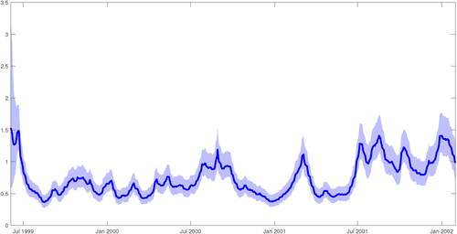
The first key insight we find from our proposed framework, compared to CR, is that the stochastic volatility estimates, reported in Fig. 5, exhibit peaks in their volatility during the Argentine’s economic crisis of late 2001. Also, there are numerous small peaks in the volatility over the sample period. This results highlights the importance of including stochastic volatility in the model as it shows that high-frequency financial data are susceptible to idiosyncratic shocks across time and captures high volatility during periods of crises.

Figure 5. Posterior estimates for $\text{exp}\hspace{0.17em}(h_t/2)$ and the shaded area represents the 68% credible intervals.

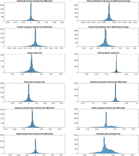
For the second key insight, our new proposed framework allows us to distinguish between static and dynamic interdependence, which CR model cannot. Figure 6 reports the posterior density of ω_i for selected regression coefficients. The majority of the posterior density of ω_i have a large mass centered around zero, which suggest there is no evidence of time-variation and dynamic interdependence. However, the posterior densities of ${\omega }_{D{i}_t^{BR}}$ and ${\omega }_{DL{e}_t^{BR}},$ for the regression coefficients on both the Brazilian long-term interest rate differential and the spot exchange rate, have a large proportion of fat-tail mass. Thus, this suggest there is evidence of time-variation in these parameters, and more importantly, evidence of dynamic interdependence between Chile and Brazil.

Figure 6. The posterior densities of ω_i.

Figure 7 reports the corresponding posterior estimates of the time-varying regression coefficients and it corroborates the findings that we found in the posterior densities in Fig. 6. For example, except for the coefficients on the Brazilian long-term interest rate differential and the Brazilian spot exchange rate, majority of the time-varying regression coefficients are not statistically significant and have no evidence of time-variation as they include zero in their credible intervals. Also, the reported coefficients on the Brazilian long-term interest rate differential and the spot exchange rate display very smooth dynamics over-time and no sudden temporary breaks; this result is consistent with dynamic interdependence definition.

Figure 7. The estimated time-varying regression coefficients. The shaded area represent the 68% credible interva1.

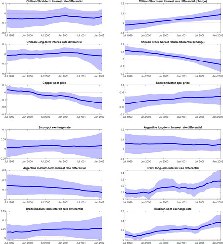
The third key insight we found is that the coefficients on the copper and both the Argentine and Brazilian medium-term interest rate differential, reported in Fig. 7, display smooth time-varying dynamics and in some instance, have their credible interval temporary from zero at a point in time. However, as shown in Fig. 6, the posterior densities of ω_i for these coefficients have large mass centered around zero. Therefore, this suggests that copper and both the Argentine and Brazilian medium-term interest rates play a static interdependent role on the Chilean foreign exchange market.

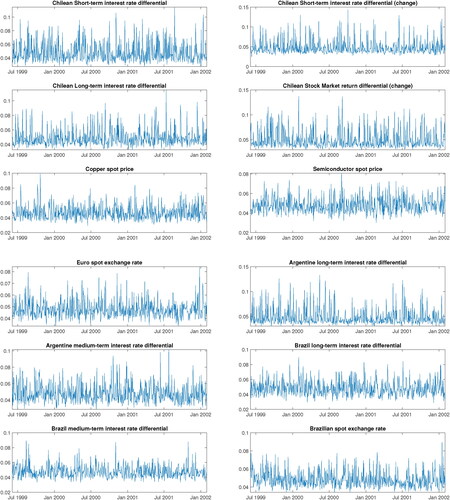
We also report the posterior means of $\mathbb{P}(s_t=1|•)$ for μ_t of the state equation of (29) in Fig. 8, and it is clearly evident there are no pronounce peaks in the posterior probabilities in all the regression coefficients across time. Therefore, we can conclude that is no evidence of contagion effects from Argentine or Brazil to Chile. This result contradicts CR findings where they found some evidence of contagion from Argentina to Chile. The main reason that we found no evidence of contagion effect could be due to our more flexible modeling choice compared to the CR. In CR they assume all the time-varying parameters are driven by one state variance, and this is a very restrictive assumption. In our proposed framework, all the time-varying parameters are driven by their corresponding idiosyncratic state variance, and for majority of the case, we found very little time-variation in all the parameters. Thus, this implies that the restrictive assumption imposed by CR in their model could be overestimating the contagion effect from Argentina to Chile.

Figure 8. Posterior mean estimates of the $\mathbb{P}(s_t=1|•).$

In sum, our proposed new framework finds no evidence of contagion effect from Argentina or Brazil to Chile, which contradicts the findings of CR. We also found three key additional insights using our proposed framework compared to CR. First, we found that the inclusion of the stochastic volatility in the model is important as it captures the high volatility during periods of crises. Second, we found evidence that the interdependence between Chile and Brazil are dynamic. Lastly, we found evidence of static interdependence between Chile and copper, and both the Argentine and Brazilian medium-term interest rates.

6.2. Covid-19 pandemic in the United Kingdom

In this section, we apply our proposed framework to investigate the recent Covid-19 pandemic in the UK. Specifically, we model the relationship of (32) $$\begin{array}{c}\mathit{COVID}{19}_t^{UK}={\beta }_{1t}+{\beta }_{2t}C\mathit{OVID}{19}_t^{\mathit{ITA}}+{\beta }_{3t}C\mathit{OVID}{19}_t^{\mathit{GER}}+{\beta }_{4t}C\mathit{OVID}{19}_t^{\mathit{FRA}}+{\beta }_{5t}C\mathit{OVID}{19}_t^{\mathit{ESP}}\\ +{\beta }_{6t}C\mathit{OVID}{19}_t^{\mathit{POL}}+{\beta }_{7t}C\mathit{OVID}{19}_t^{\mathit{POR}}+{\beta }_{8t}C\mathit{OVID}{19}_t^{\mathit{SWE}}+{ϵ}_t,\end{array}$$(32) where $\mathit{COVID}{19}_t^i$ is the i – th country’s growth rate of the cumulative number of confirmed cases given in a day. We follow Ding et al. (2021), and calculate the growth rate of the cumulative number of confirmed cases as $\text{ln}\hspace{0.17em}(1+\mathit{Cumulative} \mathit{Case}{s}_t^i)-\hspace{0.17em}\text{ln}\hspace{0.17em}(1+\mathit{Cumulative} \mathit{Case}{s}_{t-1}^i).$ For our regressors, we consider seven European countries that have close ties with the UK. They are Italy, Germany, France, Spain, Poland, Portugal and Sweden. We use daily data gathered from the John Hopkins University Covid-19 database, and it spans from June 2, 2020, to September 22, 2021.

6.2.1. Empirical results

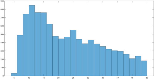
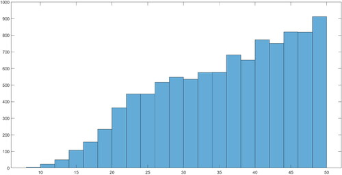
We first plot the posterior densities of λ and ν in Figs. 9 and 10, respectively. The posterior median of λ is about 23, and the associated 68% credible interval is between 13 and 45. This relatively high number for λ is not surprising given that we have only included seven European countries in our model. Therefore, the Leamer correction within our proposed framework is correcting for this omitted variable bias. Lastly, the posterior median for ν is about 37, which suggest that the SV errors are close to normality, and there is no evidence of fat-tails event presence in Covid-19 data.

Figure 9. Posterior density for λ.

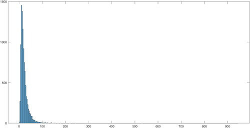
Figure 10. Posterior density for ν.

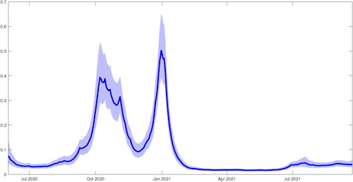
Figure 11 plots the posterior estimates of the stochastic volatility. It is evident that the peaks in the volatility appear to occur during the second wave of the Covid-19 pandemic in the UK. The first peak in volatility during October 2020 could result from the UK government easing restrictions in August 2020, while the second peak in volatility during January 2021 is likely driven by the rapid spread of the new alpha (or Kent) variant in December 2020. This result indicates that discovering a new Covid-19 variant strain seems to induce a high uncertainty level within Covid-19 cases. In other words, shocks to Covid-19 cases are more pronounced during the emergence of a new strain.

Figure 11. Posterior estimates for $\text{exp}\hspace{0.17em}(h_t/2)$ and the shaded area represents the 68% credible intervals.

We plot the posterior densities of ω_i for all the regression coefficients in Fig. 12. Except for Italy, all the six European countries have a large portion of non-zero mass within their posterior density. Thus, there is clear evidence of time-variation within these country’s coefficients. To investigate further, we plot the corresponding posterior estimates of the time-varying regression coefficients in Fig. 13, which corroborates the findings in Fig. 12. Therefore, we can conclude that there is evidence of dynamic interdependence of Covid-19 cases between the UK and these six European countries, given that majority of each country’s coefficient displays smooth time-varying dynamics. These results seem to suggest that border restrictions enforced by the UK government were largely ineffective in preventing the importation of Covid-19 cases from these six European countries, and the mandatory hotel quarantine policy should have been implemented earlier in the first wave of the Covid-19 pandemic.

Figure 12. The posterior densities of ω_i.

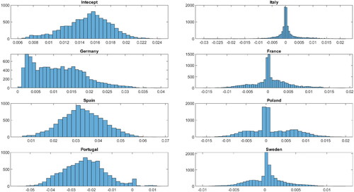
Figure 13. The estimated time-varying regression coefficients. The shaded area represent the 68% credible interva1.

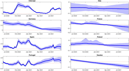
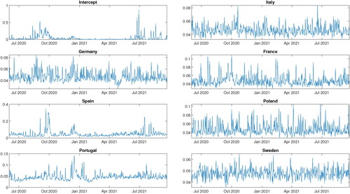
From Fig. 13, both Spain and Portugal display a sudden temporary change in their coefficients during October 2020 and January 2021, respectively. We report the posterior means of $\mathbb{P}(s_t=1|•)$ for μ_t of the state equation of (29) in Fig. 14. We can see that the posterior probabilities of these two countries do indeed peak at these two dates. Therefore, we can conclude that there may be evidence of contagion effects of Covid-19 cases from both Spain and Portugal to the UK. This result is highly plausible given that both Spain and Portugal are highly popular tourist destinations for UK travelers.

Figure 14. Posterior mean estimates of the $\mathbb{P}(s_t=1|•).$

7. Conclusion

We have developed a flexible Bayesian time-varying parameter model with Leamer correction within a non-centered parameterization framework to measure contagion and interdependence. The simulation study shows that our new proposed framework can detect contagion and correct the omitted variable bias when a significant regressor is excluded from the model. We apply our new proposed framework to two empirical applications: the Chilean foreign exchange market during the Argentine crisis in 2001 and the recent Covid-19 pandemic in the UK. We found that our new proposed framework finds no evidence of contagion effects from Argentina or Brazil to Chile, which contradicts the findings of CR. In addition, we found three additional key insights compared to CR.

Regarding the Covid-19 pandemic in the UK, using our proposed framework, we found evidence that the UK government was largely ineffective in preventing the importation of Covid-19 cases from abroad, and there is evidence of contagion effects of Covid-19 cases from both Spain and Portugal, which are highly popular tourist destinations for UK travelers. For future work, it would be interesting to extend the non-centered parameterization framework with Leamer correction to a VAR framework and apply it to macroeconomic applications, such as inflation modeling.

Acknowledgments

We thank Matteo Ciccarelli for sharing his dataset for the Chilean application. We thank Joshua Chan, Jamie Cross and Gary Koop for their comments on an earlier version of the draft.

Appendix

A.1 Model specification

To implement Step 4, let us first define $T_1={\sum }_{t=1}^T\mathbf{1}(s_t=1)$ and $T_2=T-T_1.$ Next, it is easy show that when s_t = 1, the conditional posterior for ${\mu }_t={\tilde{\mu }}_1$ is $$({\tilde{\mu }}_1|•)\sim N({\widehat{\mu }}_1,{\mathit{K}}_{{\mu }_1}),$$ where ${\mathit{K}}_{{\mu }_1}={(X_{{\mu }_1}^{\prime }{X}_{{\mu }_1}+V_{{\mu }_1}^{-1})}^{-1}$ and ${\widehat{\mu }}_1={\mathit{K}}_{{\mu }_1}(X_{{\mu }_1}^{\prime }△{\tilde{\beta }}_t+V_{{\mu }_1}^{-1}{\overline{\mu }}_1).$ Note here $X_{{\mu }_1}$ is a $T_1\times 1$ column vector of ones, and $△{\tilde{\beta }}_t=({\tilde{\beta }}_0-{\tilde{\beta }}_1,\dots ,{\tilde{\beta }}_{T-1}-{\tilde{\beta }}_T)\prime .$ A similar logic is also applied to derive the conditional posterior of $({\tilde{\mu }}_2|•)$ when s_t = 2.

To implement Step 5, it is straightforward to show that $$\mathbb{P}(s_t=1|•)=\frac{N(△{\tilde{\beta }}_t,{\tilde{\mu }}_1,1)q}{N(△{\tilde{\beta }}_t,{\tilde{\mu }}_1,1)q+N(△{\tilde{\beta }}_t,{\tilde{\mu }}_2,1)(1-q)},$$

Thus, $$\mathbb{P}(s_t=2|•)=1-\mathbb{P}(s_t=1|•).$$

We simulate s_t with a success probability $q_t=\mathbb{P}(s_t=1|•),$ we first obtain a draw from standard uniform distribution, $u\sim U(0,1).$ If $u<q_t,$ then we set s_t = 1; otherwise we set s_t = 2. Finally for Step 6, the conditional posterior for $(q|•)\sim B(a_0+T_1,b_0+T_2).$

To implement Step 7, we first transform the model (7) to be $\tilde{\mathit{y}}={\Delta }^{-\frac{1}{2}}(\mathit{y}-\mathit{X}\beta -\mathit{X}{\beta }^c-\mathit{Z}\tilde{\beta }),$ where ${\Delta }^{-\frac{1}{2}}=\text{diag}({\delta }_1^{-\frac{1}{2}},\dots ,{\delta }_T^{-\frac{1}{2}}).$ Then, $$(\tilde{\mathit{y}}|•)\sim N(0,{\mathit{S}}_{\mathit{y}}),$$ where ${\mathit{S}}_{\mathit{y}}=\text{diag}(e^{h_1},\dots ,e^{h_T}).$ Therefore, we can directly apply the Kim et al. (1998) auxiliary mixture sampler with precision based methods, as described in Chan and Hsiao (2014), to simulate $(\mathit{h}|•).$

To implement Step 8, since ${\delta }_1.\dots ,{\delta }_T$ are conditionally independent given the model parameters and the data, we can sample each of them sequentially. In fact, we have: $$({\delta }_t|•)\sim IG(\frac{\nu +1}{2},\frac{\nu +{(y_t-{\mathit{x}}_t\beta -{\mathit{x}}_t{\beta }^c-{\mathit{x}}_t\Omega {\tilde{\beta }}_t)}^2}{2}),$$

To implement Step 9, we follow the methodology govern in Chan and Hsiao (2014). To draw the degree of freedom parameter ν, we first derive the log-density log $p(\nu |\delta )$ from (15) and the prior assumption of (16), where (33) $$\text{log}\hspace{0.17em}(\nu |\delta )\propto \frac{T\nu }{2}\text{log}\hspace{0.17em}(\nu /2)-T\hspace{0.17em}\text{log}\hspace{0.17em}\Gamma (\nu /2)-(\frac{\nu }{2}+1)\sum _{t=1}^T\hspace{0.17em}\text{log}\hspace{0.17em}{\delta }_t-0.5\sum _{t=1}^T{\delta }_t^{-1}+c,$$(33) where $0<\nu <\overline{\nu }$ and c is normalizing constant. It is easy to check that the first and second derivatives of the log-density with respect to ν are given by (34) $$\frac{d\hspace{0.17em}\text{log}\hspace{0.17em}(\nu |\mathit{\delta })}{d\nu }=\frac{T}{2}\text{log}\hspace{0.17em}(\nu /2)-\frac{T}{2}-\frac{T}{2}\Psi (\nu /2)-0.5\sum _{t=1}^T\hspace{0.17em}\text{log}\hspace{0.17em}{\delta }_t-0.5\sum _{t=1}^T{\delta }_t^{-1},$$(34) (35) $$\frac{d^2\hspace{0.17em}\text{log}\hspace{0.17em}(\nu |\mathit{\delta })}{d{\nu }^2}=\frac{T}{2\nu }-\frac{T}{4}\Psi \prime (\nu /2),$$(35) where $\Psi (x)=\frac{d}{dx}\text{log}\hspace{0.17em}\Gamma (x)$ and $\Psi \prime (x)=\frac{d}{dx}\Psi (x)$ are respectively the digamma and trigamma functions. Since first and second derivatives can be evaluated quickly, we can maximize the log $p(\nu |\mathit{\delta })$ using the Newton-Raphson method and obtain the mode and the negative hessian evaluated at the mode, denoted $\widehat{\nu }$ and $K_{\nu },$ respectively. Then, we implement an independence chain Metropolis-Hastings step with a proposal distribution of $N(\widehat{\nu },K_{\nu }^{-1}).$

Lastly, to implement Step 10, except for $(\rho |•),$ all the conditional posteriors are standard and straightforward: $$({\sigma }_h^2|•)\sim IG({\alpha }_h+\frac{T}{2},S_h+\frac{\sum _{t=1}^T{(h_t-{\mu }_h-\rho h_{t-1})}^2}{2}),$$ $$({\mu }_h|•)\sim N(\widehat{{\mu }_h},D_{\mu }),$$ where $D_{\mu }={(V_{{\mu }_h}^{-1}+\frac{X_{\mu }^{\prime }{X}_{\mu }}{{\sigma }_h^2})}^{-1},$ $\widehat{{\mu }_h}=D_{\mu }(V_{{\mu }_h}^{-1}{\mu }_0+\frac{X_{\mu }^{\prime }{z}_{\mu }}{{\sigma }_h^2}),$ $X_{\mu }=(1,\dots ,1)\prime$ is a $T\times 1$ vector and $z_{\mu }=(h_1-\rho h_0,h_2-\rho h_1,\dots ,h_t-\rho h_{t-1})\prime .$ $$(h_0|•)\sim N({\widehat{h}}_0,D_{h_0}),$$ where $D_{h_0}={(\frac{{\rho }^2}{{\sigma }_h^2}+\frac{(1-\rho )}{{\sigma }_h^2})}^{-1}$ and ${\widehat{h}}_0=D_{h_0}\left(\frac{h_1-{\mu }_h}{{\sigma }_h^2}\right).$ $$({\tilde{\beta }}_0|•)\sim N(\widehat{{\tilde{\beta }}_0},D_{{\tilde{\beta }}_0}),$$ where $D_{{\tilde{\beta }}_0}={({(\lambda V_{\mathit{OLS}})}^{-1}+{\mathit{I}}_k)}^{-1}$ and $\widehat{{\tilde{\beta }}_0}=D_{{\tilde{\beta }}_0}{\tilde{\beta }}_1.$

To simulate $(\rho |•),$ we follow Chan and Hsiao (2014) and use a Metropolis-Hastings step to draw ρ: (36) $$p(\rho |•)\propto p(\rho )g(\rho )\hspace{0.17em}\text{exp}\hspace{0.17em}-\frac{1}{2{\sigma }_h^2}\sum _{t=1}^T{(h_t-{\mu }_h-\rho h_{t-1})}^2,$$(36) where $g(\rho )={(1-{\rho }^2)}^{\frac{1}{2}}\hspace{0.17em}\text{exp}\hspace{0.17em}(-\frac{1}{2{\sigma }_h^2}(1-{\rho }^2)h_0^2)$ and $p(\rho )$ is the truncated normal given in section 3 of the article.

References

- Caporin, M., Pelizzon, L., Ravazzolo, F., Rigobon, R. (2018). Measuring sovereign contagion in Europe. Journal of Financial Stability 34:150–181. doi:https://doi.org/10.1016/j.jfs.2017.12.004
- Carriero, A., Clark, T. E., Marcellino, M. G., & Mertens, E. (2021). Addressing COVID-19 outliers in BVARs with stochastic volatility. Federal Reserve of Cleveland Working Paper.
- Chan, J. C. (2019). Large hybrid time-varying parameter VARs. Manuscript.
- Chan, J. C. (2020). Large Bayesian VARs: a flexible Kronecker error covariance structure. Journal of Business and Economic Statistics 38(1):68–79. doi:https://doi.org/10.1080/07350015.2018.1451336
- Chan, J. C., Eisenstat, E. (2018). Bayesian model comparison for time-varying parameter VARs with stochastic volatility. Journal of Applied Econometrics 33(4):509–532. doi:https://doi.org/10.1002/jae.2617
- Chan, J. C., Eisenstat, E., Strachan, R. W. (2020). Reducing the state space dimension in a large TVP-VAR. Journal of Econometrics 218(1):105–118. doi:https://doi.org/10.1016/j.jeconom.2019.11.006
- Chan, J., Hsiao, C. (2014). Estimation of stochastic volatility models with heavy tails and serial dependence. In: Jeliazkov I., Yang, X.-S., eds., Bayesian Inference in the Social Sciences, Hoboken, NJ: John Wiley & Sons, pp. 159–180.
- Chan, J., Jeliazkov, I. (2009). Efficient simulation and integrated likelihood estimation in state space models. International Journal of Mathematical Modelling and Numerical Optimisation 1(1/2):101–120. doi:https://doi.org/10.1504/IJMMNO.2009.030090
- Ciccarelli, M., Rebucci, A. (2006). Measuring contagion and interdependence with a bayesian time-varying coefficient model: an application to the chilean FX market during the argentine crisis. Journal of Financial Econometrics 5(2):285–320. doi:https://doi.org/10.1093/jjfinec/nbm003
- Clark, T. E., Ravazzolo, F. (2015). Macroeconomic forecasting performance under alternative specifications of time-varying volatility. Journal of Applied Econometrics 30(4):551–575. doi:https://doi.org/10.1002/jae.2379
- Cross, J., Poon, A. (2016). Forecasting structural change and fat-tailed events in australian macroeconomic variables. Economic Modelling 58:34–51. doi:https://doi.org/10.1016/j.econmod.2016.04.021
- Ding, W., Levine, R., Lin, C., Xie, W. (2021). Corporate immunity to the COVID-19 pandemic. Journal of Financial Economics 141(2):802–830. doi:https://doi.org/10.1016/j.jfineco.2021.03.005
- Dungey, M., Fry, R., González-Hermosillo, B., Martin, V. L. (2005). Empirical modelling of contagion: a review of methodologies. Quantitative finance 5(1):9–24. doi:https://doi.org/10.1080/14697680500142045
- Forbes, K., Rigobon, R. (2000). Contagion in latin america: Definitions, measurement, and policy implications. Economïoea Journal 1(2):1–46.
- Frühwirth-Schnatter, S., Wagner, H. (2010). Stochastic model specification search for gaussian and partial non-Gaussian state space models. Journal of Econometrics 154(1):85–100. doi:https://doi.org/10.1016/j.jeconom.2009.07.003
- Grubel, H. G., Fadner, K. (1971). The interdependence of international equity markets. The Journal of Finance 26(1):89–94. doi:https://doi.org/10.1111/j.1540-6261.1971.tb00591.x
- Guidolin, M., Hansen, E., Pedio, M. (2019). Cross-asset contagion in the financial crisis: a bayesian time-varying parameter approach. Journal of Financial Markets 45:83–114. doi:https://doi.org/10.1016/j.finmar.2019.04.001
- Huber, F., Koop, G., Onorante, L. (2021). Inducing sparsity and shrinkage in time-varying parameter models. Journal of Business and Economic Statistics 39(3):669–683. doi:https://doi.org/10.1080/07350015.2020.1713796
- Kim, S., Shepherd, N., Chib, S. (1998). Stochastic volatility: Likelihood inference and comparison with ARCH models. Review of Economic Studies 65(3):361–393. doi:https://doi.org/10.1111/1467-937X.00050
- Leamer, E. E., Leamer, E. E. (1978). Specification Searches: Ad Hoc Inference with Nonexperimental Data (Vol. 53). New York: Wiley.
- Ngiam, K. J. (2000). Coping with the Asian Financial Crisis: The Singapore Experience. From crisis to recovery: East Asia rising again.
- Rigobon, R. (2002). Contagion: how to measure it? In: Preventing Currency Crises in Emerging Markets. Chicago: University of Chicago Press, pp. 269–334.
- Sharpe, W. F. (1964). Capital asset prices: a theory of market equilibrium under conditions of risk. The Journal of Finance 19(3):425–442.