Selecting the number of factors in approximate factor models using group variable regularization

Abstract.

We propose a novel method for the estimation of the number of factors in approximate factor models. The model is based on a penalized maximum likelihood approach incorporating an adaptive hierarchical lasso penalty function that enables setting entire columns of the factor loadings matrix to zero, which corresponds to removing uninformative factors. Additionally, the model is capable of estimating weak factors by allowing for sparsity in the non zero columns. We prove that the proposed estimator consistently estimates the true number of factors. Simulation experiments reveal superior selection accuracies for our method in finite samples over existing approaches, especially for data with cross-sectional and serial correlations. In an empirical application on a large macroeconomic dataset, we show that the mean squared forecast errors of an approximate factor model are lower if the number of included factors is selected by our method.

Keywords:

• Adaptive hierarchical lasso
• approximate factor model
• number of factors
• weak factors

JEL classification::

• C32
• C38
• C52

1. Introduction

In the recent years, high-dimensional factor models have become very popular in finance and macroeconomics. Factor models are used to concentrate the information contained in a large number of economic variables into a substantially smaller number of latent factors. The economic relevance of factor models has been shown in several macroeconomic and financial applications that consider business cycle analysis (Forni and Reichlin 1998; Giannone, Reichlin, and Sala 2002), forecasting of large-dimensional datasets (Stock and Watson 2002, 2005), structural analysis based on factor-augmented vector autoregressive models (FAVAR) (Bernanke, Boivin, and Eliasz 2005; Stock and Watson 2016), or the estimation of large dimensional covariance matrices (Fan, Fan, and Lv 2008; Fan, Liao, and Mincheva 2013). To avoid a misspecification of the factor model, it is crucial to use the true number of factors, which has to be determined a priori. Using the correct number of factors is of practical relevance as well. For instance, in the FAVAR model, it is important to include the true number of factors so that the entire space spanned by the structural shocks is estimated consistently and the policy recommendations inferred from the FAVAR model are reliable.

In this article, we introduce a novel method for selecting the number of factors in approximate factor models and provide new insights to the extensive research conducted in this field. Our adaptive hierarchical factor model (AHFM) can be classified into selection procedures that rely on regularization methods. The AHFM refers to a penalized maximum likelihood approach where we use an adaptive hierarchical lasso penalty function, introduced by Zhou and Zhu (2010) that allows for a penalization of the factor loadings matrix. The beneficial features of the adaptive hierarchical lasso penalty function lie in its ability to set entire columns in the factor loadings matrix to zero, which corresponds to removing uninformative factors. In order to obtain an estimate for the number of factors, our approach focuses on the non zero columns of the estimated factor loadings matrix.

Additionally, the adaptive hierarchical lasso penalty introduces sparsity in the non zero columns of the factor loadings matrix. The sparsity in the relevant groups allows for the estimation of weak factors, which only affect a subset of the observed variables. Thus, the AHFM framework enables the distinction between pervasive and weak factors, relaxes the pervasiveness assumption conventionally made in the standard approximate factor model (see e.g., Bai and Ng 2002; Stock and Watson 2002), and improves the factor identification. The pervasiveness assumption, implies a clear separation of the diverging eigenvalues corresponding to the common component and the bounded eigenvalues of the covariance matrix of the idiosyncratic errors. However, such a separation is typically not found in practice (see e.g., Daniele, Pohlmeier, and Zagidullina 2020). Hence, by allowing for slower divergence rates in the common component, the weak factor framework is more appropriate for modeling real datasets. Another important reason for considering weakly influential factors, is a potential increase in the estimation error, if those are not taken into account in the factor modeling framework. In fact, static factors, which are actually weak, are estimated with large errors if the principal component analysis (PCA) method is used, as shown by Onatski (2012). The empirical importance of the weak factor framework is supported by various research studies. In the context of macroeconomic forecasting, Boivin and Ng (2006) show that the performance of the PCA estimator deteriorates as more uninformative series are added to the panel. These time series are not affected by the strong factors that drive the common fluctuations in output or prices and, thus, are better modeled in the weak factor framework. In the arbitrage pricing theory (Ross 1976), the weak factor assumption implies factors of different strengths that affect a decreasing fraction of the asset returns. This supports the empirical evidence that the eigenvalues of the sample covariance matrix of asset returns diverge at different rates that are slower than the number of variables N (see e.g., Trzcinka 1986). Recently, Uematsu and Yamagata (2022) introduced an approach for estimating weakly influential factors in the principal component analysis setting, by using the possible sparse structure in the factor loadings matrix.

A variety of methods have been proposed in the literature for determining the number of factors. Bai and Ng (2002) propose different selection criteria that are modifications of the standard Bayesian information criterion to consistently estimate the number of factors in large dimensional datasets. Onatski (2010) shows that the largest bounded eigenvalues of the sample covariance matrix cluster around a single point and proposes an estimator that consistently separates these eigenvalues, from the diverging eigenvalues that result in the number of selected factors. Ahn and Horenstein (2013) propose two estimators for the number of factors that rely on the ratio of adjacent eigenvalues of the sample covariance matrix of the data. The estimators offer good selection rates in the case of cross-sectionally and serially correlated data as well. More recently, the research is also focusing on regularization methods for selecting the number of factors. Caner and Han (2014) introduce a penalized least squares optimization method that relies on a group bridge penalty function and allows for setting entire columns of the factor loadings matrix to zero. The authors focus on the number of non zero columns as an estimate for the true number of factors. Freyaldenhoven (2022) introduces a new class of estimators to determine the number of factors in a framework that incorporates local factors affecting only a subset of the observed variables.

In order to consistently estimate the number of factors, common selection methods require a clear separation of the diverging and bounded eigenvalues in the data covariance matrix. However, a clear separation of the two sets of eigenvalues is no longer present if the idiosyncratic component contains a non trivial amount of correlation, as we point out in the simulation study. Especially, for correlated data, the existing methods tend to provide estimates for the number of factors that deviate from the true quantity. In contrast to that, our AHFM, which is based on the weak factor framework, allows for considerably slower divergence rates in the eigenvalues of the common component. Hence, the AHFM is able to measure more narrow distances between the diverging and bounded eigenvalues and its selection accuracy is less sensitive to correlations in the idiosyncratic component.

In the theoretical part of the article, we show that the factor loadings of the relevant factors based on our method are consistently estimated under the average Frobenius norm. At the same time, the AHFM shrinks the factor loadings of the uninformative factors toward zero with probability tending to one. Hence, our method consistently estimates the true number of factors.

In our Monte Carlo studies, we analyze the finite sample selection accuracy of our method and compare it to methods that are commonly used in the literature. The simulation results reveal that our method offers accurate selection rates for the true number of factors in small samples and shows, particularly for datasets with cross-sectional and temporal correlations, more precise results compared to the competing approaches in most of the cases. Especially, for correlated data, we notice that the selection approach by Bai and Ng (2002) tends to overestimate the true number of factors. Furthermore, our adaptive hierarchical factor model detects the correct number of factors in almost all cases, as both the temporal dimension T and cross-sectional dimension N tend to infinity. In a second simulation study that incorporates weak factors in the data generating process, we observe that the AHFM model typically deviates less often from the true number of factors compared to the competing methods and converges faster to the true quantity as N and T increase. In an empirical application, we determine the number of factors in a large dimensional dataset based on the FRED-MD database by McCracken and Ng (2016) and focus on an out-of-sample forecasting experiment of macroeconomic variables. The results show that the forecasting accuracy of an approximate factor model is improved if the number of included factors is selected by our adaptive hierarchical factor model.

The remainder of this article is organized as follows. In Section 2, we introduce the econometric framework of the proposed selection method for the number of factors. Section 3 introduces the model assumptions and the theoretical results. The implementation details are discussed in Section 4. In Section 5, we discuss the simulation studies and investigate the finite sample selection accuracy of our method, while Section 6 provides an empirical example on determining the number of factors in a large dimensional macroeconomic dataset and forecasting key macroeconomic variables. Finally, the article concludes in Section 7.

Throughout the article, we will use the following notation: π_max(A) and π_min(A) are the maximum and minimum eigenvalue of a matrix A. Further, $\Vert A\Vert$ and ${\Vert A\Vert }_F$ denote the spectral and Frobenius norm of A, respectively. They are defined as $\Vert A\Vert =\sqrt{{\pi }_{max}(A^{\prime }A)}$ and ${\Vert A\Vert }_F=\sqrt{\text{tr}\left(A^{\prime }A\right)}$. For the non random sequences x_N and a_N, with $N=1,2,\dots$, we use the notation x_N = 𝒪(1), if x_N is uniformly bounded in N, i.e., there exists a constant M < ∞ such that $|x_N|\le M$ for all N. x_N = 𝒪(a_N), if $a_N^{-1}{x}_N=\mathcal{O}(1)$. Moreover, x_N = o(a_N), if $a_N^{-1}{x}_N\to 0$, for N→∞. Similarly, for a random sequence z_N, we say z_N = 𝒪_p(1), if z_N is bounded in probability, i.e., for any ε > 0 there is a constant M_ε < ∞ such that $\underset{N\to \mathrm{\infty }}{limsup}\mathbb{P}(|z_N|>M_{\epsilon })\le \epsilon$. Moreover, z_N = 𝒪_p(a_N), if $a_N^{-1}{z}_N={\mathcal{O}}_p(1)$ and z_N = o_p(a_N), if $a_N^{-1}{z}_N\stackrel{p}{\to }0$, for N→∞. For the sequences a_N and b_N, we write a_N≍b_N, if a_N = 𝒪(b_N) and b_N = 𝒪(a_N).

2. Factor model for the estimation of the number of factors

We start with introducing the approximate factor model (AFM) framework proposed by Chamberlain and Rothschild (1983), which is defined as (2.1) $$\begin{array}{l}{x}_{it}={\lambda }_{i,0}^{\prime }{f}_{t,0}+u_{it},\end{array}$$(2.1) where x_it is the observed data for the i-th variable at time t, for $i=1,\dots ,N$ and $t=1,\dots ,T$, such that N and T denote the sample size in the cross-section and time dimension, respectively. We concentrate on large dimensional factor models, where both N and T diverge to infinity. The time series x_it are assumed to be weakly stationary, demeaned, and standardized. λ_{i, 0} is a (r×1)-dimensional vector of unobserved factor loadings for variable i and f_{t, 0} is the corresponding (r×1)-dimensional vector of latent factors at time t. The true number of factors is defined as r. Finally, u_it denotes the idiosyncratic component. As we refer to the AFM framework, u_it incorporates some weak temporal and cross-sectional correlations. Hence, the AFM offers a generalization of the strict factor model that assumes uncorrelated idiosyncratic errors. The matrix representation of Eq. (2.1(2.1) $$\begin{array}{l}{x}_{it}={\lambda }_{i,0}^{\prime }{f}_{t,0}+u_{it},\end{array}$$(2.1) ) is given by (2.2) $$\begin{array}{l}X=F_0{\mathrm{\Lambda }}_0^{\prime }+u\end{array}$$(2.2) where X denotes a (T×N) matrix of observed data. $F_0=(f_{1,0},\dots ,f_{T,0}{)}^{\prime }$ is a (T×r)-dimensional matrix of factors, ${\mathrm{\Lambda }}_0=({\lambda }_{1,0},\dots ,{\lambda }_{N,0}{)}^{\prime }$ is a (N×r) matrix of corresponding factor loadings, and u is a (T×N)-dimensional matrix of the idiosyncratic errors with covariance matrix Σ_u0.

2.1. Hierarchical factor model

In order to estimate the approximate factor model in (2.2(2.2) $$\begin{array}{l}X=F_0{\mathrm{\Lambda }}_0^{\prime }+u\end{array}$$(2.2) ), we refer to the quasi maximum likelihood (QML) approach, which is discussed in e.g., Bai and Li (2016). The negative log-likelihood function for the covariance matrix of the data in the approximate factor model is defined as (2.3) $$\begin{array}{l}\mathcal{L}(\mathrm{\Lambda },{\mathrm{\Sigma }}_F,{\mathrm{\Sigma }}_u)=\frac{1}{N}\log |\mathrm{\Lambda }{\mathrm{\Sigma }}_F{\mathrm{\Lambda }}^{\prime }+{\mathrm{\Sigma }}_u|+\frac{1}{N}\text{tr}\left[S_x{(\mathrm{\Lambda }{\mathrm{\Sigma }}_F{\mathrm{\Lambda }}^{\prime }+{\mathrm{\Sigma }}_u)}^{-1}\right],\end{array}$$(2.3) where $S_x=1/T{\sum }_{t=1}^T{x}_t{x}_t^{\prime }$ denotes the sample covariance matrix of the observed data, Λ is a (N×p)-dimensional factor loadings matrix, with p corresponding to a predetermined upper bound on the number of included factors, such that p≥r and Σ_F is a low dimensional covariance matrix of the factors. As Σ_u incorporates correlations of general form, the number of free parameters in Σ_u is potentially of order 𝒪(N²). Hence, the joint estimation of the entire set of variables in (2.3(2.3) $$\begin{array}{l}\mathcal{L}(\mathrm{\Lambda },{\mathrm{\Sigma }}_F,{\mathrm{\Sigma }}_u)=\frac{1}{N}\log |\mathrm{\Lambda }{\mathrm{\Sigma }}_F{\mathrm{\Lambda }}^{\prime }+{\mathrm{\Sigma }}_u|+\frac{1}{N}\text{tr}\left[S_x{(\mathrm{\Lambda }{\mathrm{\Sigma }}_F{\mathrm{\Lambda }}^{\prime }+{\mathrm{\Sigma }}_u)}^{-1}\right],\end{array}$$(2.3) ) is intractable without any regularization on Σ_u, as the number of parameters in the model may exceed the number of available observations T. In order to mitigate this problem, we adopt the idiosyncratic error structure of a strict factor model in the first step of our model estimation. More specifically, we treat Σ_u as a diagonal matrix and define Φ_u = diag(Σ_u) as a diagonal matrix incorporating only the elements of the main diagonal of Σ_u. Furthermore, the covariance of the factors is restricted to Σ_F = I_p. Based on the diagonality assumption on Σ_u and the restriction on Σ_F, the objective function reduces to (2.4) $$\begin{array}{l}\mathcal{L}(\mathrm{\Lambda },{\mathrm{\Phi }}_u)=\frac{1}{N}\log |\mathrm{\Lambda }{\mathrm{\Lambda }}^{\prime }+{\mathrm{\Phi }}_u|+\frac{1}{N}\text{tr}\left[S_x{(\mathrm{\Lambda }{\mathrm{\Lambda }}^{\prime }+{\mathrm{\Phi }}_u)}^{-1}\right].\end{array}$$(2.4)

Similar to Bai and Li (2016), Eq. (2.4(2.4) $$\begin{array}{l}\mathcal{L}(\mathrm{\Lambda },{\mathrm{\Phi }}_u)=\frac{1}{N}\log |\mathrm{\Lambda }{\mathrm{\Lambda }}^{\prime }+{\mathrm{\Phi }}_u|+\frac{1}{N}\text{tr}\left[S_x{(\mathrm{\Lambda }{\mathrm{\Lambda }}^{\prime }+{\mathrm{\Phi }}_u)}^{-1}\right].\end{array}$$(2.4) ) should be regarded as a quasi log-likelihood function, as it neglects the general form of correlations in the idiosyncratic errors. Nevertheless, in Section 3 we show that the quasi maximum likelihood estimator based on (2.4(2.4) $$\begin{array}{l}\mathcal{L}(\mathrm{\Lambda },{\mathrm{\Phi }}_u)=\frac{1}{N}\log |\mathrm{\Lambda }{\mathrm{\Lambda }}^{\prime }+{\mathrm{\Phi }}_u|+\frac{1}{N}\text{tr}\left[S_x{(\mathrm{\Lambda }{\mathrm{\Lambda }}^{\prime }+{\mathrm{\Phi }}_u)}^{-1}\right].\end{array}$$(2.4) ) is consistent.

In the following, we introduce our hierarchical factor model (HFM) for the estimation of the number of factors in the AFM. The hierarchical factor model is based on a penalized ML approach and augments the quasi log-likelihood function in (2.4(2.4) $$\begin{array}{l}\mathcal{L}(\mathrm{\Lambda },{\mathrm{\Phi }}_u)=\frac{1}{N}\log |\mathrm{\Lambda }{\mathrm{\Lambda }}^{\prime }+{\mathrm{\Phi }}_u|+\frac{1}{N}\text{tr}\left[S_x{(\mathrm{\Lambda }{\mathrm{\Lambda }}^{\prime }+{\mathrm{\Phi }}_u)}^{-1}\right].\end{array}$$(2.4) ) with the hierarchical lasso penalty function introduced by Zhou and Zhu (2010). This penalty allows for group selection and additionally introduces sparsity in the selected groups. In our setting, the different columns in Λ are referred as factor groups. Hence, the hierarchical lasso penalty is able to set entire columns of Λ to zero, which is equivalent to disregarding the corresponding factor.

More specifically, we solve the following augmented optimization problem (2.5) $$\begin{array}{l}\underset{\mathrm{\Lambda },{\mathrm{\Phi }}_u}{min}[\mathcal{L}(\mathrm{\Lambda },{\mathrm{\Phi }}_u)+\frac{\mu }{N}\sum _{k=1}^p\sqrt{\sum _{i=1}^N\left|{\lambda }_i^{(k)}\right|}],\end{array}$$(2.5) where ${\lambda }_i^{(k)}$ corresponds to the i-th factor loading of the k-th latent factor and μ represents a regularization parameter that controls the strength of penalization. The penalty function in (2.5(2.5) $$\begin{array}{l}\underset{\mathrm{\Lambda },{\mathrm{\Phi }}_u}{min}[\mathcal{L}(\mathrm{\Lambda },{\mathrm{\Phi }}_u)+\frac{\mu }{N}\sum _{k=1}^p\sqrt{\sum _{i=1}^N\left|{\lambda }_i^{(k)}\right|}],\end{array}$$(2.5) ) is similar to the l₂-norm penalty in the group lasso model introduced by Yuan and Lin (2006), except that the hierarchical lasso penalizes the l₁-norm of each column in Λ, rather than the sum of squares. The hierarchical lasso penalty is not only singular if an entire column in Λ is zero, as for the l₂-norm penalty, but it is also singular if a specific ${\lambda }_i^{(k)}=0$, regardless of the values of the remaining factor loadings, as the l₁-norm penalty is not differentiable at zero. Hence, the HFM is able to remove entire columns of the factor loadings matrix. The number of non zero columns in the estimated factor loadings matrix is thus an estimate for the number of factors based on the HFM model.

Additionally, the HFM incorporates sparsity in the loadings of the non zero factor groups. The sparsity in the relevant groups further allows for weak factors, which only affect a subset of the observed variables. Thus, the HFM framework is able to distinguish between pervasive and weak factors and relaxes the pervasiveness assumption conventionally made in the standard approximate factor model (see e.g., Bai and Ng 2002; Stock and Watson 2002). Intuitively, the pervasiveness assumption implies that all underlying factors are strong and affect the entire set of variables. However, Daniele, Pohlmeier, and Zagidullina (2020) illustrate that the eigenvalue structure of the covariance matrix of real datasets is generally more accurately explained by a factor model that incorporates weak factors as well.

2.2. Adaptive hierarchical factor model

Similar to Zhou and Zhu (2010), it is possible to improve the flexibility of the hierarchical factor model by penalizing each column in the factor loadings matrix differently. This is achieved by the following optimization problem for our adaptive hierarchical factor model (AHFM)

(2.6) $$\begin{array}{l}\underset{\mathrm{\Lambda },{\mathrm{\Phi }}_u}{min}[\mathcal{L}(\mathrm{\Lambda },{\mathrm{\Phi }}_u)+\frac{\mu }{N}\sum _{k=1}^p\sqrt{{\omega }^{(k)}\sum _{i=1}^N\left|{\lambda }_i^{(k)}\right|}],\end{array}$$(2.6)

where ω^(k) are pre-specified weights for the different factor groups. Intuitively, the implications of introducing a weighted penalty function are similar as in the adaptive lasso model by Zou (2006). More specifically, the weights are selected such that the corresponding weights for meaningful factor groups are small, which corresponds to a light penalization. On the other hand, if the factor groups are irrelevant, the corresponding weights are large, which implies a high penalization. In our implementation, we define the group weights as (2.7) $$\begin{array}{l}{\omega }^{(k)}=\frac{1}{\sum _{i=1}^N{\left({\hat{\lambda }}_i^{(k)}\right)}^2},\text{for }k=1,\dots ,p,\end{array}$$(2.7) where ${\hat{\lambda }}_i^{(k)}$ corresponds to the i, k-th factor loading estimated using PCA. Equation (2.7(2.7) $$\begin{array}{l}{\omega }^{(k)}=\frac{1}{\sum _{i=1}^N{\left({\hat{\lambda }}_i^{(k)}\right)}^2},\text{for }k=1,\dots ,p,\end{array}$$(2.7) ) shows that each factor group in the AHFM is weighted by the inverse of the squared euclidean norm of the corresponding factor loadings estimates.¹

An estimate of the factors f_{t, 0} can be computed by generalized least squares (GLS) according to (2.8) $$\begin{array}{l}{\hat{f}}_t={\left({\hat{\mathrm{\Lambda }}}^{\prime }{\hat{\mathrm{\Phi }}}_u^{-1}\hat{\mathrm{\Lambda }}\right)}^{-1}{\hat{\mathrm{\Lambda }}}^{\prime }{\hat{\mathrm{\Phi }}}_u^{-1}{x}_t,\end{array}$$(2.8) where $\hat{\mathrm{\Lambda }}$ and ${\hat{\mathrm{\Phi }}}_u$ are obtained by optimizing the objective function in (2.6(2.6) $$\begin{array}{l}\underset{\mathrm{\Lambda },{\mathrm{\Phi }}_u}{min}[\mathcal{L}(\mathrm{\Lambda },{\mathrm{\Phi }}_u)+\frac{\mu }{N}\sum _{k=1}^p\sqrt{{\omega }^{(k)}\sum _{i=1}^N\left|{\lambda }_i^{(k)}\right|}],\end{array}$$(2.6) ). In Theorem 3.2, which is introduced in Section 3, we prove that the AHFM is selection consistent. This result implies that the AHFM consistently sets the last (p−r) columns of the estimated factor loadings matrix $\hat{\mathrm{\Lambda }}$ to zero. Hence, in order to obtain a consistent estimate of the number of factors based on the AHFM, we can focus on the number of non zero columns in $\hat{\mathrm{\Lambda }}$.

2.3. Estimation of the idiosyncratic error covariance matrix

The aim of this section is to introduce a method to relax the diagonality assumption on the idiosyncratic error covariance matrix Σ_u that we impose in the first step of our estimation procedure. To do so, we focus on the principal orthogonal complement thresholding (POET) estimator introduced by Fan, Liao, and Mincheva (2013). The POET estimator relies on the soft-thresholding procedure to estimate a possibly sparse covariance matrix. More specifically, it shrinks the off-diagonal elements of the sample covariance matrix of the residuals based on our group lasso model model towards zero. The estimator for the idiosyncratic error covariance matrix ${\hat{\mathrm{\Sigma }}}_u^p$ based on the POET procedure is defined as $$\begin{array}{l}{\hat{\mathrm{\Sigma }}}_u^p={\hat{\sigma }}_{ij}^p,{\hat{\sigma }}_{ij}^p=\{\begin{array}{ll}{\hat{s}}_{u,ij},& i=j\\ \mathcal{S}({\hat{s}}_{u,ij},c),& i\ne j\end{array}\end{array}$$ where s_{u, ij} is the ij-th element of the sample covariance matrix $S_u=1/T{\sum }_{t=1}^T(x_t-\hat{\mathrm{\Lambda }}{\hat{f}}_t)(x_t-\hat{\mathrm{\Lambda }}{\hat{f}}_t{)}^{\prime }$ of the residuals based on our adaptive hierarchical factor model and $c=1/\sqrt{N}+\sqrt{\log (N)/T}$ is a threshold parameter that determines the degree of shrinkage. Furthermore, 𝒮(⋅) denotes the soft-thresholding operator defined as (2.9) $$\begin{array}{l}\mathcal{S}(s_{u,ij},c)=\text{sign}(s_{u,ij})(|s_{u,ij}|-c{)}_{+}.\end{array}$$(2.9)

2.4. Identification of the adaptive hierarchical factor model

It is well documented in the literature that the AFM in (2.2(2.2) $$\begin{array}{l}X=F_0{\mathrm{\Lambda }}_0^{\prime }+u\end{array}$$(2.2) ) is only identified up to a rotation by an orthogonal matrix P. This can be observed by the expression $X=F_{0}P{P}^{\prime }{\mathrm{\Lambda }}_0^{\prime }+u={\check{F}}_0{\check{\mathrm{\Lambda }}}_0^{\prime }+u$, with ${\check{F}}_0=F_{0}P$ and ${\check{\mathrm{\Lambda }}}_0^{\prime }=P^{\prime }{\mathrm{\Lambda }}_0^{\prime }$, which is observationally equivalent to Eq. (2.2(2.2) $$\begin{array}{l}X=F_0{\mathrm{\Lambda }}_0^{\prime }+u\end{array}$$(2.2) ).² Hence, in order to identify the factors and factor loadings separately, additional restrictions are necessary. In the standard AFM framework, the identification is typically ensured by imposing specific structures on the factor loadings matrix, such as a lower triangular or an identity matrix structure on the upper r×r block of the loading matrix (e.g., see the sets of identifying restrictions, PC2 and PC3 in Bai and Ng 2013, respectively). However, as a consequence, the ordering of the first r observed time series matters crucially for these sets of restrictions. Moreover, the model inference (on the number of factors, the factors, and loadings) can be severely affected as the likelihood function is not invariant with respect to the variables chosen for factor identification, as shown by Chan, Leon-Gonzalez, and Strachan (2018) and Kaufmann and Schumacher (2019). The following analysis on the identification of the adaptive hierarchical factor model, focuses on the local identification of the model, where this notion of identification is defined and elaborated, e.g., in Bai and Wang (2014). More precisely, the AHFM is locally identified by the matrix $\breve{\mathrm{\Lambda }}$, if $\breve{\mathrm{\Lambda }}$ is the only matrix that satisfies all identifying restrictions in a small neighborhood around $\breve{\mathrm{\Lambda }}$.

In our AHFM framework, we aim to solve the rotational indeterminacy by exploiting the imposed sparsity structure in the non zero columns of the factor loadings matrix induced by the l₁-norm penalty part of the hierarchical lasso penalty function in (2.6(2.6) $$\begin{array}{l}\underset{\mathrm{\Lambda },{\mathrm{\Phi }}_u}{min}[\mathcal{L}(\mathrm{\Lambda },{\mathrm{\Phi }}_u)+\frac{\mu }{N}\sum _{k=1}^p\sqrt{{\omega }^{(k)}\sum _{i=1}^N\left|{\lambda }_i^{(k)}\right|}],\end{array}$$(2.6) ). Specifically, we focus on true loadings matrices characterized by sparse patterns, which significantly reduces the set of equivalent models. In general, there will still be different sparse representations of the loadings that are observationally equivalent. Therefore, we concentrate solely on true factor loadings matrices, which contain a sparsity pattern that minimizes the l₁-norm loss function, formally presented in Assumption 3.41 in the following Section 3.

Recently, Liu et al. (2023) demonstrate that when the true factor loadings matrix Λ₀ adheres to a sparsity structure as in Assumption 3.41, only rotations of Λ₀ that preserve the optimal level of sparsity are feasible. Specifically, the authors establish that this identifying assumption entails Λ₀ being a stationary point of the l₁-norm loss function and the l₁-norm rotation estimator (2.10) $$\begin{array}{l}{\hat{\mathrm{\Lambda }}}_R\in \underset{\mathrm{\Lambda }}{\arg min}\sum _{i=1}^N\sum _{k=1}^r\left|{\lambda }_i^{(k)}\right|,\text{such that }\mathrm{\Lambda }{\mathrm{\Lambda }}^{\prime }=\hat{\mathrm{\Lambda }}{\hat{\mathrm{\Lambda }}}^{\prime },\end{array}$$(2.10) consistently estimates Λ₀ up to a generalized permutation matrix. Hence, the true loadings matrix can be consistently estimated up to a column permutation or sign flip. Any rotation by a matrix, which is not a generalized permutation matrix, would lead to a higher l₁-norm, i.e., the solution would be less sparse.³ Proposition 3 in Liu et al. (2023) further establishes that the l₁-norm rotation criterion (2.10(2.10) $$\begin{array}{l}{\hat{\mathrm{\Lambda }}}_R\in \underset{\mathrm{\Lambda }}{\arg min}\sum _{i=1}^N\sum _{k=1}^r\left|{\lambda }_i^{(k)}\right|,\text{such that }\mathrm{\Lambda }{\mathrm{\Lambda }}^{\prime }=\hat{\mathrm{\Lambda }}{\hat{\mathrm{\Lambda }}}^{\prime },\end{array}$$(2.10) ) represents the limiting case of the l₁-norm regularized maximum likelihood problem, when the regularization parameter tends to zero. Given that the AHFM model involves a l₁-norm regularization of the non zero columns of the factor loadings matrix, this result is of particular importance for our framework. Specifically, it shows that if the true loadings matrix incorporates a sparsity structure satisfying the condition in Assumption 3.41, our AHFM can consistently recover the true loadings matrix (up to a column permutation and sign flip). Consequently, the penalized optimization problem (2.6(2.6) $$\begin{array}{l}\underset{\mathrm{\Lambda },{\mathrm{\Phi }}_u}{min}[\mathcal{L}(\mathrm{\Lambda },{\mathrm{\Phi }}_u)+\frac{\mu }{N}\sum _{k=1}^p\sqrt{{\omega }^{(k)}\sum _{i=1}^N\left|{\lambda }_i^{(k)}\right|}],\end{array}$$(2.6) ) of the AHFM allows for selecting a sparse rotation of Λ that minimizes the l₁-norm and induces a sparsity structure, effectively resolving the rotational indeterminacy. Freyaldenhoven (2023) analyzes the properties of a similar l₁-norm rotation criterion as shown in (2.10(2.10) $$\begin{array}{l}{\hat{\mathrm{\Lambda }}}_R\in \underset{\mathrm{\Lambda }}{\arg min}\sum _{i=1}^N\sum _{k=1}^r\left|{\lambda }_i^{(k)}\right|,\text{such that }\mathrm{\Lambda }{\mathrm{\Lambda }}^{\prime }=\hat{\mathrm{\Lambda }}{\hat{\mathrm{\Lambda }}}^{\prime },\end{array}$$(2.10) ) to address the rotational indeterminacy via sparsity and demonstrates that this estimator can be used to recover the true factor loadings matrix for sparsity patterns that satisfy the conditions in Assumption 3.41.

Various sparse patterns in Λ₀ can satisfy the conditions in Assumption 3.41. Proposition 2 of Liu et al. (2023) shows that the perfectly simple structure, where each row in the loadings matrix contains at most one non zero element, can be such a sparsity pattern in Λ₀. However, different sparsity structures in the loadings matrix can also fulfill the condition, with structures exhibiting a higher degree of sparsity being more likely to satisfy the identifying restrictions. In contrast to the sets of identifying restrictions PC2 and PC3 in Bai and Ng (2013), which can provide an economic interpretation, the sparsity structure does not lend itself to economic interpretation in all cases. For example, the following loadings matrix of a factor model with two factors $$\begin{array}{l}{\mathrm{\Lambda }}^{†}={\left(\begin{array}{cccccc}{\lambda }_1^{(1)}& 0& {\lambda }_3^{(1)}& 0& {\lambda }_5^{(1)}& 0\\ 0& {\lambda }_2^{(2)}& 0& {\lambda }_4^{(2)}& 0& {\lambda }_6^{(2)}\end{array}\right)}^{\prime },\end{array}$$ satisfies the identifying conditions through sparsity; however, it may be challenging to provide an economic interpretation. Nonetheless, as macroeconomic and financial datasets are typically composed of several subpanels collecting time series of different groups of economic variables (see e.g., Hallin and Liška 2011), these large panels of time series imply a block structure and imposing sparsity allows us to retrieve factors that represent the underlying groups in the economic dataset. In Section 4, Freyaldenhoven (2023) discusses various sparsity patterns that enable the identification of factor loadings. However, a more comprehensive theoretical analysis of this aspect remains for future investigation. In a Bayesian framework, Kaufmann and Schumacher (2019) introduce a sparse dynamic factor model that incorporates sparsity in the factor loadings based on a prior point mass-normal mixture distribution on the loadings and show that the sparsity pattern can be used to locally identify the factor model without imposing parametric identifying restrictions on the loadings a priori.

It is important to note that identification based on the sparsity in the loadings matrix is only possible for the weak factors, which are characterized by specific loadings in Λ₀ being zero. On the other hand, the strong factors cannot be identified as they lack any sparsity. In the following, we will further discuss special cases that provide a sufficient amount of sparsity in the loadings (e.g., there are at least r² zero elements), but do not lead to model identification.

1. $\mathrm{\Lambda }=\left[\begin{array}{l}{\mathrm{\Lambda }}^{(1)}\\ 0\end{array}\right]$, where Λ⁽¹⁾ is a dense (N₁×r)-dimensional matrix, 0 is a $(N-N_1)\times r$ matrix of zeros and $(N-N_1)\ge r$.

2. A submatrix of Λ has a pattern as in Case 1.

Case 1 incorporates the circumstance when some time series are only explained by the idiosyncratic component and the zero elements in the loadings matrix are not useful for identifying the factor model. Moreover, Case 2 represents an intermediate case, where the underlying model is solely partially identified. Hence, for cases where there is no sparsity in the loading matrix, e.g., in the presence of only pervasive factors, or when the sparsity pattern in the loading matrix does not satisfy Assumption 3.41 as for Cases 1 and 2, additional restrictions are required to identify the model. Solely in these cases, we follow Lawley and Maxwell (1971) and identify the AHFM model by imposing the identification restriction that ${\mathrm{\Lambda }}^{\prime }{\mathrm{\Phi }}_u^{-1}\mathrm{\Lambda }$ is diagonal, with distinct diagonal entries arranged in a decreasing order, as depicted in the identifying Assumption 3.42.

We can numerically verify whether the zero restrictions in the estimated loadings matrix $\hat{\mathrm{\Lambda }}$ lead to model identification by computing the orthogonal rotation matrix P, which minimizes the following l₁-norm criterion (2.11) $$\begin{array}{l}\hat{P}\in \underset{P}{\arg min}\sum _{i=1}^N\sum _{k=1}^r|(\hat{\mathrm{\Lambda }}P{)}_i^{(k)}|.\end{array}$$(2.11)

In Section S.4 in the Supplement, we provide an algorithm for determining the rotation matrix $\hat{P}$, which minimizes the criterion in (2.11(2.11) $$\begin{array}{l}\hat{P}\in \underset{P}{\arg min}\sum _{i=1}^N\sum _{k=1}^r|(\hat{\mathrm{\Lambda }}P{)}_i^{(k)}|.\end{array}$$(2.11) ). A similar procedure has been introduced in Jennrich (2006) and Liu et al. (2023). If the sparsity structure in the loadings matrix $\hat{\mathrm{\Lambda }}$ estimated based on the AHFM is sufficient for model identification, the only rotation matrix minimizing criterion (2.11(2.11) $$\begin{array}{l}\hat{P}\in \underset{P}{\arg min}\sum _{i=1}^N\sum _{k=1}^r|(\hat{\mathrm{\Lambda }}P{)}_i^{(k)}|.\end{array}$$(2.11) ) is a unitary generalized permutation matrix. Hence, identification would be achieved up to a column permutation or sign flip. Conversely, an insufficient degree of sparsity would result in an alternative orthogonal rotation matrix $\hat{P}$, where the rotated loadings $\hat{\mathrm{\Lambda }}\hat{P}$ would lead to a lower l₁-norm compared to a rotation based on a generalized permutation matrix.

In Section S.6 in the Supplement, we provide a simulation study that analyses if the sparsity structure in the factor loadings matrix introduced by the AHFM is sufficient for model identification. The simulation designs rely on the PC2 and PC3 identification schemes of Bai and Ng (2013), which provide zero restrictions in the factor loadings matrix and are commonly used to identify the AFM. The results are reported in Table S.6.13 and illustrate that the AHFM consistently estimates the zero elements in the true loadings matrix. Since the sparsity structures in the true loading matrices based on both sets of identifying restrictions, PC2 and PC3, lead to an identified model, and the AHFM model can recover the true sparsity pattern, it also provides model identification.

3. Large sample properties

In the following, we present the asymptotic properties of our adaptive hierarchical factor model. We focus on the consistency of the estimators for the factor loadings Λ₀, the factors F₀ and the idiosyncratic error covariance matrix Σ_u0. Further, we establish the consistency of the selection for the number of factors.

In order to simplify the notation in the asymptotic analysis, we introduce the following quantities: ${\mathrm{\Lambda }}_0^{\ast }$ is a (N×p)-dimensional matrix defined as ${\mathrm{\Lambda }}_0^{\ast }=\left[{\mathrm{\Lambda }}_0⋮0_{N\times (p-r)}\right]$ and $f_{t,0}^{\ast }$ is a (p×1)-dimensional vector given as $f_{t,0}^{\ast }={\left[f_{t,0}^{\prime }⋮0_{1\times (p-r)}\right]}^{\prime }$.

3.1. Consistency of the adaptive hierarchical factor model estimator

Before we present our main theorems, we introduce the necessary assumptions that are to a large extent typically adopted in the approximate factor model literature.

Assumption 1.

There exists a constant δ > 0 such that, for all N, $$\begin{array}{l}{\delta }^{-1}<{\pi }_k\left(\frac{{\mathrm{\Lambda }}_0^{\prime }{\mathrm{\Lambda }}_0}{N^{{\beta }_k}}\right)<\delta ,\text{ for }k=1,\dots ,r,\end{array}$$

where π_k(⋅) denotes the k-th largest eigenvalue of the quantity in brackets, $0<{\beta }_k\le 1$, and ${\beta }_1\ge \cdots \ge {\beta }_k\ge \cdots \ge {\beta }_r.$

Note that the expressions ${\pi }_1\left(\frac{{\mathrm{\Lambda }}_0^{\prime }{\mathrm{\Lambda }}_0}{N^{{\beta }_1}}\right)$ and ${\pi }_r\left(\frac{{\mathrm{\Lambda }}_0^{\prime }{\mathrm{\Lambda }}_0}{N^{{\beta }_r}}\right)$, corresponding to the largest and smallest eigenvalues of ${\mathrm{\Lambda }}_0^{\prime }{\mathrm{\Lambda }}_0$, can be equivalently represented as ${\pi }_{max}\left(\frac{{\mathrm{\Lambda }}_0^{\prime }{\mathrm{\Lambda }}_0}{N^{{\beta }_1}}\right)$ and ${\pi }_{min}\left(\frac{{\mathrm{\Lambda }}_0^{\prime }{\mathrm{\Lambda }}_0}{N^{{\beta }_r}}\right)$, respectively. Assumption 3.1 implies that the r largest eigenvalues of ${\mathrm{\Lambda }}_0^{\prime }{\mathrm{\Lambda }}_0$ grow at different rates with the corresponding order $\mathcal{O}\left(N^{{\beta }_k}\right)$, which can be much slower than in the standard AFM. Hence, it relaxes the pervasiveness assumption conventionally made for the standard AFM⁴ and allows for measuring weak factors, where each factor might only load on a subset of the entire data. Note that, we specify a factor as weak as long as β_k < 1, i.e., in our framework a factor is weak if its strength is lower compared to a pervasive factor. An alternative notation is occasionally used in the literature. Specifically, Onatski (2012) analyzes weakly influential factors, which correspond to the case β_k = 0 and Chudik, Pesaran, and Tosetti (2011) classify a factor as semi-weak, if ${\beta }_k<1/2$.

Assumption 3.1 is appropriate in our HFM framework as the penalty function in Eq. (2.6(2.7) $$\begin{array}{l}{\omega }^{(k)}=\frac{1}{\sum _{i=1}^N{\left({\hat{\lambda }}_i^{(k)}\right)}^2},\text{for }k=1,\dots ,p,\end{array}$$(2.7) ) allows for sparsity within the non zero groups and hence factors might only explain a subset of the variables. On the other hand, Assumption 3.1 incorporates the case of pervasive factors for β_k = 1 as well, which is typically imposed in the approximate factor model literature. To simplify the notation in the upcoming part, we denote β₁ = β, for $\beta \in (0,1]$. Hence, the divergence rate of the largest eigenvalue of ${\mathrm{\Lambda }}_0^{\prime }{\mathrm{\Lambda }}_0$ is expressed as 𝒪(N^β).

Assumption 2.

1. ${\{u_t,f_{t,0}\}}_{t\ge 1}$ is strictly stationary. In addition, $\mathbb{E}\left[u_{it}\right]=\mathbb{E}\left[u_{it}{f}_{kt,0}\right]=0$ , for all i≤N , k≤r and t≤T.

2. There exist $r_1,r_2>0$ and $b_1,b_2>0$ , such that for any s > 0 , i≤N and k≤r, $$\begin{array}{l}\mathbb{P}(|u_{it}|>s)\le \exp (-(s/b_1{)}^{r_1}),\mathbb{P}(|f_{kt,0}|>s)\le \exp (-(s/b_2{)}^{r_2}).\end{array}$$

3. Define the mixing coefficient: $$\begin{array}{l}\alpha (T)=\underset{A\in {\mathcal{F}}_{-\mathrm{\infty }}^0,B\in {\mathcal{F}}_T^{\mathrm{\infty }}}{sup}|\mathbb{P}\left(A\right)\mathbb{P}\left(B\right)-\mathbb{P}\left(AB\right)|,\end{array}$$

   where ${\mathcal{F}}_{-\mathrm{\infty }}^0$ and ${\mathcal{F}}_T^{\mathrm{\infty }}$ denote the σ -algebras generated by $\{(f_{t,0},u_t):-\mathrm{\infty }\le t\le 0\}$ and $\{(f_{t,0},u_t):T\le t\le \mathrm{\infty }\}$ . Strong mixing: There exist r₃ > 0 and C > 0 satisfying: for all $T\in {\mathcal{Z}}^{+}$, $$\begin{array}{l}\alpha (T)\le \exp (-C{T}^{r_3}).\end{array}$$

4. There exist constants c₁ , c₂ , c₃ > 0 such that $c_1\le {\pi }_{min}\left({\mathrm{\Sigma }}_{u0}\right)\le {\pi }_{max}\left({\mathrm{\Sigma }}_{u0}\right)\le c_2$ and $\underset{i\le N,k\le r}{max}|{\lambda }_{i,0}^{(k)}|<c_3$.

The assumptions in 3.2 specify some regularity conditions on the data-generating process and are identical to those imposed by Bai and Liao (2016). Condition 1 imposes strict stationarity for u_t and f_{t, 0} and requires that both terms are not correlated. Condition 2 requires exponential-type tails, which allows to use the large deviation theory for $\frac{1}{T}{\sum }_{t=1}^T{u}_{it}{u}_{jt}-{\sigma }_{u0,ij}$ and $\frac{1}{T}{\sum }_{t=1}^T{f}_{jt,0}{u}_{it}$. In order to allow for weakly serial dependence, we impose a strong mixing condition specified in Condition 3. Finally, Condition 4 implies bounded eigenvalues for the true idiosyncratic error covariance matrix Σ_u0, which is a common identifying assumption in the factor model framework.

Concerning the adaptive group weights, we define the following quantities: $$\begin{array}{ll}{\omega }_1& =\underset{k\le p}{max}\{{\omega }^{(k)}:{\lambda }_{i,0}^{\ast (k)}\ne 0\},\\ {\omega }_2& =\underset{k\le p}{max}\{{\omega }^{(k)}:{\lambda }_{i,0}^{\ast (k)}=0\},\end{array}$$ where ω₁ denotes the largest group weight such that the true factor loadings are not zero and is used in the rates of convergence of the factor loadings, factor and idiosyncratic error covariance estimators based on the AHFM. ω₂ corresponds to the largest group weight when the true factor loadings are zero and is used in the proof of selection consistency of the AHFM estimator.

Assumption 3.

1. $L_N={\sum }_{k=1}^r{\sum }_{i=1}^N\mathcal{I}\{{\lambda }_{i,0}^{(k)}\ne 0\}\asymp N^{\beta }$,

2. $S_N=\underset{i\le N}{max}{\sum }_{j=1}^N\mathcal{I}\{{\sigma }_{u0,ij}\ne 0\}$ , $S_N^2\frac{N{d}_T}{L_N}=o(1)$ , and $S_N\mu \sqrt{p}{\omega }_1=o_p(1)$,

where I{⋅} defines an indicator function that is equal to one if the boolean argument in braces is true, $d_T=\frac{p\log N^{\beta }}{N}+\frac{p^2}{N^{\beta }}\frac{\log N}{T}$, for $0<\beta \le 1$ and μ denotes the regularization parameter.

Assumption 3.3 quantifies the degree of sparsity for Λ₀ and Σ_u0. In Condition 1, we define the expression L_N that represents the number of non zero elements in the factor loadings matrix Λ₀. Moreover, 1 restricts the number of non zero elements in Λ₀. Note that Assumption 3.1 is directly connected with the sparsity Assumption 3.31. Specifically, based on Assumption 3.31, the spectral norm of Λ₀ is bounded by $\Vert {\mathrm{\Lambda }}_0\Vert \le \sqrt{N^{\beta }}{\Vert {\mathrm{\Lambda }}_0\Vert }_{\mathrm{\infty }}$, where ${\Vert {\mathrm{\Lambda }}_0\Vert }_{\mathrm{\infty }}$ denotes the sup norm, which is the maximum absolute value element of Λ₀.⁵ Hence, by Assumption 3.24, we have that $\Vert {\mathrm{\Lambda }}_0\Vert \le \sqrt{N^{\beta }}$, which coincides with the upper bound in Assumption 3.1. Condition 2 introduces the quantity S_N that specifies the maximum number of non zero elements in each row of Σ_u0, similar to the definition of Fan, Liao, and Mincheva (2013). Furthermore, it imposes restrictions on S_N and the non random regularization parameter μ necessary for the consistency of the AHFM estimators. Specifically, we have a rate constraint on S_N determined by the sample sizes N and T, along with a restriction $S_N\mu \sqrt{p}{\omega }_1=o_p(1)$ that governs the relationship between S_N, μ, the number of factors pre-specified by the researcher p, and the designated group weights ω^(k), for $k=1,\dots ,p$. It is worth noting that in our framework, the weights ω^(k) are random, as we construct them based on the factor loadings estimated using PCA.

Assumption 4.

1. For $\beta \in (0,1)$ , ${\mathrm{\Lambda }}_0\in \underset{\mathrm{\Lambda }}{\arg min}{\sum }_{i=1}^N{\sum }_{k=1}^r\left|{\lambda }_i^{(k)}\right|$ such that ΛΛ^′ = ${\mathrm{\Lambda }}_0{\mathrm{\Lambda }}_0^{\prime }$ . Further, for any ${\mathrm{\Lambda }}^{\ast }\in \underset{\mathrm{\Lambda }}{\arg min}{\sum }_{i=1}^N{\sum }_{k=1}^r\left|{\lambda }_i^{(k)}\right|$ such that ΛΛ^′ = ${\mathrm{\Lambda }}_0{\mathrm{\Lambda }}_0^{\prime }$ , there exists a r×r generalized permutation matrix P∈𝒫 , such that ${\mathrm{\Lambda }}^{\ast }P={\mathrm{\Lambda }}_0$ , where 𝒫 is the set of column permutations and sign flip transformations.

2. For β = 1 , we impose an additional identifying restriction such that ${\mathrm{\Lambda }}^{\prime }{\mathrm{\Phi }}_u^{-1}\mathrm{\Lambda }$ is diagonal, with distinct diagonal entries arranged in a decreasing order, in accordance with Lawley and Maxwell (1971).

Assumption 3.4 establishes the necessary restrictions for identifying the AHFM model. Condition 1 delineates constraints on the sparsity pattern inherent in the true loadings matrix and is similar to Assumption C3. in Liu et al. (2023). In particular, it requires that Λ₀ minimize the l₁-norm criterion, thereby permitting solely rotations that preserve an optimal level of sparsity, namely rotations of Λ₀ by a generalized permutation matrix. Condition 2 addresses the strong factor specification with β = 1 separately, indicating that the true loadings matrix lacks any sparse structure to resolve rotational indeterminacy. In this particular case, we impose further constraints on the factor loadings matrix in accordance with Lawley and Maxwell (1971) to achieve unique identification of the model.

In the following theorem, we establish the consistency of the AHFM estimators for the factor loadings, factors and idiosyncratic error covariance matrix. To establish consistency, we rely on the identification restrictions in Assumption 3.4, which allows for identifying the AHFM up to a column permutation and sign flip. Thus, we achieve full model identification by fixing the column order (e.g., by sorting the columns of the factor loadings matrix according to their degree of sparsity) and ensuring that the signs of the columns in the AHFM estimator $\hat{\mathrm{\Lambda }}$ align with those in the true factor loadings Λ₀, as part of the identifying restrictions.

Theorem 1.

Under Assumptions 3.1–3.4 the adaptive hierarchical factor model in (2.6(2.6) $$\begin{array}{l}\underset{\mathrm{\Lambda },{\mathrm{\Phi }}_u}{min}[\mathcal{L}(\mathrm{\Lambda },{\mathrm{\Phi }}_u)+\frac{\mu }{N}\sum _{k=1}^p\sqrt{{\omega }^{(k)}\sum _{i=1}^N\left|{\lambda }_i^{(k)}\right|}],\end{array}$$(2.6) ) satisfies for any $\beta \in (0,1]$ and $T,N\to \mathrm{\infty }$ the following $$\begin{array}{ll}\frac{1}{N}{\Vert \hat{\mathrm{\Lambda }}-{\mathrm{\Lambda }}_0^{\ast }\Vert }_F^2& ={\mathcal{O}}_p({\mu }^{2}p{\omega }_1^2+\frac{N{d}_T}{L_N}),\\ \frac{1}{N}{\Vert {\hat{\mathrm{\Phi }}}_u-{\mathrm{\Phi }}_{u0}\Vert }_F^2& ={\mathcal{O}}_p(\frac{\log N}{T}+d_T),\end{array}$$

and $$\begin{array}{ll}\Vert {\hat{f}}_t-f_{t,0}^{\ast }\Vert & ={\mathcal{O}}_p(N^{-\beta /2}+\frac{\sqrt{L_N}}{N^{\beta }}(\mu \sqrt{p}{\omega }_1+\sqrt{\frac{N{d}_T}{L_N}})),\end{array}$$

where $d_T=\frac{p\log N^{\beta }}{N}+\frac{p^2}{N^{\beta }}\frac{\log N}{T}$.

For the idiosyncratic error covariance matrix estimator in the second step, specified in Section 2.3, we get $$\begin{array}{l}\Vert {\hat{\mathrm{\Sigma }}}_u^p-{\mathrm{\Sigma }}_{u0}\Vert ={\mathcal{O}}_p\left(S_N\sqrt{{\mu }^{2}p{\omega }_1^2+\frac{N{d}_T}{L_N}}\right).\end{array}$$

The proof of Theorem 3.1 is given in Sections S.1.1 and S.1.2 in the Supplement. Based on the stated regularity conditions and under the assumptions $\mu \sqrt{p}{\omega }_1=o_p(1)$, p²Nlog⁡N = o(T), and p = o(N^β), Theorem 3.1 establishes the average consistency for the factor loadings and the diagonal idiosyncratic error covariance matrix ${\hat{\mathrm{\Phi }}}_u$. Furthermore, for any t≤T the factors $f_{t,0}^{\ast }$ are also consistently estimated. Under the additional condition that $S_N\mu \sqrt{p}{\omega }_1=o_p(1)$, we have that the second step estimator for the idiosyncratic error covariance matrix Σ_u0 is consistent under the spectral norm. This result leads to the conclusion that the diagonality restriction on Σ_u in the first step of our estimation procedure does not impact the consistency of the AHFM estimator.

It is important to note that the restriction on the relation between the number of variables N and the number of observations T, necessary for the consistency of the AHFM estimators, depends on the strength of the factors. Specifically, if the factors are relatively strong, i.e., $\beta \in [1/2,1]$, the condition p²log⁡N = o(T) is sufficient to establish the consistency of the AHFM estimators.⁶ Hence, the ability to estimate very weak factors, for $0<\beta <1/2$, comes at the cost of a slower convergence rate, requiring a higher number of time series observations T relative to the number of variables N.

3.2. Selection consistency of the adaptive hierarchical factor model estimator

In this section, we establish the result on the selection consistency for the adaptive hierarchical factor model estimator, which is summarized in the following theorem.

Theorem 2.

Under Assumptions 3.1–3.4, $\beta \in (0,1]$ and $\frac{{\mu }^2{\omega }_2}{N^{1+\beta }\log (N)/T}=o_p(1)$, we have that for all i and k satisfying ${\lambda }_{i,0}^{\ast (k)}=0$, the adaptive hierarchical factor model estimator in (2.6(2.6) $$\begin{array}{l}\underset{\mathrm{\Lambda },{\mathrm{\Phi }}_u}{min}[\mathcal{L}(\mathrm{\Lambda },{\mathrm{\Phi }}_u)+\frac{\mu }{N}\sum _{k=1}^p\sqrt{{\omega }^{(k)}\sum _{i=1}^N\left|{\lambda }_i^{(k)}\right|}],\end{array}$$(2.6) ) is ${\hat{\lambda }}_i^{(k)}=0$ with probability tending to one as $N,T\to \mathrm{\infty }$.

The proof of Theorem 3.2 is given in Section S.1.3 in the Supplement. Under the given regularity conditions and the assumption that $\frac{{\mu }^2{\omega }_2}{N^{1+\beta }\log (N)/T}=o_p(1)$, Theorem 3.2 states that the AHFM detects the zero elements in ${\mathrm{\Lambda }}_0^{\ast }$ with probability tending to one, as $N,T\to \mathrm{\infty }$. This result implies that the zero columns or groups in ${\mathrm{\Lambda }}_0^{\ast }$ are estimated as zero with probability tending to one. Hence, the AHFM is able to consistently estimate the true number of factors.

The necessary requirements $\mu \sqrt{p}{\omega }_1=o_p(1)$ and $\frac{{\mu }^2{\omega }_2}{N^{1+\beta }\log (N)/T}=o_p(1)$, which are stated in Theorems 3.1 and 3.2 can be satisfied by selecting the regularization parameter μ and the weights ω^(k) appropriately. In the following, we provide an example for analyzing both requirements. We assume that p≍log⁡N, which implies that the number of factors pre-specified by users slowly increases with the cross-sectional dimension. Intuitively, the latter condition is reasonable, since an increasing number of factors is required to explain the enhanced variation in the data that results from a larger cross-sectional space. However, we could impose different rates of divergence for p or keep it constant.

In our model framework, we define the group weights ω^(k) as the inverse of the euclidean distance of the factor loadings estimated based on PCA, as specified in Eq. (2.7(2.7) $$\begin{array}{l}{\omega }^{(k)}=\frac{1}{\sum _{i=1}^N{\left({\hat{\lambda }}_i^{(k)}\right)}^2},\text{for }k=1,\dots ,p,\end{array}$$(2.7) ). Bai and Ng (2023) show in their recent work that the PCA estimator is consistent in estimating the factor loadings and factors in a setting with weakly influential factors as long as $\beta >1/3$.⁷ Specifically, the authors provide the following convergence rate for the factor loadings estimator under the average Frobenius norm $\frac{1}{N}{\Vert \tilde{\mathrm{\Lambda }}-{\mathrm{\Lambda }}_0\Vert }_F^2={\mathcal{O}}_p\left(\frac{1}{T}\right)+{\mathcal{O}}_p\left(\frac{1}{N^{1+\beta }}\right)$. Hence, based on this result, we have ${\omega }_2={\mathcal{O}}_p(\frac{T}{N}+N^{\beta })$.

If we may let $\mu =\mathcal{O}\left(\sqrt{\frac{\log N}{T}}\right)$, the first requirement $\mu \sqrt{p}{\omega }_1=o_p(1)$ is satisfied under the assumption p²Nlog⁡N = o(T) and the convergence rate of the factor loadings estimator based on the AHFM is given by $$\begin{array}{l}\frac{1}{N}{\Vert \hat{\mathrm{\Lambda }}-{\mathrm{\Lambda }}_0^{\ast }\Vert }_F^2={\mathcal{O}}_p(\frac{(\log N{)}^3}{T}+\frac{(\log N)\log N^{\beta }}{N^{\beta }}+\frac{N(\log N{)}^3}{N^{2\beta }T}),\end{array}$$ for $\beta \in (0,1]$. The second requirement for selection consistency amounts to $$\begin{array}{l}\frac{{\mu }^2{\omega }_2}{N^{1+\beta }\log (N)/T}={\mathcal{O}}_p(\frac{T}{N^{2+\beta }}+\frac{1}{N}).\end{array}$$

Hence, for any $\beta \in (0,1]$, the requirement is satisfied as long as T = o(N²).

Instead of using PCA for estimating the factor loadings, we could also incorporate the sparse approximate factor model estimate by Daniele, Pohlmeier, and Zagidullina (2020), which allows for sparsity in the factor loadings matrix and is more appropriate for the weak factor and sparsity settings defined by Assumptions 3.1 and 3.3. However, as both weight specifications lead to similar simulation and empirical results, we focus on PCA for the weights ω^(k).

4. Implementation

In this section, we introduce the procedure for estimating the adaptive hierarchical factor model and provide an information criterion for selecting the tuning parameter μ.

4.1. Adaptive hierarchical factor model estimation

For the estimation of the AHFM, we rely on an adaptation of the iterative majorize-minimize generalized gradient descent algorithm proposed by Bien and Tibshirani (2011). The procedure is particularly advantageous for solving the objective function in (2.6(2.6) $$\begin{array}{l}\underset{\mathrm{\Lambda },{\mathrm{\Phi }}_u}{min}[\mathcal{L}(\mathrm{\Lambda },{\mathrm{\Phi }}_u)+\frac{\mu }{N}\sum _{k=1}^p\sqrt{{\omega }^{(k)}\sum _{i=1}^N\left|{\lambda }_i^{(k)}\right|}],\end{array}$$(2.6) ), as its optimization presents challenges due to the lack of global convexity in the likelihood function ℒ(Λ, Φ_u) in (2.4(2.4) $$\begin{array}{l}\mathcal{L}(\mathrm{\Lambda },{\mathrm{\Phi }}_u)=\frac{1}{N}\log |\mathrm{\Lambda }{\mathrm{\Lambda }}^{\prime }+{\mathrm{\Phi }}_u|+\frac{1}{N}\text{tr}\left[S_x{(\mathrm{\Lambda }{\mathrm{\Lambda }}^{\prime }+{\mathrm{\Phi }}_u)}^{-1}\right].\end{array}$$(2.4) ). The majorize-minimize approach aims to alleviate this complexity by approximating the concave log-determinant $\log |\mathrm{\Lambda }{\mathrm{\Lambda }}^{\prime }+{\mathrm{\Phi }}_u|$ with a majorizing linear function of Λ, based on its tangent plane.

In order to enhance the stability of the estimation of the objective function (2.6(2.6) $$\begin{array}{l}\underset{\mathrm{\Lambda },{\mathrm{\Phi }}_u}{min}[\mathcal{L}(\mathrm{\Lambda },{\mathrm{\Phi }}_u)+\frac{\mu }{N}\sum _{k=1}^p\sqrt{{\omega }^{(k)}\sum _{i=1}^N\left|{\lambda }_i^{(k)}\right|}],\end{array}$$(2.6) ), we further adopt the procedure proposed by Zhao, Zhang, and Liu (2014). Instead of directly using the hierarchical lasso penalty function $\frac{\mu }{N}{\sum }_{k=1}^p\sqrt{{\omega }^{(k)}{\sum }_{i=1}^N\left|{\lambda }_i^{(k)}\right|}$, we employ the alternative penalty function (4.1) $$\begin{array}{l}\nu \sum _{k=1}^p{d}^{(k)}+\sum _{k=1}^p{\left(d^{(k)}\right)}^{-1}{\omega }^{(k)}\sum _{i=1}^N\left|{\lambda }_i^{(k)}\right|,\end{array}$$(4.1) where ν represents the regularization parameter associated with the alternative penalty function and the group term d^(k)≥0, for $k=1,\dots ,p$. The parameter ν is directly related to the tuning parameter μ of the hierarchical lasso penalty, specifically $\mu =2\sqrt{\nu }$.⁸

The estimation procedure is summarized by the following iterative algorithm.

Iterative Algorithm

• Step 1: Obtain an initial estimate for the factor loadings matrix Λ₀ and Φ_{u, 0}, e.g., by PCA and set the step of the iterative procedure to m = 0.

• Step 2: Estimate the quantity ${\hat{d}}_{m+1}^{(k)}$ according to the following equation $$\begin{array}{l}{\hat{d}}_{m+1}^{(k)}={\nu }^{-1/2}{\left({\omega }^{(k)}\sum _{i=1}^N\left|{\hat{\lambda }}_{i,m}^{(k)}\right|\right)}^{1/2},k=1,\dots ,p.\end{array}$$

• Step 3: Update ${\hat{\lambda }}_{i,m}^{(k)}$ by $$\begin{array}{l}{\hat{\lambda }}_{i,m+1}^{(k)}=\mathcal{S}({\hat{\lambda }}_{i,m}^{(k)}-\tau {\hat{A}}_{i,m}^{(k)},\tau {\left({\hat{d}}_{m+1}^{(k)}\right)}^{-1}{\omega }^{(k)}),\end{array}$$ where ${\hat{A}}_m=2[{({\hat{\mathrm{\Lambda }}}_m{\hat{\mathrm{\Lambda }}}_m^{\prime }+{\hat{\mathrm{\Phi }}}_{u,m})}^{-1}-{({\hat{\mathrm{\Lambda }}}_m{\hat{\mathrm{\Lambda }}}_m^{\prime }+{\hat{\mathrm{\Phi }}}_{u,m})}^{-1}{S}_x{({\hat{\mathrm{\Lambda }}}_m{\hat{\mathrm{\Lambda }}}_m^{\prime }+{\hat{\mathrm{\Phi }}}_{u,m})}^{-1}]{\hat{\mathrm{\Lambda }}}_m,$ and τ = 0. 001.

• Step 4: Update ${\hat{\mathrm{\Phi }}}_{u,m}$ using the EM algorithm in Bai and Li (2012), according to the following formula $$\begin{array}{l}{\hat{\mathrm{\Phi }}}_{u,m+1}=\text{diag}[S_x-{\hat{\mathrm{\Lambda }}}_{m+1}{\hat{\mathrm{\Lambda }}}_m^{\prime }{({\hat{\mathrm{\Lambda }}}_m{\hat{\mathrm{\Lambda }}}_m^{\prime }+{\hat{\mathrm{\Phi }}}_{u,m})}^{-1}{S}_x].\end{array}$$

• Step 5: If $\Vert {\hat{\mathrm{\Lambda }}}_{m+1}-{\hat{\mathrm{\Lambda }}}_m\Vert$ and $\Vert {\hat{\mathrm{\Phi }}}_{m+1}-{\hat{\mathrm{\Phi }}}_m\Vert$ are sufficiently small, stop the procedure. Otherwise set $m=m+1$ and go back to Step 2.

• Step 6: Obtain an estimate of the unobserved factors by generalized least squares according to ${\hat{f}}_t={\left({\hat{\mathrm{\Lambda }}}^{\prime }{\hat{\mathrm{\Phi }}}_u\hat{\mathrm{\Lambda }}\right)}^{-1}\hat{\mathrm{\Lambda }}{\hat{\mathrm{\Phi }}}_u{x}_t$, where $\hat{\mathrm{\Lambda }}$ and ${\hat{\mathrm{\Phi }}}_u$ are the parameter estimates after convergence.

• Step 7: Re-estimate the covariance matrix of the idiosyncratic component based on the POET method outlined in Section 2.3.

Section S.2 in the Supplement provides a detailed elaboration of each step in the iterative procedure. Although the previous algorithm for estimating the hierarchical factor model is already highly efficient, it is possible to significantly reduce the runtime of the projection gradient algorithm. For this, we rely on the Nesterov accelerated gradient decent (NAG) method (Nesterov 1983). A detailed overview of the iterative estimation procedure of the AHFM model based on the NAG method is given in Section S.3 in the Supplement.

4.2. Tuning parameter selection

The optimal estimation of the tuning parameter ν is crucial for the selection accuracy of our adaptive hierarchical factor model. We rely on an information criterion to estimate ν. Compared to simulation based methods or a cross-validation technique to estimate the tuning parameter, using an information criterion is computationally more efficient. Our information criterion is defined as (4.2) $$\begin{array}{l}IC(\nu )=2\mathcal{L}(\hat{\mathrm{\Lambda }},{\hat{\mathrm{\Sigma }}}_{\hat{F}},{\hat{\mathrm{\Sigma }}}_u^p)+({\kappa }_{\nu }/6+\sqrt{{\kappa }_{\nu }}/\Vert \hat{\mathrm{\Lambda }}{\Vert }_F)/{\hat{\sigma }}^2\frac{\log (N)}{3(1+2\log (2T))}\end{array}$$(4.2) where κ_ν denotes the number of non zero columns in the factor loadings matrix $\hat{\mathrm{\Lambda }}$ for a given value for ν. $\mathcal{L}(\hat{\mathrm{\Lambda }},{\hat{\mathrm{\Sigma }}}_{\hat{F}},{\hat{\mathrm{\Sigma }}}_u^p)$ represents the likelihood function in Eq. (2.3(2.3) $$\begin{array}{l}\mathcal{L}(\mathrm{\Lambda },{\mathrm{\Sigma }}_F,{\mathrm{\Sigma }}_u)=\frac{1}{N}\log |\mathrm{\Lambda }{\mathrm{\Sigma }}_F{\mathrm{\Lambda }}^{\prime }+{\mathrm{\Sigma }}_u|+\frac{1}{N}\text{tr}\left[S_x{(\mathrm{\Lambda }{\mathrm{\Sigma }}_F{\mathrm{\Lambda }}^{\prime }+{\mathrm{\Sigma }}_u)}^{-1}\right],\end{array}$$(2.3) ) evaluated at the estimated factor loadings, the sample covariance matrix of the estimated factors, and the covariance matrix of the idiosyncratic component. Furthermore, $\hat{\sigma }$ is a consistent estimate of ${\left(NT\right)}^{-1}{\sum }_{i=1}^N{\sum }_{t=1}^T\mathbb{E}{\left[u_{it}\right]}^2$ that we estimate based on the sum of squared residuals of an approximate factor model with eight factors. The factors f_t are estimated GLS, according to ${\hat{f}}_t={\left({\hat{\mathrm{\Lambda }}}^{\prime }{\hat{\mathrm{\Sigma }}}_u^p\hat{\mathrm{\Lambda }}\right)}^{-1}{\hat{\mathrm{\Lambda }}}^{\prime }{\left({\hat{\mathrm{\Sigma }}}_u^p\right)}^{-1}{x}_t$.

In order to select the optimal tuning parameter ν, we estimate the criterion (4.2(4.2) $$\begin{array}{l}IC(\nu )=2\mathcal{L}(\hat{\mathrm{\Lambda }},{\hat{\mathrm{\Sigma }}}_{\hat{F}},{\hat{\mathrm{\Sigma }}}_u^p)+({\kappa }_{\nu }/6+\sqrt{{\kappa }_{\nu }}/\Vert \hat{\mathrm{\Lambda }}{\Vert }_F)/{\hat{\sigma }}^2\frac{\log (N)}{3(1+2\log (2T))}\end{array}$$(4.2) ) for a grid of different values for ν and choose the ν that minimizes the information criterion. For the grid of the tuning parameter, we consider the interval $\nu =(0,{\nu }_{\text{max}})$, where ν_max denotes the highest value for the shrinkage parameter such that at least one factor is selected. The information criterion is established such that the penalty term in (4.2(4.2) $$\begin{array}{l}IC(\nu )=2\mathcal{L}(\hat{\mathrm{\Lambda }},{\hat{\mathrm{\Sigma }}}_{\hat{F}},{\hat{\mathrm{\Sigma }}}_u^p)+({\kappa }_{\nu }/6+\sqrt{{\kappa }_{\nu }}/\Vert \hat{\mathrm{\Lambda }}{\Vert }_F)/{\hat{\sigma }}^2\frac{\log (N)}{3(1+2\log (2T))}\end{array}$$(4.2) ) vanishes with $N,T\to \mathrm{\infty }$. Moreover, the penalty part generally dominates the model- fitting part. Therefore, for large N and T, the information criterion leads to an unconstrained model (μ tends to zero) and satisfies the necessary condition for estimation consistency based on the AHFM provided in Section 3. In Section S.2.3 in the Supplement, we elaborate on the connection between the information criterion in (4.2(4.2) $$\begin{array}{l}IC(\nu )=2\mathcal{L}(\hat{\mathrm{\Lambda }},{\hat{\mathrm{\Sigma }}}_{\hat{F}},{\hat{\mathrm{\Sigma }}}_u^p)+({\kappa }_{\nu }/6+\sqrt{{\kappa }_{\nu }}/\Vert \hat{\mathrm{\Lambda }}{\Vert }_F)/{\hat{\sigma }}^2\frac{\log (N)}{3(1+2\log (2T))}\end{array}$$(4.2) ) and the selection consistency of the AHFM.

5. Simulation evidence

In this section, we examine the finite sample properties of the adaptive hierarchical factor model for selecting the number of factors and compare its simulation results to the ones obtained from six selection approaches that are commonly used in the literature. Hereby, we focus on the following two simulation designs.

5.1. Monte Carlo designs

For the first simulation design, we use the data generating process (DGP), as in Bai and Ng (2002) and Caner and Han (2014). The data x_it is generated according to the following model (5.1) $$\begin{array}{l}{x}_{it}=\sum _{k=1}^r{\lambda }_i^{(k)}{f}_t^{(k)}+\sqrt{\theta }{e}_{it},\end{array}$$(5.1) where the factor loadings ${\lambda }_i^{(k)}$ are drawn from 𝒩(0. 5, 1), the factors $f_t^{(k)}$ are standard normally distributed and θ controls the signal-to-noise ratio. The idiosyncratic term e_it evolves according to the following DGP (5.2) $$\begin{array}{l}{e}_{it}={\sigma }_i{u}_{it},\end{array}$$(5.2) where σ_i introduces some cross-sectional heteroscedasticity and is uniformly distributed between 0.5 and 1.5. Furthermore, u_it is generated by the following expression (5.3) $$\begin{array}{ll}{u}_{it}& =\rho u_{i,t-1}+{\eta }_{it}+\sum _{h\ne 0,h=-J}^J\varphi {\eta }_{i-h,t},\end{array}$$(5.3) where η_it is standard normally distributed and J determines the number of cross-correlated series.⁹ Equation (5.3(5.3) $$\begin{array}{ll}{u}_{it}& =\rho u_{i,t-1}+{\eta }_{it}+\sum _{h\ne 0,h=-J}^J\varphi {\eta }_{i-h,t},\end{array}$$(5.3) ) indicates that ρ controls for the amount of autocorrelation and ϕ determines the amount of cross-sectional correlation in the idiosyncratic term. In order that the common component to explain 50% of the variation in the data, we set (5.4) $$\begin{array}{l}\theta =15r(1-{\rho }^2)/\left[13(1+2J{\varphi }^2)\right].\end{array}$$(5.4)

Caner and Han (2014) provide an equivalent expression for θ. A derivation of the expression in (5.4(5.4) $$\begin{array}{l}\theta =15r(1-{\rho }^2)/\left[13(1+2J{\varphi }^2)\right].\end{array}$$(5.4) ) is given in Section S.1.5 in the Supplement.

The second simulation design extends the first design by further allowing for weak factors in the data-generating process. More precisely, we consider three different weak factor specifications according to the following DGP (5.5) $$\begin{array}{ll}{X}_j& =F_j{\mathrm{\Lambda }}_j^{\prime }+\sqrt{\theta }e,\text{ for }j=1,2,3,\end{array}$$(5.5) where X_j denotes a (T×N) matrix of simulated data for the j-th weak factor specification and e represents a (T×N)-dimensional matrix of idiosyncratic errors that are modeled according to Eqs. (5.2(5.2) $$\begin{array}{l}{e}_{it}={\sigma }_i{u}_{it},\end{array}$$(5.2) ) and (5.3(5.3) $$\begin{array}{ll}{u}_{it}& =\rho u_{i,t-1}+{\eta }_{it}+\sum _{h\ne 0,h=-J}^J\varphi {\eta }_{i-h,t},\end{array}$$(5.3) ) of the first design.

The factors F₁ and factor loadings Λ₁ in the first weak factor specification are of dimension (T×3) and (N×3), respectively. We denote the columns of Λ₁ as ${\lambda }_1^{(k)}$, for $k=1,\dots ,3$, and set the cardinalities of each column to:¹⁰ $\left|{\lambda }_1^{(1)}\right|=N,\left|{\lambda }_1^{(2)}\right|=N^{0.3},\text{ and }\left|{\lambda }_1^{(3)}\right|=N^{0.2}$. This specification allows for three factors, where the first factor is strong and the last two factors are too weak to be consistently estimated. Hence, the selection methods should only detect the first factor and disregard the last two factors.

The factors F₂ and factor loadings Λ₂ in the second weak factor design are $(T\times 5)-$ and (N×5)-dimensional, respectively. Moreover, the factor loadings Λ₂ are composed as: $\left|{\lambda }_2^{(1)}\right|=N,\left|{\lambda }_2^{(2)}\right|=N^{0.8},\left|{\lambda }_2^{(3)}\right|=N^{0.7},\left|{\lambda }_2^{(4)}\right|=N^{0.4}\text{ and }\left|{\lambda }_2^{(5)}\right|=N^{0.3}$. In this specification, we include five factors, where the first factor is again strong, the second and third factors are both weak, and the remaining two factors are theoretically too weak to be consistently estimated. The selection methods should therefore only estimate the first three factors.

Finally, the factors F₃ and factor loadings Λ₃ in the third weak factor specification are of dimension (T×6) and (N×6), respectively, where the columns of Λ₃ have the following cardinalities: $\left|{\lambda }_3^{(1)}\right|=N,\left|{\lambda }_3^{(2)}\right|=N^{0.9},\left|{\lambda }_3^{(3)}\right|=N^{0.8},\left|{\lambda }_3^{(4)}\right|=N^{0.7},\left|{\lambda }_3^{(5)}\right|=N^{0.7}\text{ and }\left|{\lambda }_3^{(6)}\right|=N^{0.4}$. This process considers six factors, where the first one is strong, the second to the fifth factors are weak, and the last one is too weak to be consistently estimated. Hence, in this setting, we analyze if the considered selection procedures are able to consistently identify the first five factors and discard the last factor. Similar to the first simulation design, we draw the non zero factor loadings from 𝒩(0. 5, 1) and the factors are standard normally distributed.

For both simulation designs, we consider four different settings for the correlation in the error term e. In the first setting, there is no cross-sectional and no serial correlation ($\varphi =0,\rho =0$). The second specification incorporates only some cross-sectional correlation ($\varphi =0.2,\rho =0$), whereas the third one considers only serial correlation ($\varphi =0,\rho =0.7$). Finally, the last specification offers a combination of both, cross-sectional, and serial correlation ($\varphi =0.1,\rho =0.6$). Furthermore, in all our simulations, we set the upper limit on the maximum number of allowed factors to p = 8. The number of simulation repetitions is set to 1000.

5.2. Competing methods

This section provides an overview of the competing selection methods for the number of factors, which we compare to our adaptive hierarchical factor model in the Monte Carlo studies and in the empirical application.

1. Bai and Ng (2002)

Bai and Ng (2002) introduce information criteria that can be used to estimate the number of factors consistently when both N and T tend to infinity. The information criteria proposed by Bai and Ng (2002) are similar to the conventional Bayesian information criterion (BIC), but in addition incorporate the number of variables in the penalty term. In our simulation study, we focus on the two information criteria:¹¹ $$\begin{array}{ll}{\text{IC}}_{\text{p1}}(k)& =\log [V(k)]+k\left(\frac{N+T}{NT}\right)\log \left(\frac{NT}{N+T}\right),\\ {\text{IC}}_{\text{p2}}(k)& =\log [V(k)]+k\left(\frac{N+T}{NT}\right)\log (min\{N,T\}),\end{array}$$ where the measure of fit V(k) is defined as $V(k)=\frac{1}{NT}{\sum }_{i=1}^N{\sum }_{t=1}^T{(x_{it}-{\hat{\lambda }}_i^{\prime }{\hat{f}}_t^k)}^2$, the factor loadings ${\hat{\lambda }}_i$ and the factors ${\hat{f}}_t^k$ are estimated by the method of principal component for a given number of k factors. The number of static factors is estimated by minimizing the information criteria for $k=1,\dots ,p$.

It is interesting to note that the information criteria by Bai and Ng (2002) are directly linked to the eigenvalues of the sample covariance matrix of X (see e.g., Onatski 2010). More specifically, the criteria determine the number of eigenvalues that are larger than a threshold value, where the threshold value is specified by the considered penalty function. However, an arbitrary scaling of the threshold value still leads to a consistent estimation of the number of factors. Hence, the finite sample selection properties depend on the specified penalty function.

1. Onatski (2010)

Onatski (2010) introduces the edge distribution (ED) estimator, which determines the number of factors using differenced eigenvalues. The ED estimator consistently separates the first r diverging eigenvalues from the remaining bounded eigenvalues of the sample covariance matrix of the data under the assumption that the idiosyncratic errors are either autocorrelated or cross-sectionally correlated, but not both. The ED estimator chooses the largest n that belongs to the following set $$\begin{array}{l}\{k\le r_{\text{max}}:{\pi }_k\left(X^{\prime }X/T\right)-{\pi }_{k+1}\left(X^{\prime }X/T\right)>\xi \},\end{array}$$ where ξ is a fixed positive constant, and π_k(X^′X∕T) denotes the k-th largest eigenvalue of the covariance matrix of X. The author takes for the choice of ξ the empirical distribution of the eigenvalues of the sample covariance matrix of the data into account.¹²

1. Ahn and Horenstein (2013)

Another method that focuses on the eigenvalue distribution of the sample covariance matrix is proposed by Ahn and Horenstein (2013). They offer the following two estimators for the number of static factors $$\begin{array}{l}\text{ER}(k)=\frac{{\pi }_k\left(X^{\prime }X/NT\right)}{{\pi }_{k+1}\left(X^{\prime }X/NT\right)},\text{GR}(k)=\frac{\log [V(k-1)/V(k)]}{\log [V(k)/V(k+1)]},\end{array}$$ where $V(k)={\sum }_{j=k+1}^{min(N,T)}{\pi }_j\left(X^{\prime }X/NT\right)$. The estimated number of factors are the integers that maximize the ER(k) and GR(k) estimators, respectively.¹³

1. Caner (2014)

The approach of Caner and Han (2014) uses a group bridge estimator that allows for group sparsity in the factor loadings matrix Λ. Given the principal component estimate for the factors ${\hat{f}}_t^p$, the authors define their group bridge estimator for Λ according to the following objective function $$\begin{array}{l}\hat{\mathrm{\Lambda }}=\arg \underset{\mathrm{\Lambda }}{min}L(\mathrm{\Lambda }),\text{ with }L(\mathrm{\Lambda })=\frac{1}{NT}\sum _{i=1}^N\sum _{t=1}^T{(x_{it}-{\lambda }_i^{\prime }{\hat{f}}_t^p)}^2+\frac{\gamma }{C_{NT}^2}\sum _{k=1}^p{\left(\frac{1}{N}\sum _{i=1}^N{\lambda }_{ik}^2\right)}^{1/4},\end{array}$$ where $C_{NT}=min(\sqrt{N},\sqrt{T})$, γ is a tuning parameter. In order to choose an appropriate γ, Caner and Han (2014) minimize the following information criterion $$\begin{array}{l}\log \left[{\left(NT\right)}^{-1}\sum _{i=1}^N\sum _{t=1}^T{(x_{it}-{\hat{\lambda }}_i^{\prime }{\hat{f}}_t^p)}^2\right]+\hat{r}(\gamma )\left(\frac{N+T}{NT}\right)\log \left(\frac{NT}{N+T}\right)\cdot \log [\log (N)],\end{array}$$ where $\hat{r}(\gamma )$ denotes the number of selected factors for a given γ. The estimated number of factors is determined by the number of non zero columns in $\hat{\mathrm{\Lambda }}$.

5.3. Simulation results

The results for the first simulation design that incorporates solely pervasive factors in the common component of the DGP, according to Eq. (5.1(5.1) $$\begin{array}{l}{x}_{it}=\sum _{k=1}^r{\lambda }_i^{(k)}{f}_t^{(k)}+\sqrt{\theta }{e}_{it},\end{array}$$(5.1) ), are reported in Tables 1, 2 and in Tables S.5.1 and S.5.2 in the Supplement. For all four simulation settings, we consider $r=1,3$, and 5 as the true underlying number of factors, as indicated in the first column of each table. In Table 1, we illustrate the selection rates for the number of factors of each model for the first simulation setting, which does not include any correlations in the idiosyncratic error component, i.e., $(\varphi =0.0,\rho =0.0)$. The value outside the parenthesis represents the average number of selected factors for the different methods and time series dimensions across 1000 Monte Carlo replications. The values in parenthesis show the percentage of cases where the selection procedure selects a number of factors that are smaller or larger than the true one, respectively.

Table 1. Selection accuracy in the strong factor design: Results without cross-sectional and serial correlation, $\varphi =0.0,\rho =0.0$.

r	N	T	AHFM	ICp1	ICp2	ED	ER	GR	CH
1	50	50	1.00 (0|0)	1.00 (0|0)	1.00 (0|0)	1.01 (0|1)	1.00 (0|0)	1.00 (0|0)	1.00 (0|0)
	50	100	1.00 (0|0)	1.00 (0|0)	1.00 (0|0)	1.02 (0|2)	1.00 (0|0)	1.00 (0|0)	1.00 (0|0)
	100	50	1.00 (0|0)	1.00 (0|0)	1.00 (0|0)	1.02 (0|2)	1.00 (0|0)	1.00 (0|0)	1.00 (0|0)
	100	100	1.00 (0|0)	1.00 (0|0)	1.00 (0|0)	1.02 (0|2)	1.00 (0|0)	1.00 (0|0)	1.00 (0|0)
	100	200	1.00 (0|0)	1.00 (0|0)	1.00 (0|0)	1.02 (0|1)	1.00 (0|0)	1.00 (0|0)	1.00 (0|0)
	200	100	1.00 (0|0)	1.00 (0|0)	1.00 (0|0)	1.02 (0|1)	1.00 (0|0)	1.00 (0|0)	1.00 (0|0)
	200	200	1.01 (0|0)	1.00 (0|0)	1.00 (0|0)	1.01 (0|1)	1.00 (0|0)	1.00 (0|0)	1.00 (0|0)
3	50	50	3.00 (0|0)	2.99 (1|0)	2.93 (7|0)	3.00 (0|1)	2.87 (9|0)	2.94 (5|0)	2.82 (15|0)
	50	100	3.00 (0|0)	3.00 (0|0)	3.00 (0|0)	3.02 (0|1)	2.98 (2|0)	2.99 (1|0)	2.99 (1|0)
	100	50	3.00 (0|0)	3.00 (0|0)	3.00 (0|0)	3.01 (0|1)	2.99 (1|0)	3.00 (0|0)	2.95 (4|0)
	100	100	3.00 (0|0)	3.00 (0|0)	3.00 (0|0)	3.01 (0|1)	3.00 (0|0)	3.00 (0|0)	3.00 (0|0)
	100	200	3.00 (0|0)	3.00 (0|0)	3.00 (0|0)	3.02 (0|1)	3.00 (0|0)	3.00 (0|0)	3.00 (0|0)
	200	100	3.00 (0|0)	3.00 (0|0)	3.00 (0|0)	3.00 (0|0)	3.00 (0|0)	3.00 (0|0)	3.00 (0|0)
	200	200	3.00 (0|0)	3.00 (0|0)	3.00 (0|0)	3.00 (0|0)	3.00 (0|0)	3.00 (0|0)	3.00 (0|0)
5	50	50	4.41 (36|0)	4.55 (37|0)	3.35 (85|0)	4.14 (26|1)	3.43 (51|0)	3.90 (40|0)	1.35 (99|0)
	50	100	4.94 (5|0)	4.91 (9|0)	4.68 (28|0)	5.00 (1|1)	4.37 (19|0)	4.71 (10|0)	3.68 (45|0)
	100	50	4.99 (1|0)	4.92 (8|0)	4.73 (25|0)	5.00 (1|1)	4.56 (13|0)	4.80 (7|0)	1.39 (99|0)
	100	100	5.00 (0|0)	5.00 (0|0)	4.99 (1|0)	5.01 (0|1)	4.98 (1|0)	5.00 (0|0)	4.77 (10|0)
	100	200	5.00 (0|0)	5.00 (0|0)	5.00 (0|0)	5.00 (0|0)	5.00 (0|0)	5.00 (0|0)	5.00 (0|0)
	200	100	5.00 (0|0)	5.00 (0|0)	5.00 (0|0)	5.01 (0|1)	5.00 (0|0)	5.00 (0|0)	4.99 (1|0)
	200	200	5.00 (0|0)	5.00 (0|0)	5.00 (0|0)	5.00 (0|0)	5.00 (0|0)	5.00 (0|0)	5.00 (0|0)

Note: Our factor adaptive hierarchical factor model AHFM is compared to the methods by Bai and Ng (2002) IC_p1 and IC_p2, Onatski (2010) ED, Ahn and Horenstein (2013) ER and GR and Caner and Han (2014) CH, where r represents the true number of factors. The value outside the parenthesis represents the average number of selected factors for the different methods and time series dimensions, across 1000 Monte Carlo replications. The values in parenthesis show the number of under- and overestimations in percent.

Table 2. Selection accuracy in the strong factor design: Results with only cross-sectional correlation, $\varphi =0.2,\rho =0.0$.

r	N	T	AHFM	ICp1	ICp2	ED	ER	GR	CH
1	50	50	1.03 (0|3)	6.47 (0|100)	5.25 (0|100)	2.48 (0|33)	1.00 (0|0)	1.02 (0|1)	2.35 (0|66)
	50	100	1.02 (0|2)	6.78 (0|100)	6.29 (0|100)	3.51 (0|47)	1.01 (0|0)	1.02 (0|1)	5.51 (0|99)
	100	50	1.00 (0|0)	7.12 (0|100)	4.64 (0|96)	1.10 (0|5)	1.00 (0|0)	1.00 (0|0)	1.00 (0|0)
	100	100	1.00 (0|0)	7.99 (0|100)	7.31 (0|100)	1.03 (0|2)	1.00 (0|0)	1.00 (0|0)	1.01 (0|1)
	100	200	1.00 (0|0)	8.00 (0|100)	8.00 (0|100)	1.00 (0|0)	1.00 (0|0)	1.00 (0|0)	1.76 (0|12)
	200	100	1.00 (0|0)	4.89 (0|98)	1.77 (0|51)	1.02 (0|2)	1.00 (0|0)	1.00 (0|0)	1.00 (0|0)
	200	200	1.00 (0|0)	8.00 (0|100)	6.51 (0|100)	1.01 (0|1)	1.00 (0|0)	1.00 (0|0)	1.00 (0|0)
3	50	50	2.41 (47|4)	7.88 (0|100)	6.94 (0|100)	1.93 (70|16)	2.69 (55|21)	3.67 (38|39)	3.65 (10|55)
	50	100	2.71 (26|4)	7.99 (0|100)	7.88 (0|100)	2.10 (66|14)	2.66 (53|17)	3.80 (35|36)	7.19 (0|100)
	100	50	2.96 (4|1)	7.75 (0|100)	6.15 (0|95)	2.70 (17|3)	2.52 (29|0)	2.72 (19|1)	2.95 (7|2)
	100	100	3.00 (0|0)	8.00 (0|100)	7.82 (0|100)	2.99 (1|1)	2.85 (9|0)	2.93 (5|0)	3.04 (0|4)
	100	200	3.00 (0|0)	8.00 (0|100)	8.00 (0|100)	3.00 (0|0)	2.94 (3|0)	2.98 (1|0)	6.09 (0|62)
	200	100	3.00 (0|0)	6.57 (0|98)	3.86 (0|57)	3.01 (0|1)	3.00 (0|0)	3.00 (0|0)	3.00 (0|0)
	200	200	3.00 (0|0)	8.00 (0|100)	7.30 (0|99)	3.00 (0|0)	3.00 (0|0)	3.00 (0|0)	3.00 (0|0)
5	50	50	2.04 (99|0)	8.00 (0|100)	7.56 (0|97)	0.87 (98|2)	2.21 (84|13)	2.67 (77|20)	2.61 (86|4)
	50	100	2.34 (95|1)	8.00 (0|100)	8.00 (0|100)	0.87 (99|1)	1.67 (92|7)	2.08 (86|12)	7.95 (0|99)
	100	50	3.75 (67|6)	7.94 (0|100)	7.26 (0|94)	1.04 (93|1)	2.03 (86|3)	2.38 (80|5)	1.94 (94|0)
	100	100	5.62 (16|29)	8.00 (0|100)	7.95 (0|100)	1.63 (80|1)	1.85 (84|1)	2.28 (75|2)	4.70 (23|11)
	100	200	6.53 (2|52)	8.00 (0|100)	8.00 (0|100)	2.44 (61|0)	2.02 (77|0)	2.42 (67|0)	8.00 (0|100)
	200	100	5.01 (0|0)	7.57 (0|99)	5.88 (0|58)	4.96 (1|1)	4.21 (20|0)	4.60 (11|0)	4.99 (1|0)
	200	200	5.00 (0|0)	8.00 (0|100)	7.81 (0|99)	5.01 (0|0)	4.86 (4|0)	4.95 (1|0)	5.00 (0|0)

Note: Our factor adaptive hierarchical factor model AHFM is compared to the methods by Bai and Ng (2002) IC_p1 and IC_p2, Onatski (2010) ED, Ahn and Horenstein (2013) ER and GR and Caner and Han (2014) CH, where r represents the true number of factors. The value outside the parenthesis represents the average number of selected factors for the different methods and time series dimensions, across 1000 Monte Carlo replications. The values in parenthesis show the number of under- and overestimations in percent.

The simulation results indicate that all methods select the correct number of factors across all cross-sectional and temporal dimensions, as long as r is small (i.e., for $r=1,3$). The selection results change to a considerable extent when we consider r = 5. In fact, the methods tend to underestimate the true number of factors for small samples. However, all methods converge to the true number of factors rapidly as both N and T increase.

The selection rates for the second setting that introduces some cross-sectional correlation in the idiosyncratic error component, i.e., $(\varphi =0.2,\rho =0.0)$, are reported in Table 2. As expected, the results reveal that the alteration of the DGP severely complicates the estimation of the number of factors. In fact, all methods tend to deviate from the true number of factors more often compared to the first simulation setting. Nevertheless, the AHFM estimates the true number of factors far more often compared to the remaining methods, especially for small samples and for increasing r. Furthermore, it converges faster to true number of factors, i.e., smaller sample sizes are already sufficient, such that the AHFM model always correctly estimates the true number of factors. Concerning the alternative approaches, it can be observed that the IC_p1 and IC_p2 estimators by Bai and Ng (2002) overestimate the number of factors in all cases and regularly provide $\hat{r}=8$ as an estimate for r. Moreover, relatively large sample sizes are necessary such that the estimators converge to the correct number of factors, i.e., considerable deviations are still present for $N,T=200$. These results are in line with the findings in e.g., Onatski (2010) and Caner and Han (2014). This outcome is mainly driven by the fact that the implicit threshold, predetermined by the IC_p1 and IC_p2 criteria, which separates the bounded eigenvalues corresponding to the idiosyncratic component and the diverging eigenvalues associated with the number of factors in the common component, can be arbitrary scaled and plenty alternatives are possible for its choice. Hence, these methods require a clear distinction between the bounded and diverging eigenvalues for a precise estimation of the threshold. However, by introducing correlations in the idiosyncratic component the threshold between those sets of eigenvalues is no longer clear and the methods tend to overestimate the number of diverging eigenvalues. In contrast to that, our AHFM relaxes the pervasiveness assumption, conventionally imposed by the existing selection methods and allows for considerably slower divergence rates in the eigenvalues of the common component. Hence, the AHFM is able to measure more narrow distances between the diverging and bounded eigenvalues and its selection accuracy is less sensitive to correlations in the idiosyncratic component. The ER and GR estimators by Ahn and Horenstein (2013) estimate the number of factors precisely for the case when r = 1. However, if r increases they frequently underestimate r. It is interesting to note that the group bridge estimator (CH) by Caner and Han (2014) highly overestimates the number of factors if T > N. On the other hand, the CH approach shows precise selections rates for r = 5 and N = T.

The results for the third simulation setting that only allows for serial correlation in the idiosyncratic component, i.e., $(\varphi =0.0,\rho =0.7)$ and for the fourth setting that considers a combination of both cross-sectional and temporal correlations, i.e., $(\varphi =0.1,\rho =0.6)$ are summarized in Tables S.5.1 and S.5.2 in the Supplement. The selection rates for both cases are generally more accurate compared to the second simulation setting across all methods. However, the overall conclusion is qualitatively similar to the second setting. In fact, our AHFM model correctly estimates the number of factors more frequently compared to the considered methods.

The outcomes for the second simulation design that allows for weak factors in the common component of the data generating process, according to Eq. (5.5(5.5) $$\begin{array}{ll}{X}_j& =F_j{\mathrm{\Lambda }}_j^{\prime }+\sqrt{\theta }e,\text{ for }j=1,2,3,\end{array}$$(5.5) ), are reported in Tables 3, 4 and in Tables S.5.3 and S.5.4 in the Supplement. The simulation results show a different picture in comparison to the strong factor design. It can be observed that the estimation of the number of factors is more cumbersome, if we include weak factors in the data generating process. The sole exception is given for r = 1, where the selection rates are similar to those of the first simulation design. An explanation for this result may be found in the specification of the DGP. In fact, the DGP only includes one strong factor in the common component, which has to be determined by the estimation methods. The remaining two eigenvalues in the common component, which are driven by the two weak factors, diverge at a considerably slower rate compared to the first eigenvalue. This leads to a clear gap in the eigenvalue distribution of the common component, as illustrated in Figure A.1 and facilitates the distinction of the strong and weak factors. However, for r = 3 or 5, this clear pattern in the eigenvalue distribution is no longer present, as these cases incorporate relevant weak factors as well, whose corresponding eigenvalues diverge at a slower rate than N. Hence, a clear distinction of the common and idiosyncratic component is no longer possible, which may cause severe estimation problems. This can be observed in Figure A.2, which shows the eigenvalue distribution on the sample covariance matrix based on simulated data according to the second weak factor design. This finding can be observed in the selection rates for the ER, GR, and CH methods. Those approaches tend to highly underestimate the number of factors for small sample sizes, even for cases without any correlation in the idiosyncratic component. On the other hand, the AHFM provides precise selection rates, especially for low dimensions and increasing r. The edge distribution method (ED) by Onatski (2010) offers similar selection results as our AHFM. Furthermore, the number of estimated factors based on our model converges substantially faster to the true quantity, compared to the analyzed methods. This result is not very surprising, as the AHFM explicitly allows for the estimation of weak factors and facilitates the distinction between the factors that are weak, but still consistently estimable and those factors that are too weak to be relevant.

Table 3. Selection accuracy in the weak factor design: Results without cross-sectional and serial correlation, $\varphi =0.0,\rho =0.0$.

r	N	T	AHFM	ICp1	ICp2	ED	ER	GR	CH
1	50	50	1.01 (0|0)	1.00 (0|0)	1.00 (0|0)	1.06 (0|5)	1.00 (0|0)	1.00 (0|0)	1.00 (0|0)
	50	100	1.01 (0|1)	1.00 (0|0)	1.00 (0|0)	1.07 (0|6)	1.00 (0|0)	1.00 (0|0)	1.00 (0|0)
	100	50	1.00 (0|0)	1.00 (0|0)	1.00 (0|0)	1.03 (0|3)	1.00 (0|0)	1.00 (0|0)	1.00 (0|0)
	100	100	1.00 (0|0)	1.00 (0|0)	1.00 (0|0)	1.04 (0|4)	1.00 (0|0)	1.00 (0|0)	1.00 (0|0)
	100	200	1.00 (0|0)	1.00 (0|0)	1.00 (0|0)	1.11 (0|11)	1.00 (0|0)	1.00 (0|0)	1.00 (0|0)
	200	100	1.00 (0|0)	1.00 (0|0)	1.00 (0|0)	1.03 (0|3)	1.00 (0|0)	1.00 (0|0)	1.00 (0|0)
	200	200	1.00 (0|0)	1.00 (0|0)	1.00 (0|0)	1.14 (0|14)	1.00 (0|0)	1.00 (0|0)	1.00 (0|0)
3	50	50	2.69 (28|1)	2.41 (55|0)	1.80 (89|0)	2.55 (36|2)	1.34 (90|0)	1.51 (84|0)	1.32 (97|0)
	50	100	2.90 (13|3)	2.62 (37|0)	2.38 (57|0)	2.90 (14|4)	1.44 (85|0)	1.65 (76|0)	1.71 (84|0)
	100	50	2.94 (7|1)	2.55 (43|0)	2.24 (71|0)	2.95 (8|3)	1.22 (94|0)	1.43 (85|0)	1.25 (100|0)
	100	100	3.02 (3|5)	2.89 (11|0)	2.61 (39|0)	3.11 (1|11)	1.43 (82|0)	1.75 (67|0)	1.91 (79|0)
	100	200	3.06 (1|7)	2.97 (3|0)	2.93 (7|0)	3.33 (0|32)	1.68 (68|0)	2.08 (49|0)	2.57 (39|0)
	200	100	3.01 (0|1)	2.94 (6|0)	2.88 (12|0)	3.19 (0|17)	1.33 (84|0)	1.75 (64|0)	1.80 (93|0)
	200	200	3.03 (0|3)	3.00 (0|0)	2.98 (2|0)	3.49 (0|47)	1.76 (62|0)	2.33 (34|0)	2.74 (26|0)
5	50	50	3.31 (85|0)	3.04 (96|0)	2.04 (100|0)	2.24 (89|0)	1.79 (98|0)	2.05 (96|0)	1.23 (100|0)
	50	100	4.05 (60|0)	3.55 (89|0)	2.96 (97|0)	3.44 (60|1)	1.91 (93|0)	2.33 (87|0)	1.79 (100|0)
	100	50	4.34 (40|0)	3.30 (95|0)	2.74 (100|0)	3.72 (50|1)	1.84 (94|0)	2.17 (90|0)	1.47 (100|0)
	100	100	4.81 (14|1)	4.13 (69|0)	3.36 (95|0)	4.83 (11|3)	2.39 (78|0)	3.04 (64|0)	2.20 (100|0)
	100	200	4.92 (8|2)	4.66 (31|0)	4.34 (54|0)	5.10 (1|13)	3.29 (51|0)	3.97 (35|1)	3.00 (88|0)
	200	100	4.91 (6|1)	4.38 (53|0)	3.96 (78|0)	5.03 (1|4)	2.79 (63|0)	3.68 (40|0)	2.40 (100|0)
	200	200	4.99 (1|1)	4.95 (5|0)	4.73 (26|0)	5.21 (0|21)	4.30 (20|0)	4.72 (9|0)	3.30 (87|0)

Note: Our factor adaptive hierarchical factor model AHFM is compared to the methods by Bai and Ng (2002) IC_p1 and IC_p2, Onatski (2010) ED, Ahn and Horenstein (2013) ER and GR and Caner and Han (2014) CH, where r represents the true number of factors. The value outside the parenthesis represents the average number of selected factors for the different methods and time series dimensions, across 1000 Monte Carlo replications. The values in parenthesis show the number of under- and overestimations in percent.

Table 4. Selection accuracy in the weak factor design: Results with only cross-sectional correlation, $\varphi =0.2,\rho =0.0$.

r	N	T	AHFM	ICp1	ICp2	ED	ER	GR	CH
1	50	50	1.05 (0|4)	6.59 (0|100)	4.98 (0|100)	2.10 (0|26)	1.01 (0|0)	1.02 (0|1)	1.93 (0|49)
	50	100	1.04 (0|3)	7.00 (0|100)	6.30 (0|100)	2.41 (0|28)	1.00 (0|0)	1.01 (0|0)	4.64 (0|95)
	100	50	1.00 (0|0)	6.83 (0|100)	4.07 (0|93)	1.09 (0|5)	1.00 (0|0)	1.00 (0|0)	1.00 (0|0)
	100	100	1.00 (0|0)	7.99 (0|100)	6.94 (0|100)	1.03 (0|3)	1.00 (0|0)	1.00 (0|0)	1.00 (0|0)
	100	200	1.00 (0|0)	8.00 (0|100)	8.00 (0|100)	1.01 (0|1)	1.00 (0|0)	1.00 (0|0)	1.11 (0|3)
	200	100	1.00 (0|0)	4.24 (0|95)	1.70 (0|47)	1.03 (0|2)	1.00 (0|0)	1.00 (0|0)	1.00 (0|0)
	200	200	1.01 (0|0)	8.00 (0|100)	5.95 (0|99)	1.01 (0|1)	1.00 (0|0)	1.00 (0|0)	1.00 (0|0)
3	50	50	1.68 (87|3)	7.81 (0|100)	6.21 (1|97)	1.54 (90|9)	1.35 (94|5)	1.63 (89|9)	2.04 (71|15)
	50	100	1.81 (84|4)	7.98 (0|100)	7.79 (0|100)	1.50 (92|7)	1.20 (97|3)	1.43 (93|6)	5.97 (16|79)
	100	50	2.07 (74|2)	7.52 (0|100)	5.10 (6|80)	1.43 (95|1)	1.04 (100|0)	1.08 (100|0)	1.30 (99|0)
	100	100	2.63 (55|6)	8.00 (0|100)	7.52 (0|100)	1.58 (94|0)	1.03 (100|0)	1.07 (99|0)	1.80 (89|0)
	100	200	3.42 (35|16)	8.00 (0|100)	8.00 (0|100)	1.70 (92|0)	1.02 (100|0)	1.05 (100|0)	4.31 (47|37)
	200	100	2.87 (12|0)	5.90 (0|92)	3.50 (3|40)	2.48 (47|1)	1.01 (100|0)	1.03 (100|0)	1.83 (94|0)
	200	200	2.95 (5|0)	8.00 (0|100)	6.73 (0|99)	2.78 (23|0)	1.01 (100|0)	1.02 (100|0)	2.52 (48|0)
5	50	50	2.18 (99|0)	7.95 (0|100)	6.55 (11|77)	0.97 (98|2)	1.85 (92|6)	2.20 (86|10)	1.85 (97|0)
	50	100	2.58 (94|3)	8.00 (0|100)	7.97 (0|100)	1.00 (99|1)	1.51 (96|3)	1.78 (92|6)	6.38 (26|71)
	100	50	3.16 (89|10)	7.72 (0|97)	5.77 (26|55)	1.41 (100|0)	1.42 (100|0)	1.53 (99|1)	1.48 (100|0)
	100	100	5.23 (54|46)	8.00 (0|100)	7.66 (1|97)	1.70 (100|0)	1.43 (100|0)	1.51 (100|0)	2.22 (100|0)
	100	200	6.95 (22|78)	8.00 (0|100)	8.00 (0|100)	1.85 (100|0)	1.39 (100|0)	1.49 (100|0)	5.61 (44|56)
	200	100	4.78 (57|25)	7.11 (2|90)	5.12 (23|28)	2.42 (95|0)	1.42 (100|0)	1.60 (100|0)	2.39 (100|0)
	200	200	5.36 (37|29)	8.00 (0|100)	7.60 (0|98)	2.88 (88|0)	1.46 (100|0)	1.69 (100|0)	3.15 (96|0)

Note: Our factor adaptive hierarchical factor model AHFM is compared to the methods by Bai and Ng (2002) IC_p1 and IC_p2, Onatski (2010) ED, Ahn and Horenstein (2013) ER and GR and Caner and Han (2014) CH, where r represents the true number of factors. The value outside the parenthesis represents the average number of selected factors for the different methods and time series dimensions, across 1000 Monte Carlo replications. The values in parenthesis show the number of under- and overestimations in percent.

These results are even more pronounced if we incorporate a non trivial amount of cross-sectional or temporal correlations in the idiosyncratic component. The AHFM model still estimates the number of factors more precisely compared to the remaining methods in most of the cases. Moreover, it converges faster to the true number of factors. Only for r = 1 and in small samples, it slightly overestimates r more often than ER and GR. However, those methods tend to estimate one factor irrespectively of the underlying true DGP. In fact, ER and GR underestimate the number of factors in almost every occasion, when r > 1. Even for $N,T=200$, they still estimate a number of factors that is below the true quantity in more than 90% of the cases. Among the competing methods, the ED method offers the second best performance in terms of selection accuracy after the AHFM model in most of the cases. This result is in line with the theoretical properties of the ED estimator, which does not necessarily require pervasive factors for consistency, but allows as well for weak factors.

In order to analyze the robustness of our results, we increase the maximum number of allowed factors to p = 20. The results for the strong and weak factor simulation designs are reported in Tables S.5.5–S.5.12 in the Supplement. The simulation results are very similar compared to the ones obtained for p = 8. The methods IC_p1 and IC_p2 constitute the sole exception to these results, as they tend to estimate a higher number of factors, especially if the idiosyncratic components are cross-sectionally or temporally correlated. This follows mainly from the fact that IC_p1 and IC_p2 frequently provide $\hat{r}=20$ as an estimate for the true number of factors.

6. Empirical application

This section features on an empirical application that illustrates the usefulness of our suggested AHFM in determining the number of factors that affect the dynamics in a large dimensional macroeconomic dataset. Furthermore, we study the forecasting performance of our hierarchical factor model in predicting key macroeconomic variables. In particular, we focus on a pseudo out-of-sample forecasting experiment as in Stock and Watson (2002) and analyze if the different number of factors suggested by the considered methods influences the forecasting accuracy.

6.1. Data and description of the forecasting experiment

The dataset used in this study consists of the monthly data of 108 macroeconomic and financial time series from the FRED-MD database by McCracken and Ng (2016). We consider the time period from January 1975 until December 2019, which results in 528 monthly observations. The time series are transformed to assure stationarity.

To compare the forecasting performance of the AHFM selection method to the approaches introduced in Section 5.2, we conduct an expanding window out-of-sample forecasting experiment based on a factor-augmented autoregressive process as introduced in Stock and Watson (2002). The in-sample estimation window is extended by one observation in each forecasting step, where the last 240 periods are used for the out-of-sample evaluation, which corresponds to the period January 1999–December 2018. More precisely, we compute direct h-step ahead forecasts for a variable x_i according to the following forecasting model (6.1) $$\begin{array}{l}{x}_{i,t+h}={\psi }_0+{\psi }_i(L){\hat{F}}_t^{\hat{r}}+{\gamma }_i(L)x_{it}+{\epsilon }_{i,t+h},\end{array}$$(6.1) where we consider h = 1, h = 6, and h = 12, corresponding to monthly, semiannual, and annual forecasts. Furthermore, ${\hat{F}}_t^{\hat{r}}$ are the first $\hat{r}$ factors estimated by the maximum likelihood approach and ${\psi }_i(L)={\psi }_{i1}L+\cdots {\psi }_{i{l}_1}{L}^{l_1}$, ${\gamma }_i(L)={\gamma }_{i1}L+\cdots {\gamma }_{i{l}_2}{L}^{l_2}$ are lag polynomials corresponding to the estimated factors ${\hat{F}}_t^{\hat{r}}$ and the data x_it, respectively. The number of included factors $\hat{r}$ is determined based on the different considered selection methods and re-estimated in each step of the forecasting experiment. Similar to the simulation study, we set the upper limit on the maximum number of factors p to eight for each selection method. Moreover, we specify the lag orders as $0\le l_1\le 3$, $1\le l_2\le 6$ and select those based on the BIC. As a benchmark model, we use an autoregressive process, without any factor augmentation. This specification corresponds to Eq. (6.1(6.1) $$\begin{array}{l}{x}_{i,t+h}={\psi }_0+{\psi }_i(L){\hat{F}}_t^{\hat{r}}+{\gamma }_i(L)x_{it}+{\epsilon }_{i,t+h},\end{array}$$(6.1) ) with $\hat{r}=0$. Similar to Stock and Watson (2002) and McCracken and Ng (2016), we compute the forecasts for industrial production (IP), the unemployment rate (UNRATE), real manufacturing and trade industy sales (Mfg. & trade sales), total non agricultural employees (Empl. total nonag.), total employees in manufacturing (Empl. mfg.), and the consumer price index (CPI). Moreover, we provide the average forecasting precision across all 108 time series. For the forecast evaluation, we calculate the mean squared forecast error (MSFE) relative to the benchmark model for each selection method and every time series.

6.2. Selected number of factors for the macroeconomic dataset

In this subsection, we analyze the number of selected factors for each method and each observation in the out-of-sample period January 1999– December 2018. The estimation results are illustrated in Figure 1. It is important to note that the IC_p1 and IC_p2 criteria provide the same number factors for each period. Hence, the latter one is excluded from the graph. Furthermore, the number of factors estimated with the ED method by Onatski (2010) and the ER and GR approaches by Ahn and Horenstein (2013) do not differ. Therefore, we include only the results of the ED method in the graph.

Figure 1. Selected number of factors for the out-of-sample period Jan. 1999–Dec. 2018. Our factor adaptive hierarchical factor model (AHFM) is compared to the methods by Bai and Ng (2002) IC_p1, Onatski (2010) ED and Caner and Han (2014) CH

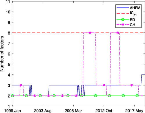
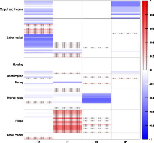
For most of the periods, our AHFM estimates three factors. This pattern is interrupted during the recent financial crisis, where it provides two factors, and after May 2018, where it estimates four factors. In order to economically identify the estimated factors, Figures A.3 and A.4 illustrate the factor loadings matrices estimated for January 1999 and June 2018, respectively.¹⁴ The additional sparsity in the non zero factor groups induced by the AFHM considerably simplifies factor allocation to economic sectors. In fact, for the period prior to June 2018, the latent factors can be interpreted as real activity, price, and interest rate factors.¹⁵ Starting from June 2018, we obtained one additional factor that represents variables in industrial production. These results are inline with the factor associations described by McCracken and Ng (2016) who employ a similar dataset as in our study.¹⁶ McCracken and Ng (2016) find a total eight factors as guided by the PC_p criteria developed in Bai and Ng (2002). However, they show that the fifth through eighth factors have noticeably less explanatory power compared to the first four factors and can be hardly assigned to specific economic groups. In contrast to these results, our AHFM directly discards the last four uninformative factors.

The number of factors estimated by the remaining methods are more diverse. The IC_p1 and IC_p2 select the maximum number of eight factors for all periods; however, as shown in the simulation study, those approaches tend to overestimate the number of factors, for a non trivial amount of correlation in the data. Moreover, the ED, ER, and GR methods estimate two factors. As indicated by the simulation results, these approaches provide a number of factors that are below the true quantity, for correlations in the idiosyncratic component and T > N, where N = 100, which approximately corresponds to the number of variables in our dataset. The CH approach by Caner and Han (2014) provides two factors for most of the periods, except for several occasions after the recent financial crisis, where it selects eight factors.

6.3. Results from the forecasting experiment

The results from our out-of-sample forecasting experiment are illustrated in Table 5. Generally, we can observe that it is cumbersome to outperform the benchmark AR model for long-term predictions (h = 6 or 12). However, for the one-step ahead forecasts, the factor-augmented AR processes offer considerably lower MSFEs compared to the benchmark model in most of the cases. Furthermore, the forecasting results highly depend on the number of factors included in the factor-augmented AR model. In fact, the MSFEs are lower if the number of factors is selected by the AHFM model for most of the time series and forecast horizons. More precisely, the AHFM shows considerable improvements in terms of predictability compared to the remaining selection methods for industrial production, the unemployment rate, manufacturing and trade industry sales, employees in manufacturing, and CPI. Moreover, if we consider the results across all variables in the dataset, which are illustrated in the last row of Table 5, we can see that the AHFM provides the best average predictive accuracy for all horizons. For h = 1 and h = 6 it offers a slight improvement compared to the benchmark AR model. Regarding the remaining methods, the IC_p1 and IC_p2 criteria provide the second-lowest MSFEs after the AHFM for total non agricultural employees and employees in manufacturing.

Table 5. Results from the forecasting experiment.

AHFM	ICp1	ICp2	ED	ER	GR	CH
IP	h = 1	0.82	0.92	0.92	0.96	0.96	0.96	0.91
	h = 6	0.97	1.01	1.01	1.00	1.00	1.00	1.00
	h = 12	1.00	1.00	1.00	1.02	1.02	1.02	1.01
UNRATE	h = 1	0.77	0.85	0.85	0.79	0.79	0.79	0.81
	h = 6	0.96	0.98	0.98	0.97	0.97	0.97	0.97
	h = 12	0.99	0.99	0.99	0.99	0.99	0.99	0.99
Mfg. & trade sales	h = 1	0.94	1.03	1.03	0.99	0.99	0.99	1.00
	h = 6	0.99	0.99	0.99	1.00	1.00	1.00	1.00
	h = 12	1.00	1.00	1.00	1.00	1.00	1.00	1.00
Empl. total nonag.	h = 1	0.97	0.90	0.90	1.00	1.00	1.00	0.97
	h = 6	1.02	1.08	1.08	1.04	1.04	1.04	1.04
	h = 12	1.04	1.05	1.05	1.04	1.04	1.04	1.05
Empl. mfg.	h = 1	0.77	0.81	0.81	0.88	0.88	0.88	0.87
	h = 6	0.84	0.86	0.86	0.90	0.90	0.90	0.90
	h = 12	0.95	0.96	0.96	0.97	0.97	0.97	0.97
CPI	h = 1	0.87	0.88	0.88	0.91	0.91	0.91	0.92
	h = 6	0.95	0.95	0.95	0.95	0.95	0.95	0.95
	h = 12	0.97	0.97	0.97	0.98	0.98	0.98	0.97
All variables	h = 1	0.96	0.98	0.98	0.99	0.99	0.99	0.98
	h = 6	0.98	1.11	1.11	0.99	0.99	0.99	1.02
	h = 12	1.00	1.76	1.76	1.00	1.00	1.00	1.16

Note: Our factor adaptive hierarchical factor model AHFM is compared to the methods by Bai and Ng (2002) IC_p1 and IC_p2, Onatski (2010) ED, Ahn and Horenstein (2013) ER and GR and Caner and Han (2014) CH, where the quantities represent the mean squared forecast errors relative to a univariate AR model.

7. Conclusions

We propose a hierarchical factor model for estimating the correct number of factors in approximate factor models. The model is based on a penalized maximum likelihood approach and incorporates an adaptive hierarchical lasso penalty function that allows for setting entire columns in the factor loadings matrix to zero, which corresponds to removing irrelevant factors. In our method, the estimated number of factors is the number of non zero columns in the estimated factor loadings matrix. Additionally, our method introduces sparsity in the non zero columns of the factor loadings matrix. Thus, it is able to simultaneously estimate pervasive and weak factors.

We prove average consistency under the Frobenius norm for the factor loadings of the relevant factors estimated based on our method. At the same time, the hierarchical factor model shrinks the factor loadings of the uninformative factors toward zero, with probability tending to one. Hence, our method is able to consistently estimate the correct number of factors.

In the simulation studies, we analyze the selection accuracy of our hierarchical factor model with respect to the chosen number of factors. The results reveal that our method selects the correct number of factors in finite samples in the majority of cases. In particular, our method performs very well for data with cross-sectional and serial correlation, showing typically fewer deviations from the correct number of factors compared to existing approaches. In this setting, we also note that the method of Bai and Ng (2002) tends to highly overestimate the correct number of factors. Furthermore, our method detects the true number of factors in almost all times, as both the time dimension T and cross-sectional dimension N increase.

In an empirical application, we focus on an out-of-sample forecasting experiment of time series in a large-dimensional macroeconomic dataset based on factor-augmented autoregressive processes. The results reveal lower mean squared forecast errors for an approximate factor model if the number of factor is selected by our method.

The focus of this article is on the static factor model representation. However, it would be interesting to analyze a possible extension of the hierarchical factor model to the dynamic factor model framework, by allowing for dynamics in the latent factors. This might be beneficial for the analysis of factor-augmented vector autoregressive models, as those require the selection of economically interpretable latent factors. Furthermore, it is crucial to include the correct number of common factors, to avoid any inconsistency in estimating the space spanned by the structural shocks. We leave this aspect for future research.

Acknowledgements

For helpful comments on an earlier draft of the article, we would like to thank Ralf Brüggemann, Mehmet Caner, participants of the 70th European Meeting of the Econometric Society, the 1st Vienna Workshop on Economic Forecasting, and the 6th RCEA Time Series Econometrics Workshop.

Notes

1. In the simulation studies and in the empirical application, we obtained identical results when considering group weights constructed on the basis of factor loadings estimated using unpenalized QML.

2. In general, it is also possible to post- and pre-multiply F₀ and ${\mathrm{\Lambda }}_0^{\prime }$ by an arbitrary non singular matrix P and its inverse P⁻¹, respectively.

3. As shown in Horn and Johnson (2012) only the rotation by a unitary generalized (signed) permutation matrix preserves the l₁-norm.

4. The pervasiveness assumption implies that the r largest eigenvalues of ${\mathrm{\Lambda }}_0^{\prime }{\mathrm{\Lambda }}_0$ diverge at the rate 𝒪(N).

5. For the N×r matrix Λ₀, we have that $\Vert {\mathrm{\Lambda }}_0\Vert \le \sqrt{Nr}{\Vert {\mathrm{\Lambda }}_0\Vert }_{\mathrm{\infty }}$, see e.g., Horn, and Johnson (2012). As Assumption 3.31 restricts the number of non zero elements in Λ₀ to be proportional to N^β, we have that $\Vert {\mathrm{\Lambda }}_0\Vert \le \sqrt{N^{\beta }}{\Vert {\mathrm{\Lambda }}_0\Vert }_{\mathrm{\infty }}$.

6. The restriction on the relation between N and T, p²log⁡N = o(T), is similar to the restrictions imposed in comparable research articles dealing with sparsity in approximate factor models. E.g., Bai and Liao (2016), who introduce an l₁-norm penalized maximum likelihood approach in the AFM for estimating a sparse idiosyncratic error covariance matrix, require the restriction log⁡N = o(T) for consistency. Moreover, Fan, Liao, and Mincheva (2013) impose the restriction $\log N=o(T^{\gamma /6})$, where γ is a positive constant, such that their POET estimator for the error covariance matrix is consistent.

7. While β > 0 is sufficient for the consistency of the individual loadings, the consistency of the individual factor estimates requires $\beta >1/3$, as shown by Bai and Ng (2023).

8. Lemma S.2.1 in the Supplement shows that optimizing either with the hierarchical penalty function or with the alternative penalty function (4.1(4.1) $$\begin{array}{l}\nu \sum _{k=1}^p{d}^{(k)}+\sum _{k=1}^p{\left(d^{(k)}\right)}^{-1}{\omega }^{(k)}\sum _{i=1}^N\left|{\lambda }_i^{(k)}\right|,\end{array}$$(4.1) ) yields equivalent solutions.

9. In all our simulation studies, we set J = 6.

10. All cardinalities are rounded to the smaller integer values.

11. Bai and Ng (2002) propose four additional estimators that incorporate a different specification of the information criteria compared to $I{C}_{p_1}$ and $I{C}_{p_2}$. As the selection results in the simulation studies provided by Bai and Ng (2002) for these estimators are similar to those of $I{C}_{p_1}$ and $I{C}_{p_2}$, we focus only on the latter two.

12. See Onatski (2010) for the implementation details of ξ.

13. Also in this case we set $k=1,\dots ,p$.

14. Since the factor loadings qualitatively do not change for the remaining subperiods for which the AHFM model estimates the same number of factors as at these two dates, we illustrate only the estimates for the first periods, where three and four factors are estimated.

15. The AHFM excludes the interest rate factor during periods when it provides solely two factors.

16. Our analysis uses an extended dataset that includes the time series data until December 2018, whereas McCracken and Ng (2016) analyze the data until December 2014.

Appendix

A Figures

Figure 2. Eigenvalue distribution for simulated data with 1 strong factor for T = 100, based on the first weak factor specification in the second simulation design.

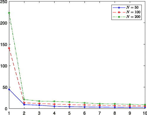
Figure 3. Eigenvalue distribution for simulated data with 1 strong and 3 weak factors for T = 100, based on the second weak factor specification in the second simulation design.

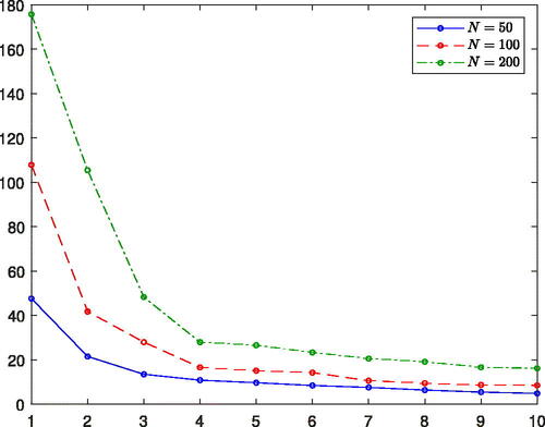
Figure 4. Factor loadings matrix for the adaptive HFM in January 1999. The factors are abbreviated as follows: ’RA’ real activity, ’P’ price, and ’IR’ interest rate.

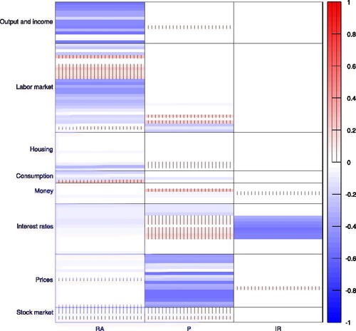
Figure 5. Factor loadings matrix for the adaptive HFM in period June 2018 The factors are abbreviated as follows: ’RA’ real activity, ’P’ price, ’IR’ interest rate, ’IP’ industrial production.

References

- Ahn, S. C., Horenstein, A. R. (2013). Eigenvalue ratio test for the number of factors. Econometrica 81(3):1203–1227.
- Bai, J., Li, K. (2012). Statistical analysis of factor models of high dimension. The Annals of Statistics 40(1):436–465.
- Bai, J., Li, K. (2016). Maximum likelihood estimation and inference for approximate factor models of high dimension. Review of Economics and Statistics 98(2):298–309.
- Bai, J., Liao, Y. (2016). Efficient estimation of approximate factor models via penalized maximum likelihood. Journal of Econometrics 191(1):1–18. 10.1016/j.jeconom.2015.10.003
- Bai, J., Ng, S. (2002). Determining the number of factors in approximate factor models. Econometrica 70(1):191–221. 10.1111/1468-0262.00273
- Bai, J., Ng, S. (2013). Principal components estimation and identification of static factors. Journal of Econometrics 176(1):18–29.
- Bai, J., Ng, S. (2023). Approximate factor models with weaker loadings. Journal of Econometrics235(2):1893–1916.
- Bai, J., Wang, P. (2014). Identification theory for high dimensional static and dynamic factor models. Journal of Econometrics 178(2):794–804. 10.1016/j.jeconom.2013.11.001
- Bernanke, B. S., Boivin, J., Eliasz, P. (2005). Measuring the effects of monetary policy: A factor-augmented vector autoregressive (FAVAR) approach*. Quarterly Journal of Economics 120(1):387–422. 10.1162/qjec.2005.120.1.387
- Bien, J., Tibshirani, R. J. (2011). Sparse estimation of a covariance matrix. Biometrika 98(4):807–820. 10.1093/biomet/asr054 23049130
- Boivin, J., Ng, S. (2006). Are more data always better for factor analysis?. Journal of Econometrics 132(1):169–194. 10.1016/j.jeconom.2005.01.027
- Caner, M., Han, X. (2014). Selecting the correct number of factors in approximate factor models: The large panel case with group bridge estimators. Journal of Business & Economic Statistics 32(3):359–374. 10.1080/07350015.2014.880349
- Chamberlain, G., Rothschild, M. (1983). Arbitrage, factor structure, and mean-variance analysis on large asset markets. Econometrica 51(5):1281. 10.2307/1912275
- Chan, J., Leon-Gonzalez, R., Strachan, R. W. (2018). Invariant inference and efficient computation in the static factor model. Journal of the American Statistical Association 113(522):819–828. 10.1080/01621459.2017.1287080
- Chudik, A., Pesaran, M. H., Tosetti, E. (2011). Weak and strong cross-section dependence and estimation of large panels. The Econometrics Journal 14(1):45–90.
- Daniele, M., Pohlmeier, W., Zagidullina, A. (2020). Sparse Approximate Factor Estimation for High-Dimensional Covariance Matrices, Working Paper series 20-03. Riverside, CA: Rimini Centre for Economic Analysis.
- Fan, J., Fan, Y., Lv, J. (2008). High dimensional covariance matrix estimation using a factor model. Journal of Econometrics 147(1):186–197. 10.1016/j.jeconom.2008.09.017
- Fan, J., Liao, Y., Mincheva, M. (2013). Large covariance estimation by thresholding principal orthogonal complements. Journal of the Royal Statistical Society Series B: Statistical Methodology 75(4):603–680. 10.1111/rssb.12016
- Forni, M., Reichlin, L. (1998). Let’s get real: A factor analytical approach to disaggregated business cycle dynamics. Review of Economic Studies 65(3):453–473. 10.1111/1467-937X.00053
- Freyaldenhoven, S. (2022). Factor models with local factors—determining the number of relevant factors. Journal of Econometrics 229(1):80–102. 10.1016/j.jeconom.2021.04.006
- Freyaldenhoven, S. Freyaldenhoven, S. (2023). Identification Through Sparsity in Factor Models: The l1-Rotation Criterion, Working Paper 20-25. Philadelphia, PA: Federal Reserve Bank of Philadelphia.
- Giannone, D., Reichlin, L., Sala, L. (2002). Tracking greenspan: Systematic and unsystematic monetary policy revisited. CEPR discussion papers 3550. C.E.P.R. Discussion Papers.
- Hallin, M., Liška, R. (2011). Dynamic factors in the presence of blocks. Journal of Econometrics 163(1):29–41. 10.1016/j.jeconom.2010.11.004
- Horn, R. A., Johnson, C. R. (2012). Matrix Analysis. Cambridge, UK: Cambridge University Press.
- Jennrich, R. I. (2006). Rotation to simple loadings using component loss functions: The oblique case. Psychometrika 71(1):173–191. 10.1007/s11336-003-1136-B
- Kaufmann, S., Schumacher, C. (2019). Bayesian estimation of sparse dynamic factor models with order-independent and ex-post mode identification. Journal of Econometrics 210(1):116–134. 10.1016/j.jeconom.2018.11.008
- Lawley, D., A., Maxwell, (1971). Factor Analysis as a Statistical Method, 2nd ed. London: Butterworths.
- Liu, X., Wallin, G., Chen, Y., Moustaki, I. (2023). Rotation to sparse loadings using [formula: see text] losses and related inference problems. Psychometrika 88(2):527–553. 10.1007/s11336-023-09911-y 37002429
- McCracken, M. W., Ng, S. (2016). FRED-MD: A monthly database for macroeconomic research. Journal of Business & Economic Statistics 34(4):574–589. 10.1080/07350015.2015.1086655
- Nesterov, Y. (1983). A method for solving the convex programming problem with convergence rate O(1/k2). Soviet Mathematics - Doklady 269:543–547.
- Onatski, A. (2010). Determining the number of factors from empirical distribution of eigenvalues. Review of Economics and Statistics 92(4):1004–1016. 10.1162/REST_a_00043
- Onatski, A. (2012). Asymptotics of the principal components estimator of large factor models with weakly influential factors. Journal of Econometrics 168(2):244–258.
- Ross, S. A. (1976). The arbitrage theory of capital asset pricing. Journal of Economic Theory 13(3):341–360. doi:10.1016/0022-0531(76)90046-6
- Stock, J. H., Watson, M. W. (2002). Macroeconomic forecasting using diffusion indexes. Journal of Business & Economic Statistics 20(2):147–162. doi:10.1198/073500102317351921
- Stock, J. H., Watson, M. W. (2005). Implications of Dynamic Factor Models for VAR Analysis, NBER Working Paper w11467.
- (2016). Dynamic factor models, factor-augmented vector autoregressions, and structural vector autoregressions in macroeconomics. In: Handbook of Macroeconomics, Vol. 2. Amsterdam, Netherlands: Elsevier, pp. 415–525.
- Trzcinka, C. (1986). On the number of factors in the arbitrage pricing model. The Journal of Finance 41(2):347–368. doi:10.1111/j.1540-6261.1986.tb05041.x
- Uematsu, Y., Yamagata, T. (2022). Estimation of sparsity-induced weak factor models. Journal of Business & Economic Statistics41(1):213–227.
- Yuan, M., Lin, YI. (2006). Model selection and estimation in regression with grouped variables. Journal of the Royal Statistical Society Series B: Statistical Methodology 68(1):49–67. doi:10.1111/j.1467-9868.2005.00532.x
- Zhao, W., Zhang, R., Liu, J. (2014). Sparse group variable selection based on quantile hierarchical lasso. Journal of Applied Statistics 41(8):1658–1677. doi:10.1080/02664763.2014.888541
- Zhou, N., Zhu, JI. (2010). Group variable selection via a hierarchical lasso and its oracle property. Statistics and Its Interface 3(4):557–574. doi:10.4310/SII.2010.v3.n4.a13
- Zou, H. (2006). The adaptive lasso and its oracle properties. Journal of the American Statistical Association 101(476):1418–1429. doi:10.1198/016214506000000735