Up-and-Down Designs for Selecting the Dose with Maximum Success Probability

Abstract

Assume that the probability of success is unimodal as a function of dose, such as may be the case when too much of a drug is toxic and too little is ineffective. We characterize a class of up-and-down designs, that is, treatment allocation methodologies, for identifying the dose that maximizes the patients' success probability. These designs are constructed to use accruing information to limit the number of patients that are exposed to doses with high probabilities of failure. This treatment allocation procedure is motivated by Kiefer–Wolfowitz's stochastic approximation procedure. However, we take the response to be binary and the possible treatment space to be a lattice. The procedure is shown to allocate treatments to pairs of subjects in a way that causes the treatment distribution to center around the treatment with maximum success probability. The procedure defines a nonhomogeneous random walk, so well-known theory is used to explicitly characterize the treatment distribution. As an estimator of the best dose, the mode of the empirical treatment distribution is shown to converge faster than does the last dose allocated, which is used as an estimator of the optimal dose in stochastic approximation procedures.

Keywords:

• Constant gain stochastic algorithm
• Dose-finding
• Efficacy
• Markov chains
• Optimal dose
• Phase I/II clinical trial
• Random walk designs
• Stationary treatment distribution
• Stochastic approximation
• Toxicity
• Unimodality

Subject Classifications:

• 60J10
• 60J20
• 62K99
• 62L05

1. INTRODUCTION

Up-and-down rules are procedures that specify the treatment for the next trial to be one level higher, one level lower, or the same as the treatment selected for the current trial. Von Bekesy (1947) and Dixon and Mood (1948) analyzed a version for estimating the 50th percentile of an increasing response function. Derman (1957) extended the procedure for estimating any quantile. Wetherwill (1963), Dixon (1965), Tsutakawa (1967), and many others studied modifications of Dixon and Mood's up-and-down design. Until Durham and Flournoy (1994), aside from Derman (1957), up-and-down procedures were studied by simulation and/or by making parametric assumptions concerning the success probability function.

Durham and Flournoy (1994 1995) and Flournoy, Durham, and Rosenberger, (1995) introduced several Markovian up-and-down procedures for estimating an arbitrary quantile for any increasing response function. Giovagnoli and Pincacuda (1998) generalized these procedures and determined that, within a broad class of Markovian up-and-down procedures, Durham and Flournoy's original Durham and Flournoy 1994 procedure was optimal in the sense that the resulting treatment distribution was most peaked around the target quantile. Many other dose-finding procedures have since been studied assuming increasing response functions.

This procedure differs significantly from other up-and-down designs in the literature in that it is to be used when the probability of response is a unimodal function, rather than an increasing one. We consider a response to be a success or failure and we call the dose having maximum probability of success the optimal dose. Because the proposed designs cluster treatments around the optimal dose given a unimodal response function, they are called optimizing up-and-down designs. The main results in this papers were announced by Kpamegan and Flournoy in Kpamegan and Flournoy 2001. This paper provides the theoretical basis for the results and additional examples.

Li, Durham, and Flournoy (1995) give conditions for the success probability function to be unimodal when it is constructed by combining a toxicity model and an efficacy model according to contingent response model. Although these conditions have been found to hold in many situations, in general, the probability of success need not be a unimodal function of dose. This is exemplified in Murtaugh and Fisher (1990) and Heise and Meyers (1996). The conditions for unimodality cannot be verified by a researcher a priori, and further research is required to establish practical guidelines for making the unimodality assumption. Some other sequential design approaches for unimodal response functions are given by Li, Durham, and Flournoy (1995), Thall and Russell (1998), O'Quigley, Hughes, and Fenton (2001), Braun (2002), and Hardwick, Meyer, and Stout (2003).

In Section 2, we provide a technical motivation for the proposed procedure. In Section 3, we define the optimizing up-and-down designs under consideration. In Section 4, we give the treatment transition probabilities. In Section 5, we derive the stationary treatment distribution. In Section 6, we show that the stationary treatment distribution is unimodal, and in Section 7 we show the empirical treatment mode converges to a near neighborhood of the optimal dose. Finally, we compare the performance of the up-and-down with stochastic approximation in Section 8.

2. TECHNICAL MOTIVATION: STOCHASTIC APPROXIMATION

Kiefer and Wolfowitz (1952) defined the following procedure for sequential estimation of the maximum of a regression function that has a maximum at the unknown point μ. This procedure has been widely researched; see, for example, Chung (1954), Derman (1956), Sacks (1958), and Pflug (1996). Our motivation is its application to binary responses in the context studied by Durham, Flournoy, and Li (1998). The regression function is α(x) = P(success|x) and  = 1 − α(x). Let μ denote the optimal dose. Suppose that α(x) is strictly increasing for x < μ and strictly decreasing for x > μ. Define infinite sequences of positive numbers {a _n } and {c _n } such that .

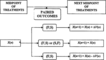
Subjects are treated in pairs at dose levels determined recursively by a _n and c _n . Let X(n) be the midpoint of the dose interval for the nth pair. If the nth pair of subjects has been treated at X(n) − c _n and X(n) + c _n , the midpoint of the (n + 1)th pair is

where Y ₁(n) and Y ₂(n) are Bernoulli random variables with success probabilities α(X(n) + c _n ) and α(X(n) − c _n ), respectively. Conditional on X(n), Y ₁(n) and Y ₂(n) are independent. The stochastic approximation estimator of the dose with maximum probability of response is defined recursively by  = X(n).

The scheme we propose is similar to stochastic approximation, but the treatment space is restricted to a discrete lattice and changes in treatment levels from trial to trial are limited to adjacent doses.

3. AN OPTIMIZING UP-AND-DOWN DESIGN

Let subjects be treated in pairs, and let X(n) denote the midpoint of the dose interval for the nth pair of subjects, where the possible midpoints come from a finite set: Ω = {x ₁,…, x _K }. We refer to {X ₁(n)} and {X ₂(n)}, respectively, as the left sequence and right sequence of treatment pairs. For notational convenience, we assume that the interval between possible dosage midpoints is a positive constant Δ and that the interval between pairs of treatments is the same constant Δ. Thus {X ₁(n)} and {X ₂(n)} assume values on the lattice of points and , respectively. Now the optimizing up-and-down design for selecting the dose with maximum success probability is defined by the following algorithm, with adjustments at the boundaries of the treatment space:

If the nth pair of subjects has been treated at and , the midpoint of the (n + 1)th pair is

where

On the boundaries, when the dose would otherwise go down or up, it stays constant. Figure 1 gives a graphical presentation of the procedure on the interior of the treatment space. The notation (F, S) indicates that treatment at resulted in a failure while treatment at resulted in success. Analogously, we define (S, F), (S, S), and (F, F). For each pair of subjects, we refer to the one treated at the lower (higher) dose as subject 1 (2) of the nth pair. Note from equation (3.1) that if X(n) = x _k , then, except on the boundary of the treatment space, the possible treatment levels for the individuals in the (n + 1)th pair are

while the sequence of treatments generated in stochastic approximation converges to a point, the sequence generated by the up-and-down procedure converges to a stationary distribution. This stationary distribution is described in terms of the transition probabilities between treatments.

Figure 1 Optimizing up-and-down design. The notation (F, S) indicates that treatment at resulted in a failure while treatment at resulted in success. (S, F), (S, S), and (F, F) are analogously defined.

4. TRANSITIONS BETWEEN TREATMENTS

Let p _k , q _k , and r _k denote, respectively, the probability that the treatment dosage for the left subject will move down from level to , up from level to , and stay at level , with p _k  + q _k  + r _k  = 1. Assume that subject 1 of the nth pair has just been allocated treatment . Then for the left sequence on the interior of the treatment space, the treatment transition probabilities for k = 2,…, K − 1 are

At the boundaries p ₁ = q _K  = 0, so that and . The resulting one-step transition probability matrix is

5. THE STATIONARY TREATMENT DISTRIBUTION

The right sequence has an identically shaped stationary treatment distribution that is shifted Δ to the right of the one for the left sequence. As long as p _k  > 0 (k = 2,…, K), q _k  > 0 (k = 1,…, K − 1), and r _k  > 0 for some k = 1,…, K, the allocation of treatments for each sequence describes an irreducible recurrent Markov chain, and thus the left and right stationary distributions exist (cf. Harris, 1952). Let π = (π₁,…, π _K ) and π′ = (π₁′,…, π _K ′) denote the left and right stationary distribution, respectively, where and . The stationary treatment distributions π and π′ are defined, respectively, on Ω _L and Ω _R . Theorem 5.1 gives the stationary treatment distribution for the subjects in the left sequence. Results for the right sequence are obtained analogously.

Theorem 5.1

The stationary treatment probabilities for the left sequence of subjects are

where

Proof

The stationary treatment distribution for each sequence is obtained by solving the balance equations: π _k  = π _k−1 q _k−1 + π _k r _k  + π _k+1 p _k+1, k = 1,…, k, yielding

where

(cf. Karlin and Taylor, 1975). Inserting (4.1) into (5.2) yields

But for k = 2,…, K, because . Hence λ _k reduces to

Inserting (5.3) into (5.1) and solving for yields the result.

Corollary 5.1

The right sequence has an identically shaped stationary treatment distribution that is shifted Δ to the right of the one for the left sequence.

Corollary 5.2

Assume subjects are randomly assigned within each pair to the left and right sequences. Then the combined stationary treatment distribution is a mixture of the left and right treatment distributions with mixing parameter 1/2 and support on the combined treatment space

Proof

P{subject is treated at dose {subject is treated at dose x|left sequence} + {subject is treated at dose x|right sequence}.

Note that Ω _L and Ω _R each has K treatments levels, whereas Ω _C has K + 1 treatments levels.

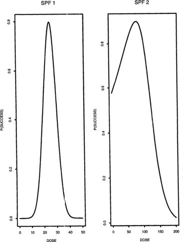
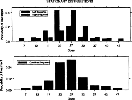
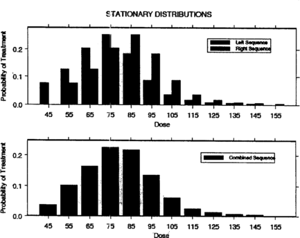
Examples of success probability functions (SPFs) that we will use later in this paper are given in Figure 2. For SPF 1, the success probability function is symmetric around its maximum at μ = 25. It is close to zero for doses less than 10 and greater than 40. SPF 2 is right skewed with maximum success probability at μ = 80. Figure 3 shows the stationary treatment distributions generated by the left and right sequences, respectively, using SPF 1; finally, the resulting combined stationary treatment distribution is displayed at the bottom of the figure. Figure 4 is obtained similarly using SPF 2.

Figure 2 SPFs 1 and 2; their optimal doses are μ = 25 and μ = 80, respectively.

Figure 3 Stationary treatment distributions under SPF 1.

Figure 4 Stationary treatment distributions under SPF 2.

6. UNIMODALITY OF THE STATIONARY TREATMENT DISTRIBUTION

We define a modal set and unimodality on a lattice before establishing the unimodality of the stationary treatment distribution in Theorem 6.1.

Definition 6.1

The set M(π) of points of absolute maximum for π is called the modal set. The minimum point of M(π) will be called the mode of π.

Definition 6.2 (Keilson and Gerber, 1971)

A distribution π = {π _k } with all support on the lattice of integers is said to be unimodal if there exists at least one integer M such that

Note if π is unimodal, then for all m ∊ M(π), x < m ≤ y implies π(x) ≤ π (m) ≥ π(y).

Definition 6.3

Let 𝕜 be the largest integer such that

Theorem 6.1

If α(x) is unimodal with mode μ, the stationary treatment distributions of the left sequence and right sequence are unimodal with mode  = x _𝕜 − Δ/2 and  = x _𝕜 + Δ/2, respectively. Furthermore, if λ_𝕜 + 1 = 1, the modal set contains more than one dose.

Proof

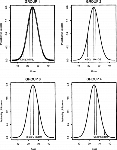
We give the proof for the left sequence. The proof for the right sequence is obtained analogously. Note from (5.2) that λ _k is the probability that the left sequence increases from divided by the probability it decreases from , and from (5.3), it is clear that λ _k only depends on the success probability function at and at . Consider the sequence of dose pairs divided into four groups (see Figure 5).

	Group 1 consists of the sequence below μ with the lower dose having a lesser success probability. For the values in this set, implies that , which implies that .
	Group 2 consists of the set of pairs that straddle μ with the success probability of the lower dose smaller than that of the higher dose. That is, and with , which implies that λ k  > 1. Note from (5.1) that π k  = π k−1λ k . Thus, π k  > π k−1 when λ k is produced by pairs in Group 1 or 2 because λ k  > 1. Hence π k increases over this region.
	Group 3 consists of the sets of pairs that straddle μ with the higher dose having a success probability not exceeding that of the smaller dose. That is, and with , which implies that . By Definition 6.1, the largest k in this set is 𝕜, so π k  < π𝕜, k < 𝕜. When λ k is produced by treatment pairs in Group 3, π k  ≤ π k−1 because λ k  ≤ 1. So over this set, π k is decreasing, but not necessarily strictly so. For the smallest k in Group 3, it follows that π k  ≤ π𝕜, and if equality is achieved the modal set contains more than one value.
	Group 4 consists of the set of pairs that are greater than μ, the smaller dose having a greater success probability. That is, with , which implies that . When λ k is produced by treatment pairs in Group 4, λ k  < 1 and hence π k  ≤ π k−1.

Hence π_𝕜 = max _k {π _k }, and x _𝕜 − Δ/2 is the mode of the left treatment sequence.

Figure 5 SPF 1 is marked with solid horizontal lines at pairs of doses selected from four groups used in the proof of Theorem 6.1. The optimal dose μ = 25 is also marked with a solid horizontal line. Group 1 consists of treatment pairs below μ. Group 2 consists of pairs that straddle μ with the success probability of the lower dose smaller than that of the higher dose. Group 3 consists of pairs that straddle μ with the higher dose having a success probability not exceeding that of the smaller dose. Group 4 consists of pairs that are greater than μ with the smaller dose having a greater success probability.

Theorem 6.2

The combined stationary treatment distribution is unimodal with the mode at if π_𝕜 − 1 > π_𝕜 + 1 and if π_𝕜 − 1 < π_𝕜 + 1; the modal set contains {,} if π_𝕜 − 1 = π_𝕜 + 1.

Proof

Recall that the right sequence has an identically shaped stationary distribution that is shifted Δ to the right of the one for the left sequence. So over the combined treatment space,

the stationary treatment probabilities are

Now, because π_𝕜 ≥ π_𝕜 − 1 ≥···≥ π₁ and π_𝕜 ≥ π_𝕜 + 1 ≥···≥ π _K , it follows that

If π_𝕜 − 1 > π_𝕜 + 1, then , and the combined stationary treatment distribution is unimodal with the mode at  = x _𝕜 − Δ/2. Similarly, if π_𝕜 − 1 < π_𝕜 + 1, then , and the combined stationary treatment distribution is unimodal with the mode at  = x _𝕜 + Δ/2. Finally, if π_𝕜 − 1 = π_𝕜 + 1, then , and the combined stationary treatment distribution is unimodal with the modal set including  = x _𝕜 − Δ/2 and  = x _𝕜 + Δ/2.

Tables 1 and 2 show how Theorem 6.2 applies to the success probability-functions shown in Figure 2. In particular, Tables 1 and 2 give the mode x _𝕜 − Δ/2 of the stationary treatment distribution of the left sequence for five different values of Δ along with λ_𝕜 − 1, λ_𝕜, and λ_𝕜 + 1 as well as the possible treatment values. Note from the tables that if the mode μ of the success probability function is among possible treatments, then x _𝕜 − Δ/2 is equal to μ. Otherwise, x _𝕜 is close to μ. We make this notion of closeness more precise in the next section.

Table 1. Stationary treatment distribution characteristics for the left sequence under SPF 1 in which μ = 25

Δ		λ𝕜 − 1	λ𝕜	λ𝕜 + 1	Possible treatment values
1	24, 25	1.531	1.304	1	{9, 10,…,24,…,44}
2	24	2.368	1.531	.653	{4, 6,…,24,…,39, 42}
3	24	3.215	1.597	.423	{9, 12,…,24,…,42}
4	24	3.864	1.547	.311	{0, 4,…,24,…,42}
5	20, 25	1.921	4.413	1	{0, 5,…,20,…,40}

Table 2. Stationary treatment distribution characteristics for the left sequence SPF 2 in which μ = 80

Δ		λ𝕜 − 1	λ𝕜	λ𝕜 + 1	Possible treatment values
3	78	1.083	1.037	.983	{3,…,78,…,177}
5	75	1.236	1.337	.999	{10, 15,…,75,…, 180}
8	76	1.428	1.162	.820	{4, 12,…,76,…,188}
10	75	1.609	1.235	.740	{5, 15,…,75,…,195}
15	75	2.047	1.252	.471	{15,…,75,…,195}

7. CONVERGENCE OF THE EMPIRICAL TREATMENT MODE

Theorem 7.1 shows that the mode of the asymptotic treatment distribution can be bounded near the dose with maximum success probability, and this bound is tighter if the success probability function is symmetric.

Theorem 7.1

Let α(x) be the unimodal success probability function. Then  − Δ ≤ μ < . Furthermore, if α(x) is symmetric about its mode μ, then μ is within Δ/2 of the asymptotic treatment x _𝕜, that is, or equivalently  ≤ μ ≤ .

Proof

Recall from the proof of Theorem 6.2 that is the most frequent treatment pair in Group 2. Therefore,

Now consider α(x) to be symmetric about μ. If in addition to α(x) being symmetric about , then we would have . The dose pairs in Group 2 have see Figure 5. Therefore, these paired doses are not equidistant from μ. Indeed, because the dose pairs are in Group 2. Furthermore, note that because , it follows that . This inequality simplifies to . Now note that because the dose pair is in Group 2, they straddle μ and hence, . Together, these two relations give the result.

Definition 7.1

Let the mode of the stationary treatment distribution for the combined sequence and define  = ( + )/2.

Corollary 7.1

For any SPF, (1) 0 < |μ − |<Δ if  = , (2) 0 < |μ − |<2Δ if  = , and (3) .

Proof

From Theorem 6.2, the mode of the stationary treatment distribution of the combined sequence is and/or and from Theorem 7.1,  − Δ < μ < . So if  = , then  =  + Δ. Hence  − Δ < μ <  + Δ, that is, 0 < |μ − |<Δ. If  = , then  =  − Δ. Therefore ( − Δ) − Δ < μ <  or 0 < |μ − |<2 Δ. Finally, because  = ( + )/2, using,  =  + Δ, we can write . Therefore, .

Corollary 7.2

For a symmetrical SPF, (1) 0 < |μ − |<Δ if  = , (2) 0 < |μ − |<Δ if  = , and (3) .

Proof

Follows from the proof of Corollary 7.1 with  ≤ μ ≤ .

8. COMPARISON WITH STOCHASTIC APPROXIMATION

For estimating μ, we compare the mean squared error (MSE) of  = ( + )/2 from the optimizing up-and-down design with X(n) from stochastic approximation. For stochastic approximation, we use a _n  − a/n and c _n  = c/n ^1/4, where a and c are positive constants. These sequences provide optimal convergence rates (cf. Wasan, 1969). Also, we start the stochastic approximation procedure with a ₁/c ₁ = Δ. For this comparison, we used SPFs 1 and 2 as shown in Figure 2. Recall that for SPF 1, the optimal dose is μ = 25, and the probability of success is close to zero for doses less than 10 and greater than 40. Recall also that SPF 1 is symmetric about μ. SPF 2 is right skewed and its maximum is at μ = 80.

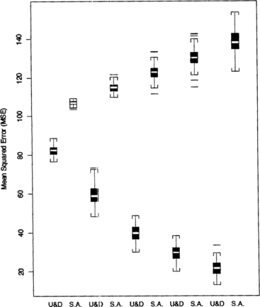
Each MSE, E( − μ)² for the optimizing up-and-down design and E(X(n) − μ)² for stochastic approximation, was simulated using 2,000 estimates of the optimal dose under a variety of conditions. The simulated distribution of the MSEs are summarized in side-by-side boxplots in Figures 6-8 for comparison. The results suggest that the up-and-down procedure produces estimates with smaller MSE than does stochastic approximation.

Figure 6 Comparison of MSEs for sample sizes n = 10, 20, 30, 50, and 100 under SPF 1. The starting midpoint is fixed at X(1) = 15 and the step size is fixed at Δ = 3.

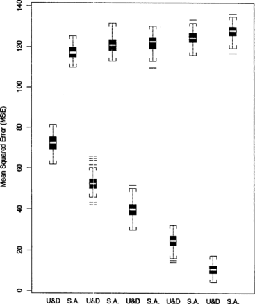
Figure 7 Comparison of MSEs for step sizes Δ = 1, 2, 3, 4, and 5 under SPF 1. The starting midpoint is fixed at X(1) = 15 and sample size is fixed at n = 30.

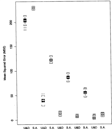
Figure 8 Comparison of MSEs for starting midpoints X(1) = 10, 15, 17.5, 20, and 25 under SPF 1. The step size is fixed at Δ = 3 and the sample size is fixed at n = 30.

8.1. Sample Size Effect

Figure 6 displays boxplots of the MSEs for sample sizes ranging from 10 to 100. They are computed with the step size fixed at Δ = 3 and the initial midpoint of dose pairs fixed at X(n) = 15, and they clearly show that the up-and-down procedure performs better than stochastic approximation for all sample sizes. The larger the sample size, the better it is.

8.2. Step Size Effect

Side-by-side boxplots for each step size 1, 2, 3, 4, and 5, in Figure 7 again show that the optimizing up-and-down design performs better than stochastic approximation. They are computed starting both designs at the lowest possible dose midpoint. X(1) = 15, with sample size n = 30. Simulations have also shown that when the step size is very small and the first treatments are at the lowest possible pair of doses, neither procedure moves out of the tail of the success probability function and the two procedures generate estimates with similar MSEs. Therefore, if one observes a series of trials without success, some intervention should be taken. For example, Δ could be increased, or a jump could be taken with probability going to zero as n increases.

8.3. Starting Point Effect

Figure 8 displays side-by-side boxplots of the MSEs for starting treatment midpoints ranging from X(1) = 10 in the extreme lower tail of the success probability function to X(1) = 25, the optimal dose. The MSEs are large for X(1) = 10, where the curve is very low and almost flat. This demonstrates again that if initial observations are made near the tails of a bell-shaped curve, convergence to the mode will be very slow. The reason is that in the tail of the response function the difference between the responses will be close to zero almost always. When starting treatment midpoints are close to the mode, the MSEs are small and similar for the two procedures. In general, however, the up-and-down procedure generates estimates with smaller MSEs.

9. CONCLUDING COMMENTS

We have presented an optimizing up-and-down design that causes the distribution of treatments to cluster around the dose with maximum success probability. A theoretical analysis of the asymptotic behavior of this design was given. A brief analysis of the small sample behavior of the treatment mode, as an estimator of the optimal dose, was based on simulation. Note, however, that because the design produces a nonhomogenous random walk, exact moments can be calculated for the number of treatments and successes at each dose, as was done for biased coin up-and-down designs by Durham et al. (1995) and Flournoy, Durham, and Rosenberger, (1995).

Hardwick and Stout (1998) suggest a way to improve convergence of the empirical mode estimator, which will also help move quickly away from doses with low probability of success. They suggest that when the response to treatment for both subjects in a pair is either success or failure, the next dose be increased or decreased according to the flip of an unbiased coin. We call this procedure the optimizing up-and-down design with randomized ties. We derived an expression for the stationary treatment distribution assuming randomized ties and found, not surprisingly, that it also clusters treatments around the optimal dose. Evaluating it assuming SPF 1 and SPF 2, we found that the procedure with randomized ties does converge faster, but it converges to a stationary treatment distribution that is more dispersive than without randomized ties. Thus there is a trade-off. One might consider using randomized ties initially, say, for the five pairs of subjects, as this would help the treatments move out of the tail of the success probability function, and then switch to nonrandomized ties.

If one can distinguish between failure types such as for toxic failures that occur if the dose is too high and the disease persistence if the dose is too low, one may decide to star; the experiment at a very low dose. In this case, we recommend beginning with the following dose escalation scheme: increase the dose until the first success (no toxicity and no disease failure) is observed and then begin the optimizing up-and-down design. It is also desirable to take failure type into account in the basic up-and-down procedure. This is not so easy to do. An attractive idea proposed by Flournoy (1985) was to increase the dose if a toxic response was observed and decrease the dose if disease persisted. This idea was studied via simulations by Gooley et al. (1994). The stationary treatment distribution resulting from this procedure centers treatments around the dose at which the “hazard” of the two failures are equal (see Li, Durham, and Flournoy, 1995, for elaboration). Ivanova (2003) rediscovers this fact and studies the distance between the mode of the treatment distribution and the point of maximum success.

Thus a challenge is to find a modification of the basic design that takes failure type into account and yet still clusters treatments around the dose with maximum success probability. Yet convergence of the estimator is so fast, outperforming stochastic approximation, that the optimizing up-and-down design should be considered (via simulation for particular expected scenarios) for human experiments. For animal experiments, the benefits of this design over current Phase I/II strategies are clear: fast convergence of the estimator will yield the best dose with few animals. Larger group sizes can be accommodated easily.

Notes

Recommended by D.S. Coad

REFERENCES

- Braun , T. ( 2002 ). The Bivariate Continual Reassessment Method: Extending the CRM to Phase I Trials of Two Competing Outcomes , Controlled Clinical Trials 23 : 240 – 256 .
- Chung , K. L. ( 1954 ). On a Stochastic Approximation Method , Annals of Mathematical Statistics 25 : 463 – 483 .
- Derman , C. ( 1956 ). Stochastic Approximation , Annals of Mathematical Statistics 27 : 879 – 886 .
- Derman , C. ( 1957 ). Non-parametric Up and Down Experimentation , Annals of Mathematical Statistics 28 : 795 – 799 .
- Dixon , W. J. ( 1965 ). Up-and-Down Method for Small Samples , Journal of the American Statistical Association 60 : 967 – 978 .
- Dixon , W. J. and Mood , A. M. (1948). A Method of Obtaining and Analyzing Sensitivity Data, Journal of American Statistical Association 43: 109–126.
- Durham , S. D. and Flournoy N. ( 1994 ). Random Walks for Quantile Estimation , in Statistical Decision Theory and Related Topics V , J. Berger and S. Gupta , eds., pp. 467 – 476 , New York : Spring-Verlag .
- Durham , S. D. and Flournoy , N. ( 1995 ). Up-and-Down Designs I: Stationary Treatmeat Distributions , in Adaptive Designs , IMS Lecture Notes—Monograph Series 25 , N. Flournoy and W. F. Rosenberger , eds., pp. 139 – 157 , Hayward : Institute of Mathematical Statistics .
- Durham , S. D. , Flournoy , N. , and Montazer-Haghighi , A. ( 1995 ). Up and-Down Designs II: Exact Treatment Moments , in Adaptive Designs , IMS Lecture Notes—Monograph Series 25 , N. Flournoy and W. F. Rosenberger , eds., pp. 158 – 178 , Hayward : Institute of Mathematical Statistics .
- Durham , S. D. , Flournoy , N. , and Li , W. ( 1998 ). A Sequential Design for Maximizing the Probability of a Favorable Response , Canadian Journal of Statistics 26 : 479 – 495 .
- Flournoy , N. ( 1985 ). Proposal made to the Seattle Bone Marrow Transplant Team during the preparation of the Adult Leukemia Center grant renewal .
- Flournoy , N. , Durham , S. D. , and Rosenberger , W. F. ( 1995 ). Toxicity in Sequential Dose-Response Experiments , Sequential Analysis 14 : 217 – 228 .
- Giovagnoli , A. and Pincacuda , N. ( 1998 ). Properties of Frequency Distributions Induced by General “Up-and-Down” Methods for Estimating Quantiles , Journal of Statistical Planning and Inference 74 : 51 – 63 .
- Gooley , T. A. , Martin , P. J. , Lloyd , D. F. , and Pettinger , M. ( 1994 ). Simulation as a Design Tool for Phase I/II Clinical Trials: An Example from Bone Marrow Transplantation , Controlled Clinical Trials 15 : 450 – 460 .
- Hardwick , J. P. and Stout , Q. ( 1998 ). Personal communication .
- Hardwick , J. , Meyer , M. C. , and Stout , Q. F. ( 2003 ). Directed Walk Designs for Dose Response Problems with Competing Failure Modes , Biometrics 59 : 229 – 236 .
- Harris , T. ( 1952 ). First Passage and Recurrence Distributions , Transactions of the American Mathematical Society 73 : 471 – 486 .
- Heise , P. A. and Meyers , R. H. ( 1996 ). Optimal Designs for Bivariate Logistic Regression , Biometrics 52 : 613 – 624 .
- Ivanova , A. ( 2003 ). A New Dose-Finding Design for Bivariate Outcomes , Biometrics 59 : 1001 – 1007 .
- Karlin , S. and Taylor , H. M. ( 1975 ). A First Course in Stochastic Processes , New York : Academic Press .
- Keilson , J. and Gerber . H. ( 1971 ). Some Results for Discrete Unimodality , Journal of American Statistical Association 66 : 386 – 389 .
- Kiefer , J. and Wolfowitz , J. ( 1952 ). Stochastic Approximation of the Maximum of a Regression Function , Annals of Mathematical Statistics 25 : 529 – 532 .
- Kpamegan , E. E. and Flournoy , N. ( 2001 ). An Optimizing Up and Down Design , in Optimum Design 2000 , A. C. Atkinson and B. Bogacka , eds., pp. 211 – 224 , the Netherlands : Kluwer Academic Publishers .
- Li , Z. , Durham , S. D. , and Flournoy , N. ( 1995 ). An Adaptive Design for Maximization of a Contingent Binary Response , in Adaptive Designs , IMS Lecture-Notes—Monograph Series 25 , N. Flournoy and W. F. Rosenberger , eds., pp. 179 – 196 , Hayward : Institute of Mathematical Statistics .
- Murtaugh , P. A. and Fisher , L. D. ( 1990 ). Bivariate Models of Efficacy and Toxicity in Dose-Ranging Trials , Communications in Statistics A—Theory & Methods 19 : 613 – 624 .
- O'Quigley , J. , Hughes , M. , and Fenton , T. ( 2001 ). Dose Finding Designs for HIV Studies , Biometrics 57 : 1018 – 1029 .
- Pflug , G. C. ( 1996 ). Optimization of Stochastic Models (The Interface between Simulation and Optimization) , New York : Kluwer Academic Publisher .
- Sacks , J. (1958). Asymptotic Distribution of Stochastic Approximation Procedures, Annals of Mathematical Statistics 29: 373–405.
- Thall , P. and Russell , K. ( 1998 ). A Strategy for Dose-Finding and Safety Monitoring Based on Efficacy and Adverse Outcomes in Phase I/II Clinical Trials , Biometrics 54 : 251 – 264 .
- Tsutakawa , R. K. ( 1967 ). Random Walk Design in Bio-Assay , Journal of American Statistical Association 62 : 842 – 856 .
- Von Bekesy , G. ( 1947 ). A New Audiometer , Acta Otolaryngology 35 : 411 – 422 .
- Wasan , M. T. ( 1969 ). Stochastic Approximation , Cambridge : University Press .
- Wetherwill , G. B. ( 1963 ). Sequential Estimation of Quantal Response Curves , Journal of Royal Statistical Society, Series B 25 : 1 – 48 .