Weighted Logrank Statistics in Sequential Tests

Abstract

Fully sequential generalization of some group sequential tests currently in use in clinical trials are considered. The model is censored data with random staggered entry, and it is used for the comparison of two treatments. Results show that the sequential tests can outperform group sequential tests and provide more information about the nature of relationship of the two treatments. Furthermore, they allow complete freedom in scheduling data evaluation.

Keywords:

• Censored data with random staggered entry
• Group sequential tests
• Sequential tests
• Strong approximations
• Weight functions

Subject Classifications:

• 62L10
• 62G20
• 60F05

1. INTRODUCTION AND RESULTS

In clinical trials, if data accrues slowly, interim analyses can be performed to see whether it is worthwhile to continue the trial. Group sequential methods make these analyses at discrete time points. Sequential or continuous monitoring may add insight to the understanding of a phenomenon, and depending on how fortunate the design is, it may outperform the discrete monitoring procedures. In this paper we will consider the problem of testing the equality of two treatments by nonparametric methods, but the comparison of sequential monitoring to group sequential methods has been done for other models as well, and the conclusions will remain as before (cf. Gombay and Hussein, 2006). The reason for this is that continuous monitoring uses large sample approximation by a stochastic process, which is essentially the continuous version of the approximation of the statistic used in group sequential theory.

The model that best describes data in sequential clinical trials is censored data with random staggered entry. Patients accrue sequentially in calendar time with entry time E _i for patient i, i ≥ 1. At time t for patient i we observe X _i (t) = max(min(X _i , Y _i , t − E _i ),0), Δ _i (t) = I(X _i  ≤ min(Y _i , t − E _i )), where X _i is the event, or survival time of interest, and Y _i is the censoring random variable. The purpose of the trials under consideration is to compare event or survival time in two treatment groups, called A and B. We assume that under the null hypothesis H ₀ of no treatment difference, X _i and Y _i are independent of each other and of treatment indicator Z _i , which takes the value 1 if treatment A is assigned and value 0 if treatment B is assigned to patient i; P(Z _i  = 1) = γ, i ≥ 1, and it is independent of {E _i } _i≥1. H ₀ is tested against the alternative that it is not true.

One of the most frequently used statistics for such purposes is the logrank statistic, which is

at time t.

Generalizations of the above assumptions and of the logrank statistic have been considered in the literature, but we look at this simple case only, as the purpose of this study is the extension of existing group sequential methods to fully sequential testing and to a large class of weight functions.

We assume that patient entry E _i , i ≥ 1, is a Poisson process. From this it follows that the time it takes to have k patients on test T(k) is proportional to k, more precisely, T(k) = O(k), a.s.

We will not consider design issues here, but assume that the maximum duration of the trial is until n events have been observed, that is, until time t _n . Empirical studies suggest that n may be chosen the same way as it is done in group sequential trials. Let {t _k , k ≥ 1}, denote the time of the kth event. We will use the statistics process {S(t _k ), 1 < k ≤ n} and its weighted versions to decide which treatment is better.

We may write

where component

is the sum of independent terms,

is the error,

is the counting process for the event, and

is an estimator of γ at time t.

In the appendix we show that the weighted error term R(t) does not satisfy these conditions, and that we can approximate {V(t), t ≤ t _n } by a Brownian motion with an error rate that allows us to define monitoring schemes using the distribution of functionals of the Brownian motion.

For weighted versions, first we consider the family of weight functions q(u) that satisfy

1. q(u), u ∊ (0, 1] is positive, that is, for every 0 < δ < 1, inf_δ≤u≤1 q(u) > 0, and nondecreasing near zero;

2. , for all c > 0.

Conditions 1 and 2 give necessary and sufficient conditions for the existence of a standard Brownian motion W(t), such that

where σ² is the variance of the terms in S(t). For a proof, see Csörgo et al. (1991).

Weight function q(u) = u ^1/2 does not satisfy the conditions, but it is important to consider it, as it is the weight function that gives Pocock's (1977) group sequential tests. For this case, based on Darling and Erdos (1956), we have the following statement. Let a(n) = (2 log log n)^1/2, b(n) = 2 log log n + 1/2 log log log n − 1/2 log π; then

Note that the weight function is used in the form of k ^1/2 = ([nu])^1/2, which gives u = k/n + o(n ⁻¹).

The choice of q(u) in weighting S(k) by n ^−1/2 q ⁻¹(u) depends on the properties of the test achieved and on the availability of results on the distribution of sup_0<u≤1|W(u)|/q(u). Weight functions q(u) = u ^Δ, 0 ≤ Δ, were considered by Wang and Tsiatis (1987) in their group sequential tests. For 0 ≤ Δ < 1/2 they satisfy both conditions, so the distribution of sup_0<u≤1|W(u)|/q(u) will give a large sample approximation to the critical value of the continuous version of their tests. We will limit our discussion to the case of Δ = 0 and Δ = 1/2, as these lead to the continuous versions of the O'Brien and Fleming (1979) and Pocock (1977) tests, respectively. Let α denote the level of significance.

Test 1.1

Reject H ₀ the first time

for some k, 1 < k ≤ n; otherwise, do not reject H ₀.

Critical value C ₁(α, n) can be obtained from relations (1.3) and (1.4), or a better approximation is available through the results of Vostrikova (1981) on the approximation to the distribution of the maximum of an Ornstein–Uhlenbeck process. For discussion on these critical values we refer to Gombay (1996). Table 1 gives some selected critical values.

Table 1. Selected C ₁(α, n) values for Test 1.1

n	α = 0.1	α = 0.05	α = 0.01
50	2.74	3.02	3.56
89	2.79	3.06	3.59
100	2.80	3.07	3.60
150	2.89	3.10	3.63
200	2.89	3.12	3.64
500	2.91	3.17	3.68
1000	2.95	3.20	3.71
1500	2.97	3.22	3.73
2000	2.98	3.23	3.74

For the continuous version of the O'Brien-Fleming test, we have the following.

Test 1.2

Reject H ₀ the first time

for some k, 1 < k ≤ n; otherwise, do not reject H ₀.

Its one-sided version is the following.

Test 1.3

Reject H ₀ the first time

for some k, 1 < k ≤ n; otherwise, do not reject H ₀.

Critical value C ₂(α) is obtained from the distribution of sup_0≤u≤1|W(u)|; it is 1.96, 2.24, and 2.80 for α = 0.10, 0.05, and 0.01, respectively. Critical value is obtained from the distribution of sup_0≤u≤1 W(u); it is 1.65, 1.96, and 2.58 for α = 0.10, 0.05, and 0.01, respectively.

Value ∑ in the above tests has to be estimated from the data. The usual estimator of the variance of S(t) at time t = t _k is . Theorem 3.2 of Tsiatis (1982) shows that this sum multiplied by k ⁻¹ is a consistent estimator of σ². From this it easily follows that estimator can replace σ² without changing the validity of the approximations on which the tests are based.

Tests 1.1 and 1.2 have different properties, which should guide users in their choice between them. Test 1.2 has more power at small differences between the population distributions; Test 1.1 stops earlier if this difference is great. These properties are observable in the group sequential versions defined by O'Brien and Fleming (1979) and Pocock (1977), respectively. Detailed analysis of these properties can be found in Gombay (2002).

2. APPLICATIONS

We show how our tests perform on two data sets.

Example 2.1

Slud and Wei (1982) published a subset of the data obtained by the Veterans Administration Cooperative Urological Research Group (VACURG). The two treatments to compare were for patients with prostate cancer. The difference between the treatments was that after prostectomy one group was given estrogen (A), the other group placebo (B). There were 43 patients in treatment group A and 46 in group B. Slud and Wei (1982) analyzed these data with group sequential methods using rank statistics. Their analyses gave significant result after 9 years or after 10 years, depending on the choice of the frequency of data evaluation, which were every 3 or every 5 years, respectively. If n = 100 were used as a maximal sample size, the two-sided level α = 0.05 Test 1.1 would have been significant 82 months (6 years and 10 months) after the start of the study.

This conclusion would not be different if n = 50 or n = 2000 were used, as the critical value changes very slowly with changing n, but the statistics process itself does not change. For Test 1.1 the statistics process is significant in the period 82–108 months. After that its values are not significant. This reflects the phenomenon that patients with heart conditions, reacted badly to estrogen early in the study, but for the surviving patients the two treatments were not significantly different. Figure 1 shows the statistics process in the two different tests. The two-sided Test 1.2 is not significant with n = 89, but its one-sided version, Test 1.3, would indicate a difference in treatment at 103 months after the start of the study.

Figure 1 VACURG data: (a) Test 1.1 with C ₁(0.05, 100) = 3.07; (b) Test 1.2 with n = 89 and .

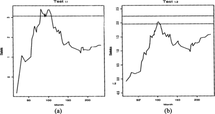
Note that using the statistics process of Test 1.2 with varying n, only the scale on the vertical axis would change. The reason why Test 1.2 is not significant is that the weight function makes it difficult to pick up differences in treatments early in the process, and at the end of the study H ₀ cannot be rejected based on the complete data. If we use 12 years of data, as in Slud and Wei's paper, with a 3-year inspection design, then only n = 48 observations are available, and with n = 50 the two-sided Test 1.2 would be significant in the period 93–111 months.

Example 2.2

George et al. (1994) describe in detail the results of the comparison of two treatments of lung cancer patients from Cancer and Leukemia Group B (CALGB) data: radiotherapy alone (A) or chemotherapy followed by radiotherapy (B). The trial was modified from the original fixed-sample-size design to allow interim analyses, and it was stopped after 34 months, earlier than planned, due to a significant result in favor or treatment (B). As the details of the implementation of Lan and DeMets's (1983) α-spending function are not given in George et al. (1994), we reanalyzed the data using the O'Brien-Fleming method with 7 analyses (one evaluation per six months). The critical values were taken from Jennison and Turnbull (2000), and they give significant result at month 34, as in George et al. (1994). Figure 2 shows the statistics process of the available data if the time unit is rounded to months. For Test 1.1, the α = 0.1 critical level is included in the graph. It shows that at α = 0.05 the two-sided test is not significant, but the α = 0.1 line is crossed, giving weak evidence to some treatment difference. This is in fact supporting the final conclusion.

Figure 2 CALGB data: (a) Test 1.1 with C ₁(0.1, 150) = 2.89; (b) Test 1.2 with n = 111 and .

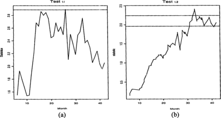
For Test 1.2 the statistics values have to be rescaled with a factor k/n at the time of the kth observed event. Using the three and a half years as the conclusion of the study, by which time n = 111 events have been observed, at α = 0.05 Test 1.2 would have indicated difference in treatment in the 33rd month. The process is not significant before or after this month. We note that the last analysis in the above O'Brien–Fleming test in not significant either. So, in all, we conclude that although at some point the α = 0.05 significance level is reached by these tests using the weight function q(u) = 1, the retrospective analysis shows that the difference is not very great. This was the conclusion of the original paper, where the treatment difference was estimated. We note that the one-sided α = 0.05 boundary would have been crossed in months 31–42 in the sequential trial using Test 1.3.

In such marginal cases continuous monitoring gives added insight into the nature of the difference, as the statistic value is given not only at some discrete points, but continuously.

3. CONCLUSIONS

We have defined new algorithms for continuous monitoring of data in clinical trials when the problem of interest is to decide if there is any difference between two treatments. These tests are fully sequential versions of the currently used group sequential tests, and hence allow complete flexibility in scheduling the evaluation of evidence. They are computationally much more simple than the currently used approach using α-spending functions. Fully sequential procedures can stop earlier than the group sequential versions. We also demonstrated that the complete statistics process gives more information about the phenomenon under study than the discrete monitoring version where the statistics are calculated at some selected time points only.

ACKNOWLEDGMENTS

This research was supported in part by an NSERC Canada operating grant. Data for the second example was most generously provided by Professor M. R. Sooriyarachchi of the University of Colombo, Sri Lanka.

Notes

Recommended by N. Mukhopadhyay

APPENDIX

We assume that the null hypothesis of no difference between the two treatments is true.

We can write V(t) = ∑ _i x _i (t), where . By our assumptions, x _i (t), i ≥ 1, are independent, but not identically distributed. However, in the sum V(t), only terms with Δ _i (t) = 1 contribute, and for these terms X _i (t) = X _i (∞), N _i (X _i (t), t) = 1, if t ≥ inf _u Δ _i (u) = 1. Hence we can use the classical theorems for approximating independent and identically distributed random variable sums by a Brownian motion. It is easy to see that the conditions for the terms in Komlós et al. (1975); Komlós et al. (1976) are satisfied.

Lemma 2.4 of Slud (1984) has proven that R(t) for 0 < t ≤ t _j is, uniformly in t, stochastically smaller than a random variable with mean zero and variance O(log j).

From this

First consider weight function q(u) = u ^1/2. We have from (A.1) that

From (1.3) it follows that the critical value is O((log log n)^1/2) in Test 1.1, and hence the weighted error term is negligible for large n.

For weight functions q(u), 0 < u < 1, if q(u) = u ^Δ, 0 ≤ Δ < 1/2, the negligibility of the weighted error term follows directly from (A.1).

REFERENCES

- Csörgo , M. , Shao , Q. M. , and Szyszkowicz , B. ( 1991 ). A Note on Local and Global Functions of a Wiener Process and Some Rényi Statistics , Studia Scientiarum Mathematicarum Hungarica 26 : 239 – 259 .
- Darling , D. A. and Erdős , P. ( 1956 ). A Limit Theorem for the Maximum of Normalized Sums of Independent Random Variables , Duke Mathematical Journal 23 : 143 – 145 .
- George , S. L. , Li , C. , Berry , D. A. , and Green , M. R. ( 1994 ). Stopping a Clinical Trial Early: Frequentist and Bayesian Approaches Applied to a CALGB Trial in Non-small-cell Lung Cancer , Statistics in Medicine 13 : 1313 – 1327 .
- Gombay , E. ( 1996 ). The Weighted Sequential Likelihood Ratio , Canadian Journal of Statistics 24 : 229 – 239 .
- Gombay , E. ( 2002 ). Parametric: Sequential Tests in the Presence of Nuisance Parameters , Theory of Stochastic Processes 8 : 107 – 118 .
- Gombay , E. and Hussein , A. A. ( 2006 ). Sequential Comparison of Two Populations by Parametric Tests , Canadian Journal of Statistics 34 : 217 – 232 .
- Jennison , C. and Turnbull , B. W. ( 2000 ). Group Sequential Methods with Applications to Clinical Trials , Boca Raton : Chapman Hall/CRC .
- Komlós , J. , Major , P. , and Tusnády , G. ( 1975 ). An Approximation of Partial Sums of Independent R.V.'s and the Sample DF. I , Zeitschrift für Wahrscheinlichkeitstheorie und verwandte Gebiete 32 : 111 – 131 .
- Komlós , J. , Major , P. , and Tusnády , G. ( 1976 ). An Approximation of Partial Sums of Independent R.V.'s and the Sample DF. II , Zeitschrift fur Wahrscheinlichkeitstheorie und verwandte Gebiete 34 : 33 – 58 .
- Lan , K. K. G. and DeMets , D. L. ( 1983 ). Discrete Sequential Boundaries for Clinical Trials , Biometrika 70 : 659 – 663 .
- O'Brien , P. C. and Fleming , T. R. ( 1979 ). A Multiple Testing Procedure for Clinical Trials , Biometrics 35 : 549 – 556 .
- Pocock , S. J. ( 1977 ). Group Sequential Methods in the Design and Analysis of Clinical Trials , Biometrika 64 : 191 – 199 .
- Slud , E. V. ( 1984 ). Sequential Linear Rank Tests for Two-Sample Censored Survival Data , Annals of Statistics 12 : 551 – 557 .
- Tsiatis , A. A. ( 1982 ). Repeated Significance Testing for a General Class of Statistics Used in Censored Survival Analysis , Journal of American Statistical Association 77 : 855 – 861 .
- Vostrikova , L. J. ( 1981 ). Detection of a “Disorder” in a Wiener Process , Theory of Probability and Its Applications 26 : 356 – 362 .
- Wang , S. K. and Tsiatis , A. A. ( 1987 ). Approximately Optimal One-Parameter Boundaries for Group Sequential Trials , Biometrics 43 : 193 – 199 .