Economically challenged and water scarce: identification of global populations most vulnerable to water crises

ABSTRACT

The best available high-resolution precipitation, GDP, available freshwater and withdrawal data sets are used in a combined global analysis of physical and economic water scarcity at 50 km resolution. We find that approximately 40.7 million people are living in areas with concurrent severe economic and water-scarcity constraints. These areas are mostly in semi-arid parts of Sub-Saharan Africa, the Middle East and Central Asia.

KEYWORDS:

• Water stress
• available freshwater resources
• water withdrawals
• GDP
• virtual water trade
• grid analysis

View correction statement:

Correction

Introduction

Water is one of the most important resources in the world, if not the most important. Water is needed and used for practically everything, from household domestic use to industrial and agricultural production. Even though over 70% of the Earth’s surface is covered by water, only a small fraction of Earth’s water is viable for supply due to its great heterogeneity in space and time (Oki & Kanae, 2006). Water scarcity is broadly the consequence of the spatial distribution of population growth relative to available water resources (Kummu et al., 2016). More often than not, infrastructure to harvest and manage water supplies cannot keep up with the steadily growing demand. Varis, Biswas, Tortajada, and Lundqvist (2006) outlined the water management problems faced by several developing megacities around the world, citing unprecedented population growth and poor infrastructure planning as two of the common causes of water stress. To make things worse, climate change has altered natural hydrological patterns. There is a systematic increase in the variance of precipitation around the world over the last few decades; wet areas are becoming wetter, and dry and arid areas drier (Dore, 2005). Big cities all over the world are now experiencing recurring water shortages. Sao Paulo in Brazil, Jakarta in Indonesia, Bangalore in India and Cape Town in South Africa are just some of the cities that recently made international headlines due to water shortages.

By definition, water scarcity is a general state of water insufficiency. Water stress is defined as a state when certain threshold values are exceeded (Hanasaki, Yoshikawa, Pokhrel, & Kanae, 2018a). Water scarcity was further classified by Rijsberman (2006) into two different types: physical and economic. Physical water scarcity is the insufficiency or lack of water itself. This type of scarcity is often found in arid regions. Economic water scarcity is an insufficiency of water associated with lack of capacity to use water resources despite its availability or abundance. Economic water scarcity is often associated with inadequate infrastructure development and poor management, as well as cases of inequitable water allocation and access across economic levels. Access to safe drinking water tends to improve with economic growth. The achievement of the Millennium Development Goal for drinking water (Target 7-C) was associated with the rapid economic growth in China and India in 1990–2015 (Fukuda, Noda, & Oki, 2019).

Although supply and demand are the fundamental factors dictating water stress, economic forces interfere and alter the dynamics of these two. Standard of living changes water use behaviours; richer economies tend to use more water per capita. On the supply side, the capacity for building utility infrastructure also correlates with economic stature. Inter-basin transfers, groundwater extraction and seawater desalination are just some of the common alternatives to conventional water supply, which are all undeniably capital-intensive. Also, the urbanization process, along with the distribution and growth of population in megacities, is different in developed and developing economies (Biswas, 2004). Megacities in developing countries grow exponentially faster than their developed and industrialized counterparts. But the magnitude of economic development is concurrent with population growth only in industrialized cities, leaving developing cities behind (Varis et al., 2006). The importance of water resource management in alleviating water stress, especially in cases of economic water scarcity in developing countries, was highlighted by Biswas and Tortajada (2010a, 2010b). In their case study of Phnom Pehn, Cambodia, the drastic improvement in public access to water since institutional restructuring has demonstrated that effective leadership and governance can alleviate water scarcity (Biswas & Tortajada, 2010b).

Historically, water scarcity has been quantified by a multitude of indicators. Liu et al. (2017) provided a comprehensive summary of water stress indicators categorized into five classes. Among them, the indicators most widely used are the withdrawal-to-availability ratio, also commonly known as the withdrawal-to-water ratio (WWR), and availability per capita (APC). These indicators have their own respective classifications of scarcity levels. Hanasaki et al. (2018a) briefly discussed the development processes and the supporting evidence for these thresholds for both indicators, which were both primarily obtained empirically using several case studies and approximations.

Oki, Yano, and Hanasaki (2017) discussed the relationship among physical water scarcity expressed by APC, gross domestic product (GDP), and the export/import quantity of virtual water trade through major crops based on country-level analysis. They found that most of the net virtual water exporting countries have higher APC than the net virtual water importing countries, and moreover, there is no country with low APC and low GDP. The analysis suggests that a country can survive with little money provided that it has enough water to grow crops to feed itself, and even a water-scarce country can survive if it has the purchasing power to import necessary food from abroad or engineer additional water supply domestically. But countries facing both economic hardship and water scarcity cannot support their basic needs over the long term, so they do not exist in the contemporary world. This result implies that we need to consider both the physical and the economic water scarcity of a region to determine whether the region is truly in distress, with chronic water shortage.

In this study, we jointly analyze the physical and economic water scarcity of the world at 50 km resolution, in an extension of the precursor analysis by Oki et al. (2017). We illustrate the current state of global freshwater resources, and pinpoint the areas and populations at greatest risk of a water crisis.

Data

Table 1 summarizes the gridded data sets collected and used for this study, with particulars such as spatial resolution, units and variables. A brief explanation of the data sources and assumptions for each follows.

Table 1. Data used in this study

Parameter	Variable	Unit and Size	Source
GDP-PPP (0.5° × 0.5°)	GDP in 2020	USD billions per year	Murakami and Yamagata (2016)
Precipitation (0.01° × 0.01°)	Mean annual precipitation	mm/y	Karger et al. (2017)
Population (0.5° × 0.5°)	Population	capita per grid	Goldewijk, Beusen, Doelman, and Stehfest (2017)
Available freshwater (0.5° × 0.5°)	Total Runoff total (surface + subsurface)	kg/m^2/s	Hanasaki et al. (2018a)
Withdrawal rate (0.5° × 0.5°)	Net industrial water consumption	kg/m^2/s
	Net domestic water withdrawal
	Net agricultural water withdrawal

The GDP data set is from the Japan Center for Global Environmental Research, National Institute for Environmental Studies (Murakami & Yamagata, 2016). GDP was estimated by downscaling projected country population under different socio-economic pathways. SSP2 (the ‘middle of the road’ shared socioeconomic pathway) was used, in which the world population will peak early in the latter half of the twenty-first century (Takakura et al., 2019).

Climatological mean precipitation data are from Climatologies at High Resolution for the Earth Land Surface Areas (CHELSA; Karger et al., 2017). CHELSA is an organization hosted by the Swiss Federal Institute for Forest, Snow and Landscape Research WSL. The 0.01 × 0.01 degree data set was constructed using data from 1979 to 2013.

The gridded data sets of available freshwater and withdrawals were produced using the global hydrological model called H08 (Hanasaki et al., 2008, 2018a). This is a grid-cell-based model of global hydrology and world water resources, consisting of six submodels, including human interventions such as storage in and releases from artificial reservoirs and irrigation withdrawals, coupled with a crop growth model. The model was run in accordance with the ISIMIP2b protocol (Frieler et al., 2017). ISIMIP (the Inter-sectoral Impact Model Intercomparison Project, www.isimip.org) offers a framework and protocols for different modellers in projecting the impacts of climate change. Available freshwater was estimated as total runoff, the sum of surface and subsurface runoff components. Domestic, industrial and agricultural withdrawals were also obtained from the estimates of H08 (Hanasaki, Yoshikawa, Pokhel, & Kanae, 2018b). Net withdrawal was set to be the sum of these three withdrawals. To be consistent, the population information provided for ISIMIP2b (Goldewijk et al., 2017) was also used. The precipitation information in ISIMIP2b is not from CHELSEA but based on various other sources.

Results

The distribution of population across the globe is uneven. A study by the United Nations found that the global urban population had exceeded the global rural population for the first time in 2007 (UNFPA, 2007). As of 2011, there were more than 3.6 billion people living in urban areas, and this number is projected to increase by another 2.6 billion by 2050 (UN, 2012).

Statistically, approximately 45% of earth’s land is practically uninhabited, with less than one capita per square kilometre (Figure A1 in the online supplemental material). Sixty per cent of the world’s 7.7 billion people live on only 9% of the land area.

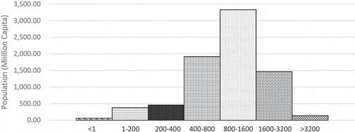
Precipitation is concentrated in equatorial regions and coastal areas (Figure A2). The desert regions of North Africa and the Middle East are easily recognizable due to their low precipitation. People mostly live in areas with mean annual precipitation of 800–1600 mm/y, followed by 400–800 mm/y and 1600–3200 mm/y (Figure 1).

Figure 1. Histogram of population in terms of mean annual precipitation (mm/year).

Figure 2 is based on the estimated global distribution of precipitation (Figure A2) cross-referenced with the global distribution of population (Figure A1) and shows the available precipitation water per capita per year. To avoid extreme magnification in the areas with very low population density, the minimum population density was set to one capita per square kilometre; areas with lower population density (indicated by grey shading) were excluded from further analysis.

Figure 2. Histogram of population in terms of available precipitation water (m3/capita/year).

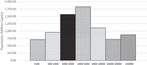
Large areas in most of the continents have more than 20,000 m³ per capita per year of available precipitation water (Figure A3), and only limited areas of Europe, South Asia, North Africa, the Middle East, South Asia and East Asia have less than 1000 m³ per capita per year. The histogram is highest in the range of 2000–5000 m³ per capita per year, followed by 1000–2000 m³ per capita per year and 5000–10,000 m³ per capita per year. But more than 600 million people live in the other ranges. For example, more than 800 million live in areas with more than 20,000 m³ per capita per year.

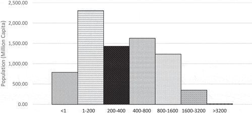
In general, available freshwater (Figure A4) is lower than precipitation (Figure A2). Of the more than 60,000 land grid boxes (excluding Antarctica), approximately 3000 have more runoff than precipitation, due to the runoff from additional irrigation water internally calculated in H08. The histogram of population in terms of annual runoff (Figure 3) is highest in the range of 1–200 mm/y, but similar for 200–400, 400–800 and 800–1600 mm/y. Due to the nonlinear conversion of precipitation into runoff, Figures 1 and 3 show different distributions.

Figure 3. Histogram of population in terms of annual runoff (mm/year).

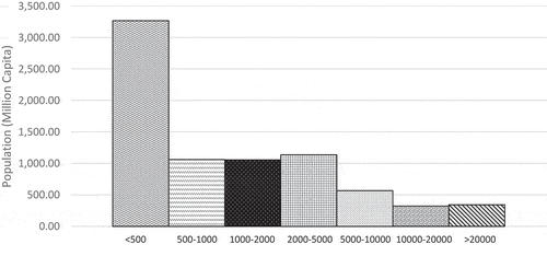
The global distribution of available freshwater per capita is shown in Figure 4. As with Figure A3, a large fraction of Earth’s land masses have more than 20,000 m³ per capita per year of available freshwater. At the same time, semi-arid regions in Sub-Saharan Africa, large areas of Eastern Europe, and some parts of south-eastern China have less than 1000 m³ per capita per year. Large tracts of northern and eastern Africa, the Middle East, West Asia and some parts of South and East Asia have even less – under 500 m³ per capita per year. Aproximately half of the world’s population lives in areas in this category (Figure 5). Figures 3 and 5 suggest that population density tends to be higher in areas where more freshwater is available.

Figure 4. Spatial distribution of available freshwater (m³/capita/year).

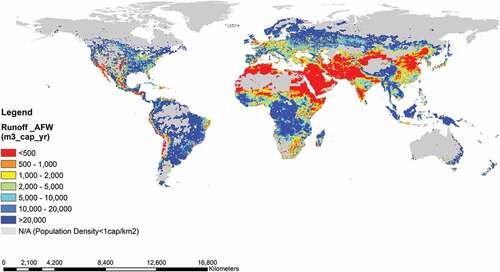
Figure 5. Histogram of population in terms of available freshwater (m³/capita/year).

Based on these estimates, water-stress conditions can be inferred using the indicator and threshold values of Shiklomanov (1997) for available freshwater. Table 2 summarizes the ratio of population in each category of water scarcity assessed by APC, with available precipitation water per capita for comparison.

Table 2. Distribution of population by water availability

Availability (m^3 per capita per year)	Description	Population distribution (%)
		Rainwater	Freshwater
<500	Extremely low	9.2	42.2
500–1000		12.3	13.7
1,000–2,000	Very low	20.2	13.6
2,000–5,000	Low	23.6	14.7
>5,000	Average	34.8	15.9

Water stress is fundamentally driven by two factors: supply and demand. Although water availability in terms of m³ per capita per year, as summarized in Table 2, can provide a good estimate of water stress, this assumes that per capita demand is similar throughout the global population. But studies (FAO, 2016) have shown that per capita consumption varies across countries and regions, often affected by different factors, such as culture, climate and lifestyle (Akuoko-Asibey, Nkemdirim, & Draper, 1993; Khadam, 1988).

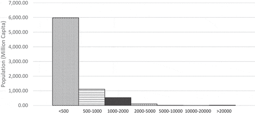
Withdrawal and consumption can be divided into several sectors. In this study, net withdrawal is taken to be the sum of agricultural, industrial and domestic water withdrawals. The spatial distribution of sectoral withdrawals is shown in Figures A5–A8 for agricultural, industrial, domestic and total withdrawals, respectively.

The global agricultural water requirement is the highest in these three sectors, with net annual requirements of 1607 km³ (Figure A5). Despite being the largest component, the spatial distribution of irrigation withdrawal is highly concentrated in certain regions, such as southern and eastern Asia. With 1050 km³/y, industrial withdrawal (Figure A6) comes in second. Domestic withdrawal is estimated as 377 km³/y (Figure A7). Aggregating these sectoral withdrawals gives 3,034 km³ global annual net withdrawals (Figure A8). Considering the population distribution, nearly 6 billion of the world’s people use less water than 500 m³ per capita per year (Figure 6).

Figure 6. Histogram of population in terms of net total annual withdrawal (m³/capita/year).

It should be restated that some of the water withdrawals, particularly for agricultural and industrial water, are for external consumption in addition to local consumption, as expressed by the concept of ‘virtual water trade’ (Allan, 1998; Oki & Kanae, 2004).

Using the distribution of availability (Figure 4) and net total withdrawals (Figure A8), the unit-less indicator of water scarcity, WWR, can be estimated as

(1) $WWR=W/Q$(1)

where W is the annual water withdrawal and Q is the annual runoff/available freshwater. The geographical distribution of WWR is presented in Figure 7.

Figure 7. Spatial distribution of water stress represented by withdrawal-to-available-water ratio (WWR).

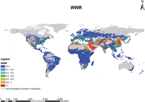
Raskin, Gleick, Kirshen, Pontius, and Strzepek (1997) suggest that when WWR is below 0.1, the region is classified as having no water stress, 0.1–0.2 is low water stress, 0.2–0.4 is moderate water stress, and over 0.4 is high water stress. Following this classification, the distribution of population with respect to water stress is summarized in Table 3 and Figure 8.

Table 3. Distribution of population by water stress

Withdrawal-to-available-water ratio	Remarks	Population distribution (%)
			<0.1	No water stress	81.8
0.1–0.2	Low water stress	6.2
0.2–0.4	Moderate water stress	4.6
>0.4	High water stress	7.5

Figure 8. Histogram of population in terms of withdrawal-to-available-water ratio.

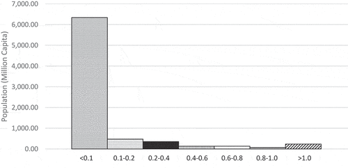
Although both APC (Table 2) and WWR (Table 3) are indicators intended to quantify water stress, they cannot be directly compared. If we compare the fraction of the most water stressed population, there is a considerable difference between these indicators. In Table 2, more than half of the world’s population (55.9%, 4.3 billion) have extremely or catastrophically low water availability. But in Table 3, only 7.5% (582 million) are in high-water-stress conditions. This apparent discrepancy may be partly explained by the fact that return flow, or unconsumed water withdrawals that are returned to the natural system, are excluded from the analysis. Recall that net water withdrawal is considered in this study. Consequently, the water withdrawal in this study is much smaller than conventional water withdrawals, by approximately one-half for agricultural water withdrawals for example, and the WWR in Table 3 may be underestimated.

GDP is commonly used to quantify economic activity. Figure A9 shows the spatial distribution of GDP per capita (based on purchasing power parity, PPP) in USD in 2005.

Figure 9 is a scatter plot (log-log scale) of GDP-PPP per capita versus APC. The size of each circles indicates the population count. Oki et al. (2017) found that there are no countries that are both economically challenged and under water scarcity, as would be denoted by lying below the dashed thick line (connecting USD 10,000 of GDP-PPP per capita and 10,000 m³ of available freshwater per capita per year). No country was found below the threshold line, but some 0.5° grid points do fall below that line in this study. This could be caused by the heterogeneity of water and monetary resources within nations.

Figure 9. Scatter plot of water availability per capita and GDP-PPP per capita analyzed by 0.5° longitudinal and latitudinal grid boxes.

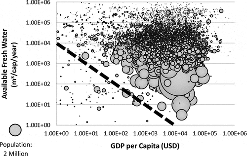
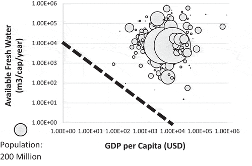
To check for consistency between the analysis of Oki et al. (2017) and our current study, the gridded data for water APC and GDP-PPP per capita were averaged in each nation (Figure 10). This is very similar to Oki et al.’s (2017) country-level analysis, and the population that is both economically challenged and water stressed can be only delineated in a finer-mesh analysis (Figure 9).

Figure 10. Scatter plot of water availability and GDP-PPP per capita by country-level analysis.

Finally, the grid boxes below the threshold line (connecting USD 10,000 of GDP-PPP per capita and 10,000 m³ of available freshwater per capita per year), corresponding to regions with a perilous combination of low GDP per capita and water scarcity, are presented in Figure 11. Such areas are located in parts of northern and eastern Africa, the Middle East, West Asia, and central to north-eastern Asia. People in these regions are at great risk because they experience shortages of available freshwater to grow food, and also have difficulty purchasing food due to lack of economic power. Of the 40.7 million people living in these areas prone to water crises, approximately 10.2 million are living in areas with WWR of 0.4 or more, and 30.5 million in areas with WWR less than 0.4. These results suggest that more comprehensive assessments of water scarcity will be possible using multiple numerical indicators (Falkenmark, Lundqvist, & Widstrand, 1989).

Figure 11. Longitudinal and latitudinal grid boxes (0.5° × 0.5°) showing areas below the threshold line of both economically poor and water-scarce.

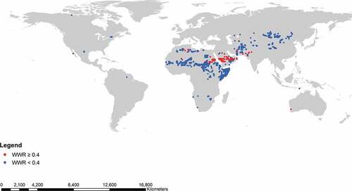
There are identified grid boxes near Mexico City and Perth in Western Australia in Figure 11, as well. These could be due to the inconsistency between the downscaled population and GDP data used in this study, even though these regions are known to be seriously water stressed; for example, a seawater desalination plant was built near Perth and started operation in 2006.

This study excludes the explicit considerations of various factors affecting physical water scarcity, such as seasonality, interannual variability, groundwater supplies, water quality and hydropower demands, which have been already considered in some pioneering studies (Hanasaki et al., 2018a; Wada et al., 2017). Further integration of socio-economic aspects in modern assessments of world water resources is expected.

Conclusion

Even though annual precipitation and annual runoff have high spatial heterogeneity, most people live in areas with 400–3200 mm/y of precipitation and less than 500 m³ per capita per year of available freshwater. Net total annual withdrawal is also less than 500 m³ per capita per year for nearly 6 billion people, and a similar number of people live in areas with a net withdrawal-to-availability ratio less than 0.1. Combined analysis of physical and economic water scarcity, for the first time ever, shows that some regions in the world, analyzed by 0.5° longitudinal and latitudinal grid boxes, are below the threshold line connecting the USD 10,000 per capita per year of GDP and 10,000 m³ per capita per year of available freshwater recourses, and they are mostly in northern and eastern Africa, the Middle East, West Asia, and central to north-eastern Asia, with a total current combined population of approximately 40.7 million. People in such regions should have support from outside the region in the same nation, or from outside the nation, since they may have not enough water to grow food internally, and not enough purchasing power to compensate for water shortage by importing food.

These results depend on the spatial scale used in the analysis, as illustrated by Oki et al. (2001), and we would be able to differentiate more acute but limited areas of economically challenging and water-scarce regions from the majority of less water-scarce regions, if we had finer-scale information over the globe. But the proposed methodology to identify the regions with chronic water shortage due to economic and hydrological reasons should be useful to develop and implement countermeasures. Projections of future water crisis potential could be achieved by applying the approach used here to future GDP and water availability estimates (e.g. Ferguson, Pan, & Oki, 2018).

Acknowledgments

The authors thank Dr C. R. Ferguson of the University at Albany, SUNY, for his support to finalize the draft. The first author feels great honour and acknowledges Dr Asit Biswas for his generous offer to accept this work for his Festschrift, because Dr Biswas has been a mentor on the fundamental issues of how we should tackle and understand world water issues, and develop and propose policy-relevant solutions, for more than two decades, since the Next Generation Water Leaders programme, which Dr Biswas organized with the Nippon Foundation and prepared for the 2nd World Water Forum in 2000.

Disclosure statement

No potential conflict of interest was reported by the authors.

Supplementary Material

Supplemental data for this article can be accessed at https://doi.org/10.1080/07900627.2019.1698413.

Additional information

Funding

This work was supported by the Japan Society for the Promotion of Science [KAKENHI; 16H06291].

References

- Akuoko-Asibey, A., Nkemdirim, L. C., & Draper, D. L. (1993). The impacts of climatic variables on seasonal water consumption in Calgary, Alberta. Canadian Water Resources Journal/Revue canadienne des ressources hydriques, 18(2), 107–116. doi:10.4296/cwrj1802107
- Allan, J. A. (1998). Virtual water: A strategic resource, global solution to regional deficits. Groundwater, 36(4), 545–546. doi:10.1111/j.1745-6584.1998.tb02825.x
- Biswas, A. (2004). Integrated Water Resources Management: A reassessment. A Water Forum contribution. Water International, 29(2), 248–256. doi:10.1080/02508060408691775
- Biswas, A., & Tortajada, C. (2010a). Future water governance: Problems and perspectives. Water Resources Development, 26(2), 129–139. doi:10.1080/07900627.2010.488853
- Biswas, A., & Tortajada, C. (2010b). Water supply of Phnom Penh: An example of good governance. Water Resources Development, 26(2), 157–172. doi:10.1080/07900621003768859
- Dore, M. (2005). Climate change and changes in global precipitation patterns: What do we know? Environment International, 31(8), 1167–1181. doi:10.1016/j.envint.2005.03.004
- Falkenmark, M., Lundqvist, J., & Widstrand, C. (1989). Macro-scale water scarcity requires micro-scale approaches: Aspects of vulnerability in semi-arid development. Natural Resources Forum, 13(4), 258–267. doi:10.1111/narf.1989.13.issue-4
- Ferguson, C. R., Pan, M., & Oki, T. (2018). The effect of global warming on future water availability: CMIP5 synthesis. Water Resources Research, 54, 7791–7819. doi:10.1029/2018WR022792
- Food and Agriculture Organization of the United Nations (FAO). (2016). AQUASTAT main database. Retrieved from http://www.fao.org/nr/water/aquastat/data/query/
- Frieler, K., Lange, S., Piontek, F., Reyer, C. P. O., Schewe, J., Warszawski, L., … Yamagata, Y. (2017). Assessing the impacts of 1.5°C global warming: Simulation protocol of the Inter-Sectoral Impact Model Intercomparison Project (ISIMIP2b). Geoscientific Model Development, 10, 4321–4345. doi:10.5194/gmd-10-4321-2017
- Fukuda, S., Noda, K., & Oki, T. (2019). How global targets on drinking water were developed and achieved. Nature Sustainability, 2, 429–434. doi:10.1038/s41893-019-0269-3
- Goldewijk, K., Beusen, A., Doelman, J., & Stehfest, E. (2017). Anthropogenic land use estimates for the Holocene: HYDE 3.2. Earth System Science Data, 9, 927–953. doi:10.5194/essd-9-927-2017
- Hanasaki, N., Kanae, S., Oki, T., Masuda, K., Motoya, K., Shirakawa, N., … Tanaka, K. (2008). An integrated model for the assessment of global water resources, Part 2: Applications and assessments. Hydrology and Earth System Sciences, 12, 1027–1037. Retrieved from www.hydrol-earth-syst-sci.net/12/1027/2008/
- Hanasaki, N., Yoshikawa, S., Pokhrel, Y., & Kanae, S. (2018a). A quantitative investigation of the thresholds for two conventional water scarcity indicators using a state-of-the-art global hydrological model with human activities. Water Resources Research, 54, 8279–8294. doi:10.1029/2018WR022931
- Hanasaki, N., Yoshikawa, S., Pokhel, Y., & Kanae, S. (2018b). A global hydrological simulation to specify the sources of water used by humans. Hydrology and Earth System Sciences, 22, 789–817. doi:10.5194/hess-22-789-2018
- Karger, D. N., Conrad, O., Böhner, J., Kawohl, T., Kreft, H., Soria-Auza, R. W., … Kessler, M. (2017). Climatologies at high resolution for the earth’s land surface areas. Scientific Data, 4, 170122. doi:10.1038/sdata.2017.122
- Khadam, M. A. A. (1988). Factors influencing per capita water consumption in urban areas of developing countries and their implications for management, with special reference to the Khartoum metropolitan area. Water International, 15(5), 226–229. doi:10.1080/02508068808687095
- Kummu, M., Guillaume, J. H. A., de Moel, H., Eisner, S., Ward, P. J., & de Moel, H. (2016). The world’s road to water scarcity: Shortage and stress in the 20th century and pathways towards sustainability. Scientific Reports, 6, 38495. doi:10.1038/srep38495
- Liu, J., Yang, H., Gosling, S. N., Kummu, M., Flörke, M., Pfister, S., ... Oki, T. (2017). Water scarcity assessments in the past, present, and future. Earth’s Future, 5(6), 545–559. doi:10.1002/2016EF000518
- Murakami, D., & Yamagata, Y. (2016). Estimation of gridded population and GDP scenarios with spatially explicit statistical downscaling. ArXiv. Retrieved from https://arxiv.org/abs/1610.09041
- Oki, T., Agata, Y., Kanae, S., Sarushi, T., D., Y., & Musiake, K. (2001). Global assessment of current water resources using total runoff integrating pathways. Hydrological Science-Journal-des Science Hydrologiques, 46, 983–995. doi:10.1080/02626660109492890
- Oki, T., & Kanae, S. (2004). Virtual water trade and world water resources. Water Science and Technology, 49(7), 203–209. doi:10.2166/wst.2004.0456
- Oki, T., & Kanae, S. (2006). Global hydrological cycles and world water resources. Science, 313, 1068–1072. doi:10.1126/science.1128845
- Oki, T., Yano, S., & Hanasaki, N. (2017). Economics of virtual water trade. Environmental Research Letters, 12, 044002. doi:10.1088/1748-9326/aa625f
- Raskin, P., Gleick, P., Kirshen, P., Pontius, G., & Strzepek, K. (1997). Comprehensive assessment of the freshwater resources of the world. Stockholm, Sweden: Stockholm Environment Institute.
- Rijsberman, F. R. (2006). Water scarcity: Fact or fiction? Agricultural Water Management, 80, 5–22. doi:10.1016/j.agwat.2005.07.001
- Shiklomanov, I. A. (1997). Assessment of water resources and water availability in the world (pp. 88). Geneva: SEI and WMO.
- Takakura, J., Fujimori, S., Hanasaki, N., Hasegawa, T., Hirabayashi, Y., Honda, Y., … Hijioka, Y. (2019). Dependence of economic impacts of climate change on anthropogenically directed pathways. Nature Climate Change, 9, 737–741. doi:10.1038/s41558-019-0578-6
- UNFPA. (2007). State of world population 2007: Unleashing the potential of urban growth. New York: UNFPA. doi:10.18356/fe74b223-en
- United Nations (UN). (2012): World urbanization prospects: The 2011 Revision. New York: UN.
- Varis, O., Biswas, A., Tortajada, C., & Lundqvist, J. (2006). Megacities and water management. Water Resources Development, 22(2), 377–394. doi:10.1080/07900620600684550
- Wada, Y., Bierkens, M. F. P., de Roo, A., Dirmeyer, P. A., Famiglietti, J. S., Hanasaki, N., … Wheater, H. (2017). Human-water interface in hydrological modeling: Current status and future directions. Hydrology and Earth System Sciences, 21, 4169–4193. doi:10.5194/hess-21-4169-2017