Improving opinion poll reporting: the Irish Polling Indicator

ABSTRACT

This article describes a statistical method for aggregating the information from Irish opinion polls. Such aggregate estimates provide academic researchers with a time series of support for political parties, and inform the public better about opinion polls by focusing on trends and uncertainty in these estimates. The article discusses the challenge of aggregating opinion polls in a multi-party setting with a comparatively limited number of polls available and presents daily estimates of party support for the 1987–2016 period. The article develops a method to better model major sudden political and societal events, which have been common in Ireland since 2007. Finally, it discusses how polling aggregation estimates can enhance opinion poll reporting in the media.

KEYWORDS:

• Opinion polls
• Ireland
• public opinion

Perhaps more than ever, opinion polls shape election campaigns (van der Meer et al., 2015). Journalists use polls to determine what and who to focus on. Parties use them to help sell their message to voters. And voters rely on them for strategic voting (Lago et al., 2015). Opinion polls regarding the relative strength of each party take particular prominence, even outside of election campaigns. Advances in phone and internet polling mean that more and more polls are available. In Ireland, the two long-standing pollsters Ipsos MRBI and Millward Brown have been joined by Red C Research and, more recently, Behaviour & Attitudes. Since 2011, an average of just over two opinion polls per month has been published, most of which received considerable attention in newspapers and on television.

More opinion polls do not automatically imply better information for the public, journalists, parties and researchers. Pollsters use different approaches and are therefore likely to report differing results, not just due to random sampling error, but systematic, long-term differences due to design choices. This paper describes the Irish Polling Indicator, a method for aggregating the information contained in opinion polls, taking into account both random error and systematic differences between the polls. It builds on earlier work in, among others, Australia, Canada, Germany and the United Kingdom (Jackman, 2005; Fisher et al., 2011; Cantu et al., 2015; Walther, 2015; Hanretty et al., 2016) and extends this to the Irish case, which has a comparatively high number of political parties (compared to Canada and Australia) and a relatively modest volume of polls (compared to the United Kingdom). In addition, the paper discusses how major events that arguably shock public opinion can be better incorporated into poll aggregation models. This is particularly relevant for the Irish case, which has seen major economic challenges that affected people's party preferences at short notice.

The aim of the Irish Polling Indicator is twofold. First of all, by aggregating opinion polls for each parliamentary term it provides a historical time series of party support that can be used in political research. While in anecdotal accounts of election campaigns and governance, opinion polls seem to play a regular role, political scientists have relatively recently begun to look at their impact on policy-making in a more structural fashion (Hobolt and Klemmensen, 2008; Soroka and Wlezien, 2010; Pickup and Hobolt, 2015). While opinion poll data are available for Ireland, it is somewhat scattered and concerns individual polls only (Marsh, 2006; ISSDA, 2015). Existing approaches to pooling opinion polls have focused on campaign polls only (McElroy and Marsh, 2008). Secondly, opinion polls are regularly reported in news media, with strong conclusions based on non-significant poll changes featuring all too often. Poll aggregation makes systematic differences between polling companies visible and stresses the uncertainty associated with these estimates.

1. Two types of error in opinion polls

Opinion polls are a classic example of using a sample to learn something about a population. We are not interested in the political views of 1000 randomly selected individuals as such, but we ask them for their opinions as this can tell us something about the beliefs of the whole population. This does not mean that every sample will be exactly reflective of the population, as any introductory text on statistics will point out. Often two types of error are distinguished: random and systematic error (King et al., 1994: 63).

Random error varies between samples drawn from the same population. An important source of random error is sampling error. Because Irish opinion polls are usually limited to around 1000 randomly selected people we might, just by chance, encounter a higher percentage of Fine Gael voters among our thousand than there are in the population as a whole. If we would repeat the sampling procedure the random error is likely to be somewhat different. When using simple random sampling, the size of this source of error is known, or to put it better: the Central Limit Theorem informs us that the sampling distribution will be approximately normal. Sampling error is often presented as the sole source of error in the polls (‘the margin of error’), but it only covers only random error due to sampling. Moreover, the usual equations for calculating random error are only valid when each member of the population has an equal chance of being sampled and these probabilities are independent. The Irish pollsters that use face-to-face interviewing generally limit the number of physical locations of fieldwork (‘sampling points’) to 64 (Millward Brown), 100–125 (Behaviour & Attitudes) or 120 (Ipsos), interviewing between 10 and 15 people in each location.¹ In the past, the number of sampling points was lower (and the number of interview per location higher). This introduces clustering in the sample and without correction the standard errors of estimated statistics will be underestimated (Kish, 1957; Arceneaux and Nickerson, 2009). On the other hand, post-stratification can reduce the standard error, especially if the weighting variables are strongly related to the variable of interest. For example, if we know that women are more likely to support Labour and we have accurate data about the percentage of women in the population, we can correct for any random under-representation (or over-representation) of women in the sample. Effectively, the standard error for weighting variables will be reduced to zero. As a result, variables that correlate highly with the weighting variables will also show less variability than under simple random sampling. All in all, it is more difficult to estimate the size of the random error in real-world examples, because of the complications of the research design as well as other factors that may increase random error, such as data entry errors, incomplete coverage, non-response, refusal to participate in the survey and weighting procedures. The difference between random sampling error and the total random error in a certain poll is sometimes called ‘pollster-induced error’ or the ‘design effect’ (Fisher et al., 2011).

Systematic error, or bias, potentially presents a larger problems for opinion surveys. While random error can largely be addressed by taking larger samples, systematic differences between sample and population remain, no matter how large the sample. The often cited example of Literary Digest, which used a heavily biased sample of car owners and telephone users to – incorrectly – predict a Republican landslide in the 1936 US presidential election, is a case in point. The sample was huge (they sent out 10 million ballots; 2.3 million returned), but contained a disproportional number of high-income voters who favoured the Republican candidate. Moreover, these Republicans were more likely to respond than the Democrats in the sample adding further bias (Squire, 1988). Systematic error will remain even if a new sample is drawn, while random error has an expected value of zero (it averages out across many samples). Unfortunately, there are many potential sources of bias, such as an incomplete sampling frame and non-response. Moreover, people tend to overstate their likelihood to vote, which means that not all respondents will be actual voters (Crespi, 1988: 74). It is difficult to assess how large any systematic error is. Most pollsters apply (post)stratification weights based on demographic variables, such as sex and age. While this is non-controversial, we know that these variables offer only a partial explanation for the variation in political behaviour and hence samples that are perfectly representative in terms of demographics may still be seriously biased with regard to other variables (Brüggen et al., 2016). Sometimes adjustments are made based on past experience. Some Irish pollsters used to weight down Fianna Fáíl scores, which they seemed to overstate. Currently, polling company Red C Research weights the data halfway between intended voting behaviour and recalled voting behaviour in the previous election, assuming that people may overstate change in party preference in polls. Behaviour & Attitudes weights based on previous voting behaviour and likelihood to vote. Millward Brown and Ipsos MRBI currently do not apply such adjustments (other than excluding don't knows), although Ipsos has done so in the past.

As we lack a ‘golden standard’, it is impossible to judge which approach is the best. Even if we know what might have worked in previous elections (in terms of observing a small difference between the final polls and the election outcome), there is no guarantee that the same approach will work again. The recent elections in the United Kingdom reflect this very strongly (Mellon and Prosser, 2015). What we can make visible is that there are systematic differences between pollsters. Some pollsters have a consistently higher estimate for certain parties, compared to other pollsters. This is important to take into account when interpreting data from new polls. Poll aggregation provides a way to take into account random error from polls by treating them as somewhat noisy signals as to true party support at a moment in time. Moreover, we can estimate systematic differences between pollsters, so-called house effects.

2. A statistical model for aggregating polls

Over the past decade or so, political scientists have developed models to aggregate information in individual opinion polls (Jackman, 2005; Fisher et al., 2011; Cantuet al., 2015; Walther, 2015; Hanretty et al., 2016). Here, I present a variation of those models that is particularly suited to the Irish multi-party case. This model is applied to each parliamentary term separately to allow parameters, for example, the ones that model systematic differences between polling companies, to differ between terms.

The first part of the model describes what each poll tells us about the state of the party. In particular, the model assumes that the proportion y of support for party p in poll i is the sum of the ‘true’ party score on the day d that poll i was held () and the ‘house effect’ for pollster b who did poll i (), plus some random sampling error. Under simple random sampling, the standard error for a party score in a poll can be estimated as . As Irish pollsters generally use a more complicated design to select participants, especially in face-to-face polls, I account for the sampling error being smaller or larger than expected under random sampling by a factor D, which is estimated in the model.² Combining this, I model each party's score in each poll as drawn from a normal distribution with a mean equal to the ‘true’ party score and the poll's house effect and a variance equal to that expected under random sampling times a ‘pollster-induced error’ measure³ :(1) where the variance parameter is calculated from the data (where stands for the size of poll i):(2)

We are, of course, most interested in the estimation of the ‘true’ population score for each party. The model allows us to take into account both systematic and random error. The systematic error is part of the ‘house effect’, which is assumed to be constant across a parliamentary term.⁴ The random error is captured in the second part of the formula,. This model is similar to the one used by Jackman (2005), Fisher et al. (2011) and Walther (2015). Hanretty et al. (2016) use a multinomial distribution to model the number of supporters for each party in a poll, which is probably a more elegant approach than the normal approximation to the binomial distribution used here. The downside is that they are unable to incorporate ‘pollster induced error’ and therefore have to assume that each poll's error is equal to that under random sampling.⁵

The second part of the model describes how party support changes from day to day, using a ‘random walk model’ or ‘Kalman filter’ (Jackman, 2005). This assumes that party support can change somewhat from day to day, but is unlikely to jump up and down greatly on a daily basis. This allows the model to infer which polls are likely to be outliers. Most previous work has modelled party support today as a function of party support yesterday plus or minus a certain amount of change (Jackman, 2005; Fisher et al., 2011). In a multi-party setting, one should, however, ensure that the total support for all parties equals 100 per cent on any given day. I implement the approach taken by Hanretty et al. (2016), who model the random walk over the log-ratios of party support (), with the first party acting as the reference party with a log-ratio of zero. For all other parties:(3)

The parameter is estimated from the data. I use a party-specific value of τ, as some parties are more changeable than others. Moreover, because the random walk is taken over the log-ratios, we would expect to be much larger for very small parties (with large negative log-ratios) than for parties that are equal in size to the reference party (log-ratios close to zero).

To calculate the estimated vote share for each party from these log-ratios, the following formula is used:(4)

This approach ensures that all estimated vote shares will be larger than 0, and also ensures that the total sum of vote shares equals one.⁶

The house effects are constrained to average zero across pollsters. That is, we assume that the average pollster does not deviate from the true population mean. In that sense, this is an aggregation of polls and not an attempt to correct for any ‘industry bias’. Thus, if all pollsters overestimate a certain party, so will the aggregation of polls.⁷

In the Bayesian implementation of the models, the following priors are used⁸:(5) (6) (7)

3. Data

Polling data were collected from a number of sources. For the most recent periods, I obtained polling reports directly from the websites of the polling companies: Behaviour & Attitudes, Ipsos MRBI, Millward Brown and Red C Research. This allows me to get specific data on the dates the fieldwork was conducted, the number of respondents as well as a detailed breakdown of party support, which includes most of the minor parties. For the period before 2007, only Red C Research provides a full archive on their website. I use three main other sources for that time period. First, the Irish Opinion Poll Archive, which contains polls from IMS (now Millward Brown) and TNS MRBI (now Ipsos MRBI) for the period 1970–1999, albeit not in a particularly accessible format (Marsh, 2006). Second, the Irish Social Science Data Archive hosts a series of opinion polls from TNS MRBI (2001–2008) and Millward Brown (2002–2005) (ISSDA, 2015). Third, the online newspaper archives from the Irish Times and the Irish Independent/Sunday Independent were searched. The TNS and Millward Brown polls were commissioned by these newspapers and they reported extensively about the results, including a detailed breakdown of party support, fieldwork dates and number of respondents. In some cases, the results of earlier polls could be inferred from later publications. All in all, the dataset contains 474 polls for the period 1982–2016. As polling information is scarce before 1985, I limit my analysis to the period after the 1987 election. For some polls, it proved not possible to collect a detailed breakdown of party support, for example, when only the major parties were reported. These polls were omitted from the analysis. In total, 426 polls held between 1987 and 2016 were used in the analysis.

The aggregation procedure detailed above was applied separately to each parliamentary term. In each term, all parties that were regularly included in the breakdown of party support are included in the model .⁹Minor parties, which were only sometimes reported, were included in the ‘other’ category. If a party entered the frame in between elections, its starting position was assumed to be drawn from a uniform distribution between and 10 on the log scale (); beforehand, its support was fixed at 0. If a party ceased to exist in between elections, its support was fixed at 0 for the remainder of the term. For example, after the Progressive Democrats disbanded in 2008, it was no longer included in any polls and its support was fixed at 0 in the aggregation model.

I used the polls' headline figures, which are often ‘adjusted’ to some extent, that is, don't knows were excluded, the data were weighted for demographic variables and in some cases also for prior voting behaviour. There is a practical reason for doing so, which is that the unadjusted data was not always available, but there is also a substantive reason. For most of the research questions of interest, we would be interested in party support in polls as reported at the time. While it is a worthwhile academic exercise to arrive at retrospectively improved measures of support (using unadjusted figures), if we want to use polling numbers to explain the behaviour of political actors, we should work with the data available at the time. If the point of the model is to make an accurate forecast of subsequent elections, one might find that it is better to work with unadjusted figures, although this is not a given. This is, however, not the ambition here. Rather, I aim to give an accurate summary of the polls. If all pollsters overestimate a certain party and this is reported in the media, we might expect that actors respond to this (biased) result rather than true levels of party support, which would be unknown to them. Similarly, if we want to inform people better about the current state of public opinion, one can choose to forecast the election result, making adjustments for any industry bias that might exist in polling data. This approach has been successful in the United States, although equally refined models failed to capture dynamics in the 2015 British elections (Silver, 2012). A more moderate goal is to better inform the public about the current state of opinion polls. This involves taking into account random error of polls and systematic differences between pollsters without correcting for any industry bias that might exist. These models come with the obvious caveat that if all pollsters are wrong, the aggregate will also underestimate or overestimate a particular party. On the upside, one has to make fewer assumptions about corrections for industry bias, which often depend on historical patterns. The aim of the Irish Polling Indicator is to inform people about the information contained in opinion polls, not to forecast the election.

The model is estimated in JAGS (Plümmer, 2013), a software package for Markov Chain Monte Carlo estimation. The JAGS scripts are included in the Appendix. I run three chains, with 30,000 burn-in iterations and 60,000 iterations each (thinned by a factor of 150). While there is a large degree of autocorrelation between the iterations, especially in earlier terms with relatively few polls, the estimates are stable between runs.

4. Results

Figure 1 displays the party support estimates for five larger parties between 1987 and 2016. Fianna Fáil was the dominant party for much of this time, which is reflected by election results of around 40 per cent and polling estimates that were even higher most of the time. Fine Gael played second fiddle throughout most of this period, but managed to gain the leading position in the 2011 election and has polled (mostly) well since then. The traditional third party, Labour is generally supported by just over 10 per cent, with notable exceptions in the mid-1990s, around 2003 and between 2009 and 2012. Most recently, the part dropped well into single digits, achieving only 6.6 per cent in the 2016 election. While these three parties are present for the whole of our period of analysis, other parties come and go. The Progressive Democrats did quite well in the late 1980s, but declined to a more modest level of support (around 5–6 per cent) for most of the period afterwards. After 2007, the party decided to disband and therefore is displayed to have zero support in the remainder of the 2007–2011 term. Sinn Féin, on the other hand, has seen its support increase greatly over the last two decades. The party has been systematically included in polls since 1997; beforehand, it was very small and usually included in the ‘other’ category of polls. Sinn Féin has seen a steady growth of support, which reached about 10 per cent in the 2011 election. The party polled very well (around 20 per cent) mid-2015, but achieved a somewhat lower score of just under 14 per cent in the 2016 general election.

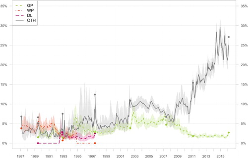
Among the smaller parties, we see a relatively modest presence of the Worker's Party and Democratic Left in the 1980s and 1990s (see Figure 2). The Green Party is regularly included in polls from 1989 and shows a varying level of success: almost always under 5 per cent during the 1990s, while in the 2002–2007 term support raised just above that level. The party lost most of that support again, however, over the course of the 2007 parliament, when it participated in a coalition government with Fianna Fáil and the Progressive Democrats. Since 2011, the Green Party has been a very stable party at about 2 per cent. A remarkable development is visible for the category of ‘others’, which includes both minor parties and independent candidates. This category was relatively unimportant in the 1990s, generally polling under 5 per cent, although support often peaked around elections and also seems to be underestimated somewhat in the polls. In the 2000s, however, and particularly in the 2010s, support for this group of parties and independents is rising very quickly to a point where together they formed the largest group in the polls. Indeed, independent candidates and new parties did very well in the 2016 elections.

Figure 1. Support for Fianna Fáil, Fine Gael, Labour, Sinn Féin and the Progressive Democrats 1987–2016. Note: Mean estimates and 95% credible intervals (shaded). The dots represent election results.

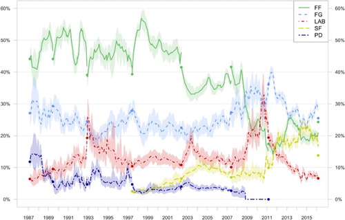
Figure 2. Support for the Green Party, Worker's Party, Democratic Left and Others 1987–2016. Note: Mean estimates and 95% credible intervals (shaded). The dots represent election results. For the ‘Others’ category, the parties included in it vary from election to election.

Party support is more variable during some terms than others. Take, for example, the Labour party: we see large volatility in support between 1992 and 1997, with relatively large credible intervals. In the subsequent term, Labour's support was much more stable, which results in more certainty in our estimates. For most parties, the estimated intervals shrink considerably over time, in particular in the last period. The reason is quite simple: the volume of polls increases a lot over time, with 46 polls included in the analysis for 1992–1997, compared to 64 polls between 2007–2011 and 148 in the 2011–2016 parliamentary term. Taking into account differences in length, the number of polls per year increases from just over 7 in the first period included, to almost 30 in the most recent term. Prior to 2011, there would be considerable periods of time without any polls being published, which results in a relatively large credibility interval for those time periods. This is entirely correct, as we cannot be too certain about the development of party preferences during those times.

Even though the aggregation model proposed in this paper is not intended as a forecast model, observers might be interested to see in the differences between final estimates and general election outcomes. After all, if an aggregate of polls would bear no resemblance at all with the final outcome, perhaps we should advice voters and parties not to pay much attention to them. Figure 3 displays the Polling Indicator estimate on the day before a general election (in black) and the outcome of that election in grey. In a large majority of cases, the election result falls within the credible intervals of the model's estimates. There are, however, a number of cases where this is not true. In particular, there seem to be differences between Fianna Fáil's poll scores and their general election results. For the general elections in 1989, 1992, 1997 and 2002, the party consistently scored higher in the polls than in the general elections (the difference is significant in 1989 and 2002 but not in the other years). In the early 2000s, polling companies started to ‘adjust’ their figures for this Fianna Fáil over-representation, which actually resulted in an aggregate measure that seems to have underestimated Fianna Fáil support in the 2007, 2011 and 2016 elections (although in 2010 Ipsos MRBI had already ceased their use of adjustments). For other parties, there are also occasional significant differences between the final poll and the election result, but this occurs in only one or two elections per party. Still, we do observe that generally both Fine Gael and Independents/Others seem to do somewhat better on polling day than the average final poll would suggest, at least up to 2007. These differences were not statistically significant in most cases, but the stability of the pattern across elections seems to suggest that the reverse side of the Fianna Fáil over-representation in the polls as a (small) under-representation of Fine Gael and Others.

Figure 3. A comparison between final Polling Indicator estimates and General Election results.

Overall, the mean squared error of the difference between the percentages obtained in the final Polling Indicator and the General Election result varied from 5.65 in the 2016 election, to only 0.97 in the 2011 election.¹⁰ The 2016 election suffered from an under-estimation of Fianna Fáil while Fine Gael was overestimated. In addition, in the 2016 elections the poll aggregation included fewer smaller parties, which generally show a smaller error and therefore keep down the mean squared error .¹¹ In earlier years, such as the poor showing at the 2002 election the error was usually focused on only one party (Fianna Fáil). Marsh and McElroy (2003) analyze the 2002 case in detail and find that sampling bias is likely the main source of error, after discarding alternative explanations (late swing, differential turnout and dealing with undecideds). In the remaining years the mean squared error was between 2 and 4. While this does imply that predictions from the polls do contain error and likely also bias for certain parties, overall the aggregation of polls does give a fair indication of how parties will do on election day. On average, the aggregate of polls deviated from the election result by between, on average, 0.73 per cent (2011) and 1.99 per cent per party (2016). In most cases that is clearly better than the poorest poll and quite close (or even better than) to the best poll.

4.1. Systematic and random error

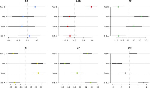
The aggregation model takes into account that there are systematic differences between pollsters, so-called house effects. The house effects reported here are to be interpreted as relative to the average pollster. In order to identify the model, house effects are assumed to sum to zero. In this sense, the aggregation provides an average of the polls. Basically, pollsters are estimated to consistently over- or underestimate party support for a certain party compared to other pollsters. For example, in the 2011–2016 term, Red C Research put Labour consistently higher by just shy of a percentage point, compared to the average pollster (see Figure 4). This might be explained by the fact that Red C weights its polls halfway between voting intention and previous voting behaviour. As Labour did much better in the 2011 election than most of the polls between 2011 and 2016, weighting in previous voting behaviour is likely to increase Labour support. Figure 4 concerns the most recent completed term, which is most interesting as four different pollsters were active during this period. There was no significant house effect for Fine Gael polls, but there was for the other parties. For Fianna Fáil, Behaviour & Attitudes is generally on the lower side, while Millward Brown was most optimistic about this party's fortunes. There are reasonably large house effects for Sinn Féin, with both Red C and B&A showing negative house effects of and Millward Brown and Ipsos MRBI display positive house effects of . This means that the average polls for these pollsters differ by over 2 percentage points. There were also considerable house effects for ‘others’, where Millward Brown was about 2.5 per cent more negative about their support than Behaviour & Attitudes. While these effects may not be groundbreaking, they are significant and substantially relevant.

Figure 4. House effects in the Irish Polling Indicator (2011–2016). Note: dots display house effect for each pollster (95% credible intervals in black). , , , .

Apart from the systematic differences between pollsters, the aggregation model also takes into account that the random error associated with poll estimates may be larger (or smaller) than under random sampling. In all but one of the terms studied, this ‘design effect’ or ‘pollster-induced random error’ factor was indeed larger than one, suggesting that polling estimates were more variable than to be expected under random sampling (see Figure 5). This is not unexpected as many pollsters use a limited number of sampling points for their face-to-face interviews. As a result, there is an element of clustering in the sample, which should increase the standard error somewhat. It is, however, difficult to be entirely sure of the size of this effect. First of all, low polling volumes make it difficult to estimate this effect very precisely, with the prior distribution on parameter D affecting the estimates. In the most recent term, however, poll estimates were also be found to show more variability than is to be expected under random sampling, while for this period we do have a relatively large sample of polls (and the prior distribution has much less effect on the findings). Therefore, we can be reasonably sure that pollster-induced error does play a role in the Irish case with error margins likely to be somewhat underestimated by the simple formulas used for the case of random sampling.

Figure 5. Design effects. Note: values indicate how many times larger the confidence intervals of individual poll estimates were estimated to be, compared to random sampling. A value of 1 would mean that the random error associated with the polls would be exactly the same as under random sampling. Larger values indicate that more error is associated with the poll estimates (error bars represent 95% credible intervals).

5. Incorporating shocks into poll aggregation models

Poll aggregation models are good at distilling trends from (noisy) polling data. When one new poll with remarkable outcomes is published, one's response should be ‘it is only one poll’, and that is exactly how aggregation models treat these polls. Information from the new poll is compared to previous polls. If the new poll is somewhat higher than the polling average, even correcting for house effects, it is much more likely to be just noise than represent a ‘real’ trend. Thus, polling aggregation models dampen outliers and are generally somewhat conservative about ‘breaking polls’.

While this is generally a good approach, in certain situations it might lead the aggregation models to underestimate change. If a party drops five percentage points in the polls after a major corruption scandal, that is much more likely to represent a true effect than if the same change happens after the party was not in the news at all. In other words, if there is prior information about important political events that should affect our beliefs as to whether drops or increases in party polls represent true effects.

The random walk model used in the model above allows party support to change more on some days than on others. Still, change is estimated to be relatively small from day to day. This is true for most days, but there are major political events that seem to ‘break through the random walk’. Mid-term elections and important societal events, such as the Bank Guarantee in Ireland in 2008, are examples. After such events, party support might change dramatically overnight. Such change might be so extreme that the random walk parameter does not represent it very well.

The proposed solution here is to modify the random walk model, by multiplying by a factor :(8)

where s represents the instance of shock, with s=1 representing the normal random walk and representing days with major political events:(9) (10)

Effectively, this means that on ‘shock days’ support for a party is allowed to make a much bigger step in the random walk than on normal days. As is estimated in the model, it is not necessary that there will be a large change in party support on those ‘shock days’: if polls before and after the ‘shock day’ are stable, will be estimated to be (close to) unity. If there is a large change in polls, however, the parameter makes it much more likely that this is interpreted as real change rather than a large outlier in the polls. This is reasonable, because our knowledge about relevant political circumstances indeed tells us that changes in party support around the time of the ‘shock day’ are likely to be real.

5.1. Ireland 2008–2010

The financial and economic crisis has dominated Irish politics since the 2007 elections. In particular in the 2007–2011 term, there were large changes in voters' party preferences. Fianna Fáil lost its long-time-dominant position and ended up as the third party at the 2011 election. The economic and financial crisis presented a number of shocks, both to the economy as well as to public opinion. Marsh and Mikhaylov (2012) identify two important moments in particular: the introduction of the bank bailout on 30 September 2008 and the Withdrawal from the bond market by the Irish state on 30 September 2010. These shocks arguably affect public opinion regarding the main government party of the day, Fianna Fáil.

The Irish Polling Indicator does not, however, show particularly large changes in public opinion around those dates. The green line in Figure 6 shows that while there was a decline in support around those two pivotal moment in the economic crisis, the timing was off. If we look at individual polls, however, we do see a large decline before and after the Bank Guarantee (from 36 per cent to 26 per cent in the Red C Research polls). The aggregation model, however, seems to smooth out this decline over a longer period of time, implicitly assuming that the September polls might just be a little on the high side and the October polls a bit on the low side. Something similar is visible in 2010, when the Fianna Fáil declines, but only from the end of October.

Figure 6. Support for Fianna Fáil 2008–2010. Note: Dots represent individual polls, colour coded: , , . Credible intervals have been omitted from the figure for reasons of clarity.

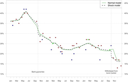
When the model is rerun with the ‘shock’ specification outlined above, the shocks to party support appear to be larger than in the original model. Support for Fianna Fáil is estimated to remain at about 34 per cent before the Bank Guarantee was announced, to drop to just under 30 per cent the day after. Similarly, at the end of September 2010 party support drops by about 3.5 per cent after Ireland withdraws from the bond markets. In both cases, the decline is not quite as pronounced as individual polls seem to suggest. In 2008, this is reflective of the fact that later polls gave somewhat higher estimates for Fianna Fáil than the 26 per cent low in October 2008. In 2010, party support was not quite as high in the Polling Indicator (21.5per cent) compared to an Ipsos poll just taken before the withdrawal (24 per cent).

The modification suggested above seems to be able to capture sudden changes in party fortunes better than the normal specification. The good news for polling aggregation methods is that after some time, both the ‘normal’ and ‘shock’ measures converge. Still, if one is interested in the impact of one specific important political event on party support, the ‘shock’ modification seems appropriate as not to underestimate changes in public opinion in the short term.

We can further analyze the effect of the two major economic events on Fianna Fáil support by replicating the analysis in Marsh and Mikhaylov (2012). Using polling data from Red C Research, they estimated a simple regression model in which support for Fianna Fáil was modelled as a function of five variables. Two of the five were dummy variables: Bank Guarantee (0 before the Bank Guarantee, 1 afterwards) and Withdrawal from the bond market (0 before, 1 after). Three others were continuous time variables. Time starts at 0 at the month of the election in 2007 and increases by 1 every month. ‘After Bank Guarantee’ is 0 before the Bank Guarantee and then increases by 1 every month afterwards. Similarly, ‘After withdrawal from bond market’ is coded 0 before that 2010 event and increasing after. The simple model used by Marsh and Mikhaylov (2012) is well-equipped to explain variation in Fianna Fáil support (see Table 1). The adjusted for their model is 0.83 with a root mean squared error of 3.3. They find a strong effect of both the Bank Guarantee and Withdrawal from the bond market on Fianna Fáil support.

Table 1. Explaining support for Fianna Fáil 2005–2011.

	Model 1 (MM)	Model 2 (TL)
(Intercept)
Time	0.08
Bank Guarantee
After Bank Guarantee
Withdrawal from bond market
After withdrawal from bond market	0.07
Adj.	0.83	0.96
Num. obs.	66	1999
RMSE	3.3	1.54

Note: Model 1 has been reproduced from Marsh and Mikhaylov (2012: 481). . . .

I replicated the analysis using the ‘shock model’ time series presented above.¹² Because this model presents an estimate of party support for each day, rather than using each month as a case, I used daily data. To allow for an easy comparison between the models, my time variables are expressed in (fractions of) months as well.

The main findings are very similar between models (see Table 1). I find a large impact of the Bank Guarantee on Fianna Fáil support in the slightly longer run. Although the immediate effect of the Bank Guarantee was estimated to be just over 4 per cent, levels of support for Fianna Fáil declined further to a much lower level after the Bank Guarantee. This effect is estimated to be almost 12 percentage points. The Withdrawal from the bond market also affected Fianna Fáil support negatively, by about 3.7 percentage points, according to Model 2. Moreover, I find negative time trends after the major economic events. The model fit for this daily time series is very good (), which is even higher than the Marsh and Mikhaylov model.¹³ One explanation might be that the aggregation model presents less ‘noisy’ indicators of party support in polls than individual polls do; therefore, it would be easier to explain the variance in that support using structural explanations.¹⁴

6. Discussion: using poll aggregation to improve media reports of opinion polls

The results show that both random error and systematic differences between pollsters should be taken into account when interpreting opinion poll results. This is exactly where poll aggregation can be used to improve media coverage of opinion polls. The first lesson to be taken from this would be that reports on opinion polls should take account of all available polls, not just those from one company that did the most recent poll. The Irish Polling Indicator makes house effects, systematic differences between pollsters, explicit. Part of the explanation why a party might do particularly well in a poll might be that it always does better in polls by that pollster. Even when media outlets report in detail about a specific poll commissioned by them, they should not prove blind and deaf to the information contained in other polls. They help to interpret the results: is this increase for a party likely to represent true change, or might it just be random noise? It would of course be even better to report the results of poll aggregation models alongside with individual polls. This puts the individual poll into context and shows that random and systematic error should be taken into account.

The second lesson is to take account of uncertainty associated with polls. While most academics are at ease when dealing with uncertainty, it sometimes seems to irk journalists and the general public. This all too often leads to one of two responses: either to forget about uncertainty altogether and interpret all changes in polling support as real or to argue that polls tell us absolutely nothing because of all that uncertainty involved. This black and white view of opinion polls does not do justice to their usefulness. While Irish media do quite often include basic relevant information about opinion polls, such as when the poll was taken, the number of respondents and the associated margin of error, sometimes the description of the results does not take account of the disclaimer. Regularly, small differences between parties and small changes in parties' fortunes are interpreted as ‘true’, while these are quite likely to represent random error (‘noise’). Many media could do a better job at reporting uncertainty margins associated with polls. Data from the Irish Polling Indicator is very suitable for this aim. The Bayesian specification of the models allows for an intuitive understanding of the uncertainty (credibility intervals) associated with the estimates. It is easy and correct to report that ‘according to the Irish Polling Indicator, we are 95% certain that support for Fine Gael lies between 25 and 29 %'.¹⁵ Moreover, it is possible to directly estimate the probability that a party saw its support increase or decrease compared to one week or month ago, as the Polling Indicator produces draws from the posterior distribution of the variables of interest. Similarly, we can calculate from the posterior distribution whether one party is larger or smaller than another one.

The third lesson would be to use polls for what they are good at: describing and explaining trends. As far as describing the trend goes, polling aggregation provides richer data than individual pollsters can, because it takes into account all available data. When it comes to explaining (changes in) party support, however, specific polls have much to add. They can provide insight in which voters change their party preference: where do they come from, what is their background and what are their views? Reports of individual polls should, more than is the case now, focus on this added value. This way polling aggregation and results from individual polls can be combined to provide better insights into voters' preferences.

7. Conclusion

This article presented a poll aggregation method for Irish election that has the potential to inform voters better about parties' political fortunes. It tackles the challenge of aggregating opinion polls in a multi-party setting with a limited number of polls outside election time, especially before 2007. This contribution is particularly relevant for voters and political actors in Ireland, who may use the results to gain a better understanding about strengths and limitations of opinion polls. In comparative terms, the model presented here combines various insights in opinion poll aggregation. It moves beyond the two-party case by modelling support for all parties together, ensuring that support sums to 100 per cent (Hanretty et al., 2016). At the same time, it incorporates house effects as well as an estimate of design effects, which makes explicit that random polling error is usually larger in the Irish case than under simple random sampling (Fisher et al., 2011). Finally, it presents a way to incorporate shocks to the political system into the model. This makes poll aggregation more useful in cases where we want to estimate the effect of an event on party support. Further work is, however, necessary to explore the consequences of the proposed ‘shock’ adjustment in other settings.

Work on the Irish case could be extended in multiple directions. First, one could use these estimates as a starting point for estimating the number of seats each party stands to win (Fisher et al., 2011; Hanretty et al., 2016). Because of the complications of the Single Transferable Vote system in small multi-member constituencies and the importance of vote transfers, this would require additional data and modelling regarding the geographical distribution of party support as well as transfer patterns between parties. Second, one could move from an aggregation model of opinion polls to a forecast model of elections. To do this, one needs to take into account historical patterns of polling bias, as well as the additional error involved in projecting current polls onto election results in the future. Work on this in the United States and the United Kingdom has achieved a high level of sophistication, which could be used to pursue a similar enterprise in Ireland. While election forecasting per se should perhaps not be a primary aim of academic political science research, these studies help us to understand biases and uncertainty in polling better and thereby help to contribute to a better understanding of opinion polls by parties, journalists and hopefully the general public.

Acknowledgments

An earlier draft of this paper has been presented at the Annual Conference of the Political Studies Association of Ireland (PSAI), Cork, 16–18 October 2015. I am thankful for the research assistance in collecting the polling data that has been provided by David Beatty and Stefan Müller. I thank Stefan Müller for his comments on an earlier draft of this paper.

Disclosure statement

No potential conflict of interest was reported by the author.

ORCiD

T. Louwerse http://orcid.org/0000-0003-4131-2724

Additional information

Funding

This paper makes use of data collected for the project ‘Between mandate and responsiveness: how electoral uncertainty affects political representation’, which is supported by Arts and Social Sciences Benefactions Fund (Trinity College, Dublin).

Notes

1 Pollster Red C makes use of Random Digit Dialling with a 50–50 split between mobile phones and landlines.

2 Ideally, this parameter would be allowed to vary between pollsters. In practice, however, if this is allowed, the model tends to estimate a tiny design effect for the most popular pollster, resulting in an estimate that very closely follows the polls of that particular pollster. Pickup et al. (2011) report similar issues. Therefore, I estimate a single industry-level design effect.

3 In the mathematical notation, I will specify the variance of the normal distributions. The JAGS script in the appendix uses the precision, which is the inverse variance.

4 As Ipsos MRBI changed its adjustment method during the 1997–2002 and the 2007–2010 term, we split these terms into multiple parts (three and two, respectively) (Marsh and McElroy, 2003: 163). For each part, we estimate the house effects separately (each subject to the zero-sum constraint discussed below).

5 Moreover, the implementation of the model is more difficult as the software used to estimate this model, JAGS, does not allow for missing values in the vector of counts.

6 I also experimented with non-logged ratios, but this requires the implementation of a truncated normal distribution in the random walk model, which means that the algorithm runs less quickly. The results, however, were rather similar to the log-ratio approach.

7 An alternative approach is to set to the prior election result and assume that differences between that election and subsequent polls are due to house effects (Fisher et al., 2011). This strategy has the advantage that it allows us to correct for ‘industry bias’, that is under- or overestimation of a party by all pollsters. The problem is, however, that relatively few polls are done after an election. In the Irish case this is particularly true, with sometimes a few months passing between elections and the first post-electoral poll. One solution would be to fix the parameter , where n is the last day observed, to the subsequent election result (Jackman, 2005). This option is, of course, only feasible for historical data, not the current term. Moreover, one has to assume that the day-to-day change is similar in the final stages of the election campaign compared to the entire period; this assumption might not necessarily hold.

8 Strictly speaking, the house effect prior is over the unstandardized house effect. Also note that the prior for the variance of the random walk is over rather than .

9 If a party's support was not included in the breakdown of only a few polls, for these polls the party support (as well as support for ‘others’) was defined as missing. One advantage of the aggregation model above, estimated using Markov Chain Monte Carlo methods is that it allows for flexibility regarding missing values.

10 Omitting parties that did not participate in these elections, but were polled on in the previous term (WP 1992–1997 and PD 2007–2011).

11 If we limit the MSE to the three traditional large parties in Irish politics, the mean squared error was highest in 2002 (8.19), just before 2016 (7.12) and 2007 (6.98). The lowest mean squared errors for those three parties occurred in 2011 (1.52).

12 The analysis of Marsh and Mikhaylov starts in September 2005; therefore, for the period between September 2005 and 2007 I use the estimates from the regular polling indicator for that time period.

13 This is also true () when we limit the model to one observation per month resulting in 66 monthly observations.

14 I also replicated the Marsh & Mikhaylov model using the original Irish Polling Indicator series. Findings are similar except for Withdrawal from the bond market, which loses significance. This seems to support the case for taking into account major events when modelling opinion polls.

15 Note that confidence intervals associated with frequentist statistics, such as error margins associated with individual opinion polls, cannot generally be interpreted this way. Frequentist 95 per cent confidence intervals should contain the population mean in 95 per cent of times across an infinite number of replications.

Appendix. JAGS code for model estimation

The models presented here are are based on those presented by Jackman (2005) and Hanretty et al. (2016), using parts of their JAGS/BUGS code.

A.1. Main model

model{

#Equation 1: Define reported poll percentage as sum of true percentage

# and house effect

for(k in 1:NPARTIES) {

 for(i in poll_start [k]:poll_end  [k]){

 mu [i,k] <- alpha [date [i],k]+house [org [i],k,houseperiods [i]]

 y [i,k]∼ dnorm(mu [i,k],prec [i,k])

 prec [i,k] <- 1 / (vari [i,k] * pie)

 }

}

# Equation 2: Random walk model

# For party 1, we have specified alphalog = 0 in data

for(k in 2:NPARTIES) {

 alphalog [period_start [k] - 1, k]∼ dunif(logstart_min [k],logstart_max [k])

 for(i in period_start [k]:period_end [k]){

  alphalog [i,k]∼ dnorm(alphalog [i-1,k],tau [k])

 }

}

# Equation 3: Derive alphas from alphalog

for(i in 1:NPERIODS){

 for(k in 1:NPARTIES) {

  alphaexp [i,k] <- exp(alphalog [i,k])

  alpha [i,k] <- alphaexp [i,k] / sum(alphaexp [i,])

 }

}

# Equation 4: Prior over random walk

for(k in 1:NPARTIES) {

 tau [k] <- pow(sigma [k], -2)

 sigma [k]∼ dunif(0,.2)

}

# Equation 5: Prior over house effect + sum-to-zero constraint

for(j in 1:NHOUSEPERIODS) {

 for(i in 1:NHOUSE){

  for(k in 1:NPARTIES) {

   house_us [i,k,j]∼ dunif(-.2,.2)

   house [i,k,j] <- house_us [i,k,j] - inprod(house_us [,k,j],
houseweights [,j])

  }

 }

}

# Equation 6: Prior over pollster induced error

pie ∼ dunif(1/3, 3)

}

A.2. Shocks model

model{

# Equation 1: Define reported poll percentage as sum of true percentage

# and house effect

for(k in 1:NPARTIES) {

 for(i in poll_start [k]:poll_end [k]){

  mu [i,k]<- alpha [date [i],k]+ house [org [i],k,houseperiods [i]]

y [i,k]∼ dnorm(mu [i,k],prec [i,k])

prec [i,k] <- 1 / (vari [i,k] * pie)

 }

}

# Equation 7: Random walk model

# For party 1, we have specified alphalog = 0 in data

for(k in 2:NPARTIES) {

 alphalog[period_start [k]- 1, k]∼ dunif(logstart_min [k],logstart_max[k])

 for(i in period_start [k]:period_end [k]){

  alphalog  [i,k]∼ dnorm(alphalog [i-1,k],tau [k] * shocksize [shocknumber [i]])

 }

}

# Equation 3: Derive alphas from alphalog

for(i in 1:NPERIODS){

for(k in 1:NPARTIES) {

 alphaexp [i,k] <- exp(alphalog [i,k])

  alpha [i,k] <- alphaexp [i,k] / sum(alphaexp [i,])

 }

}

# Equation 4: Prior over random walk

for(k in 1:NPARTIES) {

 tau [k] <- pow(sigma [k], -2)

 sigma [k] ∼ dunif(0,.2)

}

# Equation 5: Prior over house effect + sum-to-zero constraint

for(j in 1:NHOUSEPERIODS) {

 for(i in 1:NHOUSE){

  for(k in 1:NPARTIES) {

   house_us [i,k,j] ∼ dunif(-.2,.2)

   house [i,k,j] <- house_us [i,k,j] - inprod(house_us [,k,j],
houseweights [,j])

  }

 }

}

# Equation 6: Prior over pollster induced error

pie ∼ dunif(1/3, 3)

# Equation 8,9: Define priors for shocks

shocksize [1] <- 1

for(i in 2:NSHOCKS) {

 shocksize [i] ∼ dunif(0.0001,1)

}

}

References

- Arceneaux, K. & Nickerson, D.W. (2009) Modeling certainty with clustered data: a comparison of methods, Political Analysis, 17(2), pp. 177–190. doi: 10.1093/pan/mpp004
- Brüggen, E., Van den Brakel, J. & Krosnick, J. (2016) Establishing the Accuracy of Online Panels for Survey, CBS Discussion Paper, No. 4, available at: https://www.cbs.nl/en-gb/background/2016/15/establishing-the-accuracy-of-online-panels-for-survey-research (accessed 16 May 2016).
- Cantu, F., Hoyo, V. & Morales, M.A. (2015) The utility of unpacking survey bias in multiparty elections: Mexican polling firms in the 2006 and 2012 presidential elections, International Journal of Public Opinion Research, available at: http://ijpor.oxfordjournals.org/cgi/doi/10.1093/ijpor/edv004.
- Crespi, I. (1988) Pre-Election Polling: Sources of Accuracy and Error (New York: Russell Sage Foundation).
- Fisher, S.D., Ford, R., Jennings, W., Pickup, M. & Wlezien, C. (2011) From polls to votes to seats: forecasting the 2010 British general election, Electoral Studies, 30(2), pp. 250–257. doi: 10.1016/j.electstud.2010.09.005
- Hanretty, C., Lauderdale, B. & Vivyan, N. (2016) Combining national and constituency polling for forecasting, Electoral Studies, 41(March), pp. 239–243. doi: 10.1016/j.electstud.2015.11.019
- Hobolt, S.B. & Klemmensen, R. (2008) Government responsiveness and political competition in comparative perspective, Comparative Political Studies, 41(3), pp. 309–337. doi: 10.1177/0010414006297169
- ISSDA. (2015) Opinion Poll Data, available at: https://www.ucd.ie/issda/data/opinionpolldata/.
- Jackman, S. (2005) Pooling the polls over an election campaign, Australian Journal of Political Science, 40(4), pp. 499–517. doi: 10.1080/10361140500302472
- King, G., Keohane, R.O. & Verba, S. (1994) Designing Social Inquiry: Scientific Inference in Qualitative Research (Princeton: Princeton University Press).
- Kish, L. (1957) Confidence intervals for clustered samples, American Sociological Review, 22(2), p. 154. doi: 10.2307/2088852
- Lago, I., Guinjoan, M. & Bermúdez, S. (2015) Regulating disinformation, Public Opinion Quarterly, available at: http://poq.oxfordjournals.org/lookup/doi/10.1093/poq/nfv036.
- Marsh, M. (2006) Irish Opinion Poll Archive, available at: http://www.tcd.ie/Political_Science/IOPA/.
- Marsh, M. & McElroy, G. (2003) Why the opinion polls got it wrong in 2002, in: M. Gallagher, M. Marsh & P. Mitchell (Eds.) How Ireland Voted 2002, pp. 159–159 (Basingstoke: Palgrave Macmillan).
- Marsh, M. & Mikhaylov, S. (2012) Economic voting in a crisis: the Irish election of 2011, Electoral Studies, 31(3), pp. 478–484. doi: 10.1016/j.electstud.2012.02.010
- McElroy, G. & Marsh, M. (2008) The polls: a clear improvement, in: M. Gallagher & M. Marsh (Ed.) How Ireland Voted 2007, pp. 132–132 (Basingstoke: Palgrave Macmillan).
- Mellon, J. & Prosser, C. (2015) Why Did the Polls Go Wrong?, available at: http://www.britishelectionstudy.com/bes-resources/why-did-the-polls-go-wrong-by-jon-mellon-and-chris-prosser/.
- Pickup, M. & Hobolt, S.B. (2015) The conditionality of the trade-off between government responsiveness and effectiveness: the impact of minority status and polls in the Canadian house of commons, Electoral Studies, available at: http://linkinghub.elsevier.com/retrieve/pii/S0261379415001444.
- Pickup, M., Scott Matthews, J., Jennings, W., Ford, R. & Fisher, S.D. (2011) Why did the polls overestimate liberal democrat support? Sources of polling error in the 2010 British general election, Journal of Elections, Public Opinion & Parties, 21(2), pp. 179–209. doi: 10.1080/17457289.2011.563309
- Plümmer, M. (2013) JAGS: Just Another Gibbs Sampler, available at: http://mcmc-jags.sourceforge.net/.
- Silver, N. (2012) The Signal and the Noise: The Art and Science of Prediction (London: Allen Lane).
- Soroka, S.N. & Wlezien, C. (2010) Degrees of Democracy Politics, Public Opinion, and Policy (New York: Cambridge University Press).
- Squire, P. (1988) Why the 1936 literary digest poll failed, Public Opinion Quarterly, 52(1), p. 125. doi: 10.1086/269085
- van der Meer, T.W.G., Hakhverdian, A. & Aaldering, L. (2015) Off the fence, onto the bandwagon? A large-scale survey experiment on effect of real-life poll outcomes on subsequent vote intentions, International Journal of Public Opinion Research, 51(4), pp. 769–784.
- Walther, D. (2015) Picking the winner(s): forecasting elections in multiparty systems, Electoral Studies, 40, pp. 1–13. doi: 10.1016/j.electstud.2015.06.003