Continuous cuffless and non-invasive measurement of arterial blood pressure—concepts and future perspectives

Abstract

Hypertension diagnosis is one of the most common and important procedures in everyday clinical practice. Its applicability depends on correct and comparable measurements. Cuff-based measurement paradigms have dominated ambulatory blood pressure (BP) measurements for multiple decades. Cuffless and non-invasive methods may offer various advantages, such as a continuous and undisturbing measurement character. This review presents a conceptual overview of recent advances in the field of cuffless measurement paradigms and possible future developments which would enable cuffless beat–to–beat BP estimation paradigms to become clinically viable. It was refrained from a direct comparison between most studies and focussed on a conceptual merger of the ideas and conclusions presented in landmark scientific literature. There are two main approaches to cuffless beat–to–beat BP estimation represented in the scientific literature: First, models based on the physiological understanding of the cardiovascular system, mostly reliant on the pulse wave velocity combined with additional parameters. Second, models based on Deep Learning techniques, which have already shown great performance in various other medical fields. This review wants to present the advantages and limitations of each approach. Following this, the conceptional idea of unifying the benefits of physiological understanding and Deep Learning techniques for beat–to–beat BP estimation is presented. This could lead to a generalised and uniform solution for cuffless beat–to–beat BP estimations. This would not only make them an attractive clinical complement or even alternative to conventional cuff-based measurement paradigms but would substantially change how we think about BP as a fundamental marker of cardiovascular medicine.

PLAIN LANGUAGE SUMMARY

• This concept review wants to highlight the current state of non-invasive cuffless continuous blood pressure estimation.

• Cuffless blood pressure measurement devices usually rely on pulse wave velocity.

• Pulse wave velocity is mostly calculated via measuring pulse arrival time.

• Using pulse transit time instead of pulse arrival time showed improved results.

• Additional biomarkers like heart rate, photoplethysmogram intensity ratio or heart rate power spectrum ratio can be used to improve measurement precision.

• For cuffless and cuff-based devices intended for 24-hour BP measurements, a more refined validation protocol is required.

• The ESH assesses the measurement accuracy of cuffless devices as unclear and does not recommend hypertension diagnosis based on cuffless devices.

• Machine Learning and Deep Learning applications are a powerful tool to generate complex algorithms, which can be used to estimate blood pressure.

• Selecting biomarkers like pulse wave velocity, heart rate, etc. as input features for Deep Learning systems would be a very promising approach to measure blood pressure more precise.

Keywords:

• Blood pressure measurement
• pulse wave velocity
• deep learning
• hypertension
• pulse transit time

Introduction

The monitoring of blood pressure (BP) and the proper treatment of arterial hypertension are one of the central building blocks of modern medicine. Today, around 30%−45% of the adult European population suffers from arterial hypertension [1]. BP measurements are widely reliant on cuff-based measurement devices. As research has shown the improved diagnostic value of out-of-office ambulatory BP measurements (ABPM) over standard in-office measurements, medical attention has shifted towards 24-h measurement paradigms [1,2]. Cuff-based BP measurements pose some major drawbacks: Cuff inflations come with patient discomfort, which is deemed to especially affect nocturnal BP levels due to sleep arousal [3–5]. As nocturnal BP values show the highest predictive value for a range of cardiovascular diseases and overall cardiovascular death, this side-effect of nightly cuff-inflations is a challenge for cardiovascular diagnostics [6–9]. Due to these disadvantages of the cuff, there are attempts to reduce the duration and frequency of cuff-based measurements while maintaining diagnostic power [10].

Further, increased BP variability has been linked to increased all-cause mortality, strokes, and coronary heart disease [11,12]. The most promising approach for interpreting BP variability is through continuous measurements, as they allow for more precise and refined variance analyses.

In the wake of enabling non-invasive cuffless BP estimation designs, two main approaches have solidified themselves: Hand-crafted models, based on physiological understanding and Machine Learning models, taking advantage of the recently discovered power of Deep Learning architectures.

Cuffless BP measurement paradigms seem suited to mitigate the drawbacks of cuff-based measurement devices while allowing for continuous, beat–to–beat measurements. Although the approach of cuffless BP measurement has great potential, the evaluation of and comparison between these devices still shows difficulties. A suitable validation method has not yet been established. The European Society of Hypertension (ESH) describes the validation of cuffless devices using the ESH’s International Protocol for short term scenarios to be of limited use. Therefore, the ESH assessed the measurement accuracy of cuffless BP measurement devices as unclear. Subsequently, the ESH does not recommend hypertension diagnosis based on cuffless devices. Further methodological and clinical evidence in the field is demanded [13,14].

This concept review wants to highlight the current state of non-invasive cuffless BP estimation and promising future developments, which can promote cuffless BP estimation given the recommended evidence, can be provided in the future. For explanatory reasons, the two paradigms of physiological and Deep Learning based BP estimation are first introduced separately. Following this, a new conceptual approach of unifying the advantages of each of the two paradigms into a single paradigm is presented. To achieve this, this review focusses only on recent landmark literature describing new conceptual developments in cuffless BP estimation and does not aim to provide an overview over all related scientific literature. Ultimately, this review wants to propose multiple possible options to uplift cuffless BP estimation into clinical viability.

Pulse wave velocity (PWV)

This part presents the basic concepts of physiological models for cuffless BP measurement and their limitations. Introductory information is concisely presented at the beginning of each paragraph. Technical details about the underlying formula are presented at the end of each paragraph and may be taken as an additional mathematical illustration for interested readers.

BP estimation via PWV

In 1984, Callaghan et al. have shown the applicability of the Moens-Korteweg-equation for canine arteries, which describes the dependency of the PWV on BP differences [15]. This equation has been interpreted for human BP levels and subsequently successfully applied for experimental BP estimation. To achieve this, a surrogate marker for PWV had to be found. Modern physiological cuffless BP estimations predominantly rely on PWV surrogates. Generally, the pulse arrival time (PAT) presented itself suitable, as for its comparably easy detection, as well as its direct connection to the PWV [16].

PAT as a surrogate marker for PWV

PAT is defined by the time difference between heart excitation and the arrival of the peripheral pulse wave. In practice, this can be measured by detecting the time difference between an electrocardiogram (ECG) Q- or R-wave and the arrival of the peripheral pulse wave, seen in a pulse-plethysmography (PPG; Figure 1 and Table 1) [16–18]. (1) $$c\mathrm{ }=\mathrm{ }\sqrt{\frac{1}{p}\mathrm{ }·\mathrm{ }\frac{dP}{dV}\mathrm{ }·\mathrm{ }V}$$(1) (2) $$\mathrm{PWV}=\mathrm{ }\frac{l}{\mathrm{PAT}}$$(2) where c = PWV = pulse wave velocity, p = blood density, dP = inner vessel pressure difference, dV = inner vessel volume difference, V = inner vessel volume, l = total vessel length of blood flow, and PAT = pulse arrival time (Figure 1).

Figure 1. Left panel: Technical design for PAT measurement: ECG for detection of the Q- or R-wave, PPG for detection of the peripheral volume pulse. Recorder: data collection, AD-conversion, data pre-processing, storage. Right panel: PAT-Detection from ECG and PPG, here from the start of Q-wave to the beginning of PPG signal rise. In the literature, several other points in the physiological signals, such as the R-wave peak or the steepest increase of the PPG signal have been used for PAT detection. This results in different PAT values.

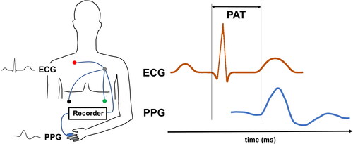
Table 1. Recent studies focussing on improving cuffless BP measurements.

Authors	Year	Suggested metrics	Measurement devices	Validation measurement devices	Δ Mean ± SD Validation	Ref.
Results in 24-hour ABPM measurement
Socrates et al.	2021	PAT	ECG PPG (finger)	osc. sphygmomanometer	SBP: 5.1 ± 6.2 DBP:4.2 ± 4.4	[38]
Results in laboratory setting
Beutel et al.	2021	PAT	ECG PPG (finger)	Finapres osc. sphygmomanometer	SBP: 4.2 ± N/A DBP: 4.8 ± N/A	[22]
Block et al.	2020	PAT	ECG PPG (ear, finger, toe)	auscultatory sphygmomanometer	SBP: N/A DBP: N/A	[20]
Moharram et al.	2020	PAT	ECG PPG (finger)	invasive measurement osc. sphygmomanometer	SBP: 34.3 ± N/A DBP: 23.6 ± N/A	[39]*
Yousefian et al.	2019	PTT	ECG BCG PPG (wrist)	Finapres	SBP: 7.6 ± N/A DBP: 5.1 ±N/A	[23]
Chen et al.	2018	PAT + PIR + HPSR	ECG PPG (finger)	sphygmomanometer	SBP: 0.5 ± 7.5 DBP: 0.8 ± 6.2	[18]
Wang Y et al.	2018	PTT	PPG (forearm, wrist)	osc. sphygmomanometer	SBP: 7.6 ± N/A DBP: 6.8 ± N/A	[24]
Ding X et al.	2017	PAT + PIR	ECG PPG (finger)	Finapres	SBP: 1.2 ± 5.7 DBP: 0.4 ± 7.1	[32]
Lin et al.	2017	PAT + dPIR	ECG PPG (finger)	Finapres	SBP: 3.2 ± 8.0 DBP: 3.1 ± 4.8	[33]
Zhang et al.	2017	PAT + HR	ECG PPG (arm)	osc. sphygmomanometer	SBP: 1.6 ± 4.4 DBP: N/A	[27]
Ding XR et al.	2016	PAT + PIR	ECG PPG (finger)	Finapres	SBP: −0.4 ± 5.2 DBP: −0.1 ± 4.1	[31]
Bilo et al.	2015	PAT	ECG PPG (finger)	auscultatory sphygmomanometer	SBP: 0.2 ± 2.1 DBP: 0.1 ± 2.3	[37]
Wang R et al.	2015	PAT + HR	ECG PPG (finger)	invasive measurement	SBP: −0.8 ± 0.1 DBP: −0.8 ± 0.1	[17]
Zheng et al.	2014	PAT	ECG PPG (finger)	osc. sphygmomanometer	SBP: 2.4 ± 5.7 DBP: N/A	[19]
Gesche et al.	2012	PAT	ECG PPG (finger)	auscultatory sphygmomanometer	SBP: < 5** ± N/A DBP: N/A	[16]

BCG: ballistocardiogram; ECG: electrocardiogram; DBP: diastolic BP; dPIR: derivative photoplethysmogram intensity ratio; HPSR: heart rate power spectrum ratio; HR: heart rate; osc.: oscillometric; mean: mean difference; PAT: pulse arrival time; PIR: photoplethysmogram intensity ratio; PPG: photoplethysmogram; PTT: pulse transit time; SBP: systolic BP; SD: standard deviation.

*See [40].

**Estimation from Figure 4 in [16].

Articles are ordered inversely to their date of publication. Bibliographic reference numbers (Ref.) are provided in the last column. Reported values are provided in units of mmHg. Column 6 provides the differences between the proposed and the validation method. Measures of absolute performance provide little reliable information about the true predictive performance of BP estimation models, as they are tested on different datasets.

Application of the PAT-BP relation

Different approaches have been chosen to derive BP levels through PAT. One possible approach is to use the mean BP (MBP) and deduce systolic (SBP) and diastolic (DBP) BPs. SBP and DBP can be calculated by assuming the systole to last for 1/3 of the heart cycle, while DBD comprises the latter 2/3. Notably, a calibration process is required in which both PAT and cuff-based BP-values generate MBP₀ and PAT₀, the corresponding MBP and PAT levels at calibration time. This measurement paradigm offers single (beat–to–beat) measurements (Table 1) [19]. (3) $$\mathrm{MBP}={\mathrm{MBP}}_0+\mathrm{ }\frac{2}{\gamma }\mathrm{ }·\mathrm{ }\ln \left(\frac{{\mathrm{PAT}}_0}{\mathrm{PAT}}\right)$$(3) (4) $$\mathrm{MBP}=\mathrm{ }\frac{1}{3}\mathrm{ }·\mathrm{SBP}+\mathrm{ }\frac{2}{3}\mathrm{ }·\mathrm{DBP}$$(4) where MBP = mean BP, ${\mathrm{MBP}}_0$ = mean BP at calibration, $\gamma$ = correction constant, PAT = pulse arrival time, PAT₀ = pulse arrival time at calibration, SBP = systolic BP and DBP = diastolic BP.

Deducing PWV through PAT and a body correction factor

As the PWV is more directly associated with arterial BP values than the PAT is, it has been tried back-calculate the PWV via a body correction factor. It was possible to fit a PWV based estimation principle on an experimental cohort. In a controlled laboratory setting which involved physical stress induced through a bike-ergometer the calculated beat-to beat BP showed very promising results when comparing to cuff-based reference BP with a correlation coefficient of 0.83 even under highly dynamic circumstances [16]. (5) $$\mathrm{PWV}=\mathrm{ }\frac{\text{body correction factor }·\mathrm{ }\mathrm{height}}{\mathrm{PAT}}$$(5) (6) $${\mathrm{BP}}_{\mathrm{PTT}}=\mathrm{P}1\mathrm{ }·\mathrm{PWV}\mathrm{ }·\mathrm{ }{\mathrm{e}}^{\left(\mathrm{P}3\mathrm{ }·\mathrm{ }\mathrm{PWV}\right)}+\mathrm{P}2\mathrm{ }·\mathrm{ }{\mathrm{PWV}}^{\mathrm{P}4}-({\mathrm{BP}}_{\mathrm{PAT},\mathrm{cal}}-\mathrm{ }{\mathrm{BP}}_{\mathrm{cal}})$$(6)

Where $\mathrm{PWV}$ = pulse wave velocity, $\mathrm{BDC}\mathrm{ }$= body correction factor, $\mathrm{PAT}$ = pulse arrival time $\mathrm{P}1,\mathrm{ }\mathrm{P}2,\mathrm{ }\mathrm{P}3\mathrm{ }$and $\mathrm{P}4$ = correction parameters (700, 766, −1, 9), ${\mathrm{BP}}_{\mathrm{PAT},\mathrm{cal}}$ = PAT-BP at calibration, ${\mathrm{BP}}_{\mathrm{cal}}$ = calibration BP, $e$ = natural number $e.$

Pulse transit time (PTT) vs. PAT

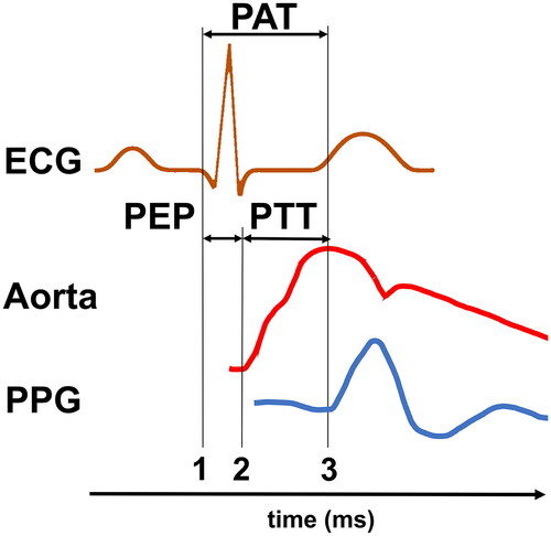
PPG measurements at different locations, specifically the ear, finger, and toe showed that the highest correlation between control BP and PAT-BP was achieved by measuring the toe-PAT [20]. A plausible explanation for this would be the influence of the pre-ejection period (PEP) on cuffless-BP-estimations [21]. PEP is the time difference between PAT and PTT. Latter is defined as the time the pulse wave takes to travel from one measurement point to another. For reasons of easy and precise measurement PTT is most commonly defined as the time between the beginning of blood ejection from the heart into the aorta and the arrival of the mechanical pulse wave in the periphery. PEP equals the time between the start of heart excitation and the beginning of blood ejection (Figure 2 and Table 1) [22]: (7) $$\mathrm{PTT}=\mathrm{PAT}-\mathrm{PEP}$$(7)

Where $\mathrm{PTT}$ = pulse transit time, $\mathrm{PAT}$ = pulse arrival time and $\mathrm{PEP}$ = pre-ejection period

Figure 2. Graphical display of PAT, PEP and PTT. PAT and PTT may vary depending on the starting point, for PAT see also Figure 1. PAT is the time between electrical heart excitation (ECG (1)) and the arrival of the subsequent pulse wave in the periphery (PPG (3)). PTT is the time delay between the onset of a central mechanical wave (here pressure pulse in the aorta (2)) and the arrival of the same pulse wave in the periphery (PPG (3)). PEP is the time between electrical heart excitation (ECG (1)) and the onset of a central mechanical wave (Aorta (2)).

Longer PAT travel times, caused by the increase of distance to the heart when changing the PPG sensor position from ear to finger to toe, result in a smaller impact of PEP on the total measured time. The potential advantages PTT offers over PAT have been recognised in the scientific literature and will further be discussed in the upcoming paragraphs. It must be noted that PAT has a crucial advantage when it comes to its ease of measurement. Therefore, future implementations of PEP correction must not only show their superior BP estimation capabilities but also, and equally importantly, their real-world applicable measurement design.

PEP estimation

Ballistocardiogram for PEP estimation

Ballistocardiograms measure the body’s upward acceleration in response to the downward flow of blood through the descending aorta. This acceleration is measurable and allows the detection of blood ejection from the heart, which directly causes and increases the aortic blood flow. Ballistocardiogram measurements showed the impact of PEP to be relevant for BP estimation (Table 1) [23].

Alternatives to ballistocardiogram measurements for PEP estimation

By using two PPG sensors placed at a fixed distance on the forearm, PWV can be measured directly without using an ECG and therefore circumventing the detection of PEP. It is therefore possible to detect PEP-free PWV estimates, which correlate well with conventional, cuff-based BP measurements. Unfortunately, the existing systems are very prone to measurement artefacts and seem noteworthily hard to administer, even in controlled laboratory settings [24,25]. The impedance cardiography (ICG) is another possible way of measuring PEP. It uses high frequency (HF) and low amplitude electrical pulses to measure changes of electrical conductivity caused by the shift of blood volume into the aorta following blood ejection from the heart [26]. To our knowledge ICGs have not yet been applied for BP estimation in a larger validation study but pose a stable and promising measurement paradigm for future research.

The impact of PEP for future BP-estimation algorithms

The technical difficulties of measuring the PTT directly in different measurement approaches have limited attempts to change the measurement paradigms to address the impact of PEP (Table 1) [24]. Nonetheless, the significance of PEP in measurement precision has been shown convincingly and should not be neglected (Table 1) [21,22,27,28]. Possible options such as an ICG implementation should be further explored to allow for reliable PEP correction.

Improved measurement precision through the usage of additional biomarkers

Models, which include additional physiological parameters, not only offer a higher beat–to–beat measurement precision but may also present themselves to be more robust in real-world applications. Their measurement paradigms do not solely rely on the correct detection and interpretation of one single parameter and are therefore better suited to depict interindividual differences in BP dependencies.

Heart rate

PAT-BP estimations improved when considering the heart rate (HR) as a second model parameter (Table 1) [17]. Models including the HR performed better than multiple different PAT-only models. Synoptical, the focus on BP-estimation-models should be laid on the correct selection of parameters and much less on the precise transfer function. The best performing PAT-BP model considering HR was [29] (8) $$\mathrm{SBP}=a·\mathrm{ }\mathrm{PAT}+b·\mathrm{ }\mathrm{HR}+c$$(8)

Where SBP = systolic BP, HR = heart rate and a, b and c are adjustable parameters, which can be defined based on a larger and more representational dataset.

There also are interesting approaches of estimating the BP only from ECG signals. After a calibration measurement was performed, one group analysed the waveform of the ECG. They showed correlation coefficients of 0.58 and 0.68 for SBP and DBP, respectively, by interpreting ECG signals based on physiological understanding [30].

Photoplethysmogram intensity ratio

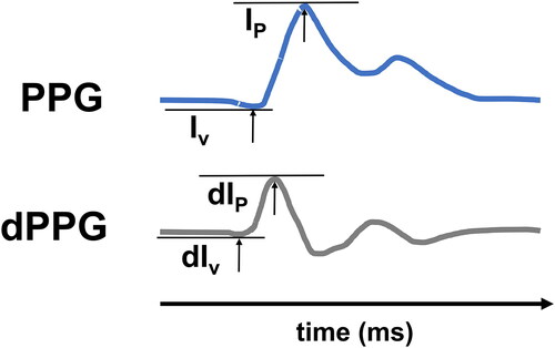
Another promising parameter for improving the precision of PAT for BP estimation is the photoplethysmogram intensity ratio (PIR). PIR is calculated as the ratio of the intensity peak over the intensity valley during one cardiac cycle in the PPG curve (Figure 3).

Figure 3. Upper panel: Calculation of PIR as the difference between peak (I_P) and valley intensity (I_v) of the PPG. Lower panel: First deviation of the PPG signal (dPPG). dPIR is the difference between the peak- (dI_p) and the valley intensity (dI_v).

Integration of PIR into formulas (3) and (4) showed improved accuracy in BP-estimations over several PAT-based models (Table 1) [31,32]. (9) $$\mathrm{PIR}=\mathrm{ }\frac{{\mathrm{Intensity}}_{\mathrm{peak}}}{{\mathrm{Intensity}}_{\mathrm{valley}}}$$(9)

Where PIR = photoplethysmogram intensity ratio, ${\mathrm{Intensity}}_{\mathrm{peak}}$ = maximum intensity in PPG signal during one cardiac cycle, ${\mathrm{Intensity}}_{\mathrm{valley}}$ = minimum intensity in PPG signal during one cardiac cycle.

The most accurate formulas for BP estimation were (Table 1) [32]: (10) $$\mathrm{SBP}=\mathrm{ }{\mathrm{MBP}}_0\mathrm{ }·\mathrm{ }\frac{{\mathrm{PIR}}_0}{\mathrm{PIR}}+\mathrm{ }\frac{2}{3}\mathrm{ }·\mathrm{ }\frac{\mathrm{PIR}}{{\mathrm{PIR}}_0}\mathrm{ }·{\left(\frac{{\mathrm{PAT}}_0}{\mathrm{PAT}}\right)}^2$$(10) (11) $$\mathrm{DBP}=\mathrm{ }{\mathrm{MBP}}_0\mathrm{ }·\mathrm{ }\frac{{\mathrm{PIR}}_0}{\mathrm{PIR}}-\mathrm{ }\frac{1}{3}\mathrm{ }·\mathrm{ }\frac{\mathrm{PIR}}{{\mathrm{PIR}}_0}\mathrm{ }·{\left(\frac{{\mathrm{PAT}}_0}{\mathrm{PAT}}\right)}^2$$(11)

Where $\mathrm{SBP}$ = systolic BP, ${\mathrm{MBP}}_0$ = mean BP at calibration, $\mathrm{PIR}$ = photoplethysmogram intensity ratio,${\mathrm{PIR}}_0$ = $\mathrm{PIR}$ at calibration, $\mathrm{PAT}$ = pulse arrival time and ${\mathrm{PAT}}_0$ = PAT at calibration.

Derivative photoplethysmogram intensity ratio

A problem of PIR measurements is the PPG signal’s susceptibility to artefacts. It has been shown that the usage of PPG’s first derivative (dPIR) is a promising way of counteracting this effect. dPIR is calculated as the ratio of the derived signal’s peak over its valley while being less prone to artefacts. dPIR seems to offer improved accuracy over PIR (Figure 3). (12) $$\mathrm{dPIR}=\mathrm{ }\frac{{\mathrm{dIntesity}}_{\mathrm{peak}}}{{\mathrm{dIntensity}}_{\mathrm{valley}}}$$(12)

Where dPIR = derivative photoplethysmogram intensity ratio, ${\mathrm{dIntesity}}_{\mathrm{peak}}$ = maximum of PPG’s signal derivative in one cardiac cycle and ${\mathrm{dIntensity}}_{\mathrm{valley}}$ = minimum of PPG’s derivative in one cardiac cycle.

The most accurate reported formula in respect to dPIR is (Table 1) [33]: (13) $$\mathrm{SBP}=a\mathrm{ }·\mathrm{PAT}+\frac{b}{\mathrm{dPIR}}+c$$(13) (14) $$\mathrm{DBP}=d\mathrm{ }·\mathrm{PAT}+\mathrm{ }\frac{e}{\mathrm{dPIR}}+f$$(14)

Where SBP = systolic BP PAT = pulse arrival time, DBP = diastolic BP, $\mathrm{dPIR}$ = derivative photoplethysmogram intensity ratio and a, b, c, d, e, and f are adjustable constants (as in formula (8)), which can be defined on a large and representational dataset.

Heart rate power spectrum ratio (HPSR)

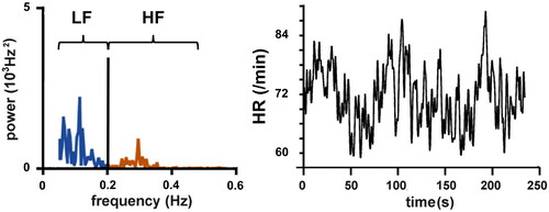
The HPSR correlates with different functional states and pathological alterations in the heart. HPSR is defined as the ratio between the low frequency (LF) and HF heart rate variability components (Figure 4) [34].

Figure 4. HPSR (left panel) of a time series of instantaneous HR (right panel). LF: power in the range between 0.05 and <0.2 Hz, HF: power in the range between 0.2 and 0.5 Hz.

HPSR has been shown to rise when the sympathetic tone is enhanced which is notoriously the case in patients with cardiovascular diseases. This led to the increased interest in HPSR as a possible additional marker for cuffless BP-estimation [35]. The HPSR is therefore, inter alia, highly indicative for cardiovascular strain, caused either by activity or a state of disease [36]. A HPSR enhanced PAT-model showed a close correlation to control-BP values over a multiday measurement analysis [18]: (15) $$\mathrm{HPSR}=\frac{\mathrm{LF}}{\mathrm{HF}}$$(15) (16) $$\mathrm{SBP}=\left({\mathrm{SBP}}_0-\mathrm{ }{\mathrm{DBP}}_0\right)·{\left(\frac{{\mathrm{PAT}}_0}{\mathrm{PAT}}\right)}^2+\mathrm{ }{\mathrm{DBP}}_0\mathrm{ }·\mathrm{ }\frac{\ln \left({\mathrm{PIR}}_0\right)}{{\mathrm{HPSR}}_0}\mathrm{ }·\mathrm{ }\frac{\ln \left(\mathrm{PIR}\right)}{\mathrm{HPSR}}+\mathrm{PIR}+\mathrm{PATV}$$(16) (17) $$\mathrm{DBP}={\mathrm{DBP}}_0\mathrm{ }·\mathrm{ }\frac{\ln \left({\mathrm{PIR}}_0\right)}{{\mathrm{HPSR}}_0}\mathrm{ }·\mathrm{ }\frac{\ln \left(\mathrm{PIR}\right)}{\mathrm{HPSR}}+\mathrm{PIRV}$$(17)

Where $\mathrm{HPSR}$ = heart rate power spectrum ratio, LF = low-frequency heart rate variability components, HF = high-frequency heart rate variability components, ${\mathrm{SBP}}_0,$ ${\mathrm{DBP}}_0,$ ${\mathrm{PAT}}_0,$ ${\mathrm{PIR}}_0,$ ${\mathrm{HPSR}}_0$ are the corresponding values to $\mathrm{SBP}$ = systolic BP, $\mathrm{DBP}$ = diastolic BP, $\mathrm{PAT}$ = pulse arrival time, $\mathrm{PIR}$ = photoplethysmogram intensity ratio and $\mathrm{HPSR}$ at calibration, $\mathrm{PATV}$ = $\mathrm{PAT}$ variability and $\mathrm{PIRV}$ = PIR variability.

Real-world applications

Presently, there is, to the best of our knowledge, only one PAT-based device already tested in 24-h experimental setting. It was validated under the ESH International Protocol in 2015 for short-term use (Table 1) [37]. In 2021, the ESH expressed doubts about the added value of validation of cuffless devices according to the standard protocol for cuff-based devices protocol: If a cuffless device is calibrated shortly before the protocol, it may pass the test even when not providing any meaningful measurement capability [13]. Analogous to cuff-based devices validated according to a protocol for short term use, no reliable statement can be made for cuffless devices about 24-h long term use. For cuffless and cuff-based devices intended for 24-h BP measurements, a more refined validation protocol is required.

Due to the promising results, further investigations into the validity of the PAT-based device have been conducted; 71 patients wore the PAT-based device and a validated cuff-based ABPM simultaneously on different arms during a 24-h BP measurement. Mean differences between both devices were 5.1 mmHg for SBP and 4.2 mmHg for DBP. Daytime-only measurements showed better results with mean differences of 4.2 mmHg for SBP and 3.4 mmHg for DBP. Nocturnal measurements still seemed to be a greater challenge for the cuffless ABPM device under the clinical conditions of this study (12.0 mmHg (SBP) and 9.6 mmHg (DBP)) (Table 1) [38]. These results ask for further optimisation of cuffless ABPM devices to improve measurement precision and real-world applicability.

Avoidable pitfalls in cuffless BP-measurement application

There are pitfalls, which must be avoided for the proper application of cuffless BP measurements. After all, cuffless BP measurement devices derive BP levels through an indirect estimation paradigm. For any indirect measurement, correct calibration is of invaluable importance. Therefore, most devices require a calibration measurement in regular intervals (e.g. 24-h). If the prescribed calibration conditions of the manufacturer are not met, no reliable calibration can be carried out. Calibration measurements are usually comprised of two separate data points: Firstly, a measurement value such as the PAT (+ additional parameters), and secondly, a reference BP-value, most commonly derived from a cuff-based singular measurement. The significance of correct and ideally synchronous calibration measurements has been shown [32]. Failure of correct calibration can lead to intolerable differences in estimated and control BP-values, which can prompt the questionable conclusion of PAT-based BP-estimations being unfit for clinical use (Table 1) [32,39,40].

Future goals for the improvement of PAT-BD-estimations

The PAT/PTT/PWV approach for cuffless ABPM has been developed and improved upon rapidly during the last ten years (Table 1). It is time to progress those ideas more generally into clinical practice and evaluate their reliability under clinical circumstances. The existing clinical validation studies show great promise, even though there are still weaknesses, such as overall measurement accuracy and night-time precision, which need to be further improved in the upcoming years. It has been shown that a special emphasis should be laid on simple and easy to handle calibration and measurement instructions, as a flawed application will lead to extreme measurement imprecision.

Interpretation of model performance

Different cuffless devices are mostly exclusively evaluated by absolute measures (e.g. mean difference between the new model and a reference BP). However, the different devices were tested on different datasets. They vary in intra- and interpersonal variance, for example, dataset of ambulatory 24-h BP measurements may show more BP fluctuations than a laboratory measurement for 30 min at rest. If two different devices, each tested on one of these datasets, retrieve the same mean difference to their reference method, it does not seem reasonable to rate the predictive quality of both devices as equal. To mitigate this, a novel score of relative performance has recently been published: the B-Score. This score allows to evaluate the quality of cuffless BP measurement devices in respect to the dataset it was tested upon. This allows a real comparison between different devices [41].

Open questions

There remain some questions for cuffless BP measurements, which have not yet been completely solved.

First, there is the question about a single model’s capability of appropriately depicting BP-values for different patient collectives. A major advantage of cuff-based ABPMs is their one-for-all approach, which allows measuring almost every given patient with the same methodology. BP estimation via PWV critically depends on the vessels’ stiffness. However, vessel properties vary between different patients. Due to their exceptional hormone status, pregnant women for example have strikingly elastic arteries, while patients with chronic kidney disease are characterised by stiff arteries [42,43]. These differences in vascular properties will lead to different relationships between PWV and BP and therefore may prohibit any given model from correctly estimating BP levels in both groups.

Further, there is the unresolved issue of drug-induced influences on the cardiovascular system, which may alter cardiovascular properties. There have been investigations into the effects of limited groups of drugs and their effects on the cardiovascular system, but in total very few research studies have been conducted on this subject [44].

Devices must show their clinical validity in suitable clinical studies. This is the only way to prove the quality of cuffless BP measurement apparatuses devices and generate trust among clinicians. In a first step, a comparability between different approaches and devices should be created with appropriate tools to better assess which approaches to cuffless BP measurement are most promising, ready for further, clinical validation [13,41,45].

Last, man-made BP estimation models do not aim to be a full representation of the human cardiovascular system but try to estimate singular BP values, which could replace cuff-based measurements. Therefore, these models are not evaluated according to their physiological comprehensibility. They are assessed by their predictive performance on real-world data. It remains to be questioned whether human build algorithms can be complex enough to estimate singular BP values with sufficient precision to make them a viable clinical option for everyday use.

Further research must show its answers to stated open questions and more clearly define and embrace clinical use cases for this exciting new technology (Table 2).

Table 2. Device performances of already tested for 24-h usage and experimental cuffless BP measurement devices.

Suggested metrics	Validated against		Mean Validation	Δ Mean ± SD Validation	Formula	Compared against	Δ Mean ± SD Comparison	Improved	Ref.
Already tested for 24-h application
PAT	osc. sphygmom	SBP: DBP:	134.0 ± 17.3 79.3 ± 11.7	5.1 ± 6.2 4.2 ± 4.4	N/A	N/A	N/A	N/A	38
Experimental improvements in laboratory development
PAT + HR	osc. sphygmom.	SBP:	N/A	1.6 ± 4.4	8	PAT	0.6 ± 5.9	SD	28
PAT + PIR	Finapres	SBP: DBP:	121.1 ± 19.5 68.9 ± 8.2	1.2 ± 5.7 0.4 ± 7.1	10 11	PAT	N/A	Precision	32
PAT + dPIR	Finapres	SBP: DBP:	N/A	3.2 ± 8.0 3.1 ± 4.8	13 14	PAT + PIR	3.5 ± 8.3 3.4 ± 5.2	Stability	33
PAT + PIR + HPSR	sphygmom.	SBP: DBP:	N/A	0.5 ± 7.5 0.8 ± 6.2	16 17	PAT	−1.2 ± 11.2 –0.8 ± 8.4	Precision	18

DBP: diastolic blood pressure; dPIR: derivative photoplethysmogram intensity ratio; HPSR: heart rate power spectrum ratio; HR: heart rate; osc.: oscillometric; PAT: pulse arrival time; PIR: photoplethysmogram intensity ratio; SBP: systolic blood pressure; SD: standard deviation; sphygmom.: sphygmomanometer.

Column 4 provides the differences between the proposed and the validation method. Column 7 provides comparison data chosen by the papers’ authors. All values are provided in the unit of mmHg. Bibliographic reference numbers (Ref.) are provided in the last column.

Machine learning

Computer based systems can be a powerful tool to generate and optimise complex algorithms. Naturally, these ‘machine learning’ systems have been applied to the task of estimating BP values. First, experimental implementations of machine learning models yielded encouraging results. The advantage of machine learning models is that researchers do not have to define concrete mathematical relationships between physiological parameters. Instead, they can focus on selecting appropriate parameters for model creation. The enormous computational power of modern machines then allows to create estimation algorithms with unseen complexity which, in theory, can yield impressive estimation precision. As BP estimation models are evaluated by their predictive performance, it would be negligent to not at least take machine learning tools for BP estimation into consideration.

This part of the review introduces the underlying concepts of machine learning for BP estimation. Our goal is to enable the gain of basic intuitions about the applicability of machine learning concepts for beatto–beat BP measurements, without presupposing any pre-existing knowledge.

Core concepts of machine learning for BP estimation

In general, Machine Learning techniques are a field of computer science which creates a mathematical model of a given real-world system. It achieves this by optimising so-called loss functions over a given dataset [46]. A possible loss function could compute the difference between an estimated BP-value and the reference BP-value, for example, provided by a cuff-based device. A loss function could then average this difference over all given examples in the dataset. Machine Learning algorithms take a predefined input and try to model it so that the algorithm’s output is as close as possible to the ground truth. The easiest example of minimising a loss function is to define a two-dimensional linear regression, which minimises the difference between the linear regression and all measured points.

Machine Learning systems can process more than one input feature and can therefore enable multidimensional regression tasks. Possible features for beat–to–beat BP estimation could comprise PAT, HR, PIR, dPIR, and HPSR, but could be extended to arbitrarily many different features.

There are two main disciplines of Machine Learning: Standard Machine Learning and, perhaps most excitingly, Deep Learning [47]. This review will present examples of both groups being applied to beat–to–beat BP estimation while discussing the possible benefits and limitations of each approach.

Standard machine learning

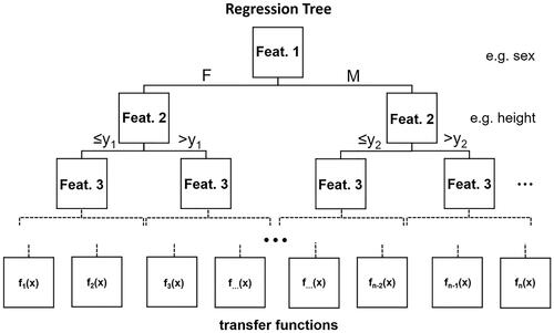
There have been attempts to effectively apply Multiple Linear Regression and Regression Trees to estimate beat–to–beat BP-values. While Multiple Linear Regression relies on the optimisation of multidimensional linear regression tasks, Regression Trees use a network of decision trees to come up with the estimated BP value (Figure 5) [48,49].

Figure 5. Example structure of a Regression Tree. Each layer splits the data based on decision boundaries regarding a single input feature. As an illustration, the first layer splits the data into female and male subsets. The second layer splits the data based on another feature. Regression Trees can have unlimited amounts of decision-layers. The final layer consists of leaves with transfer functions which are used to calculate the final output.

Standard machine learning applications

It has been tried to apply PPG features in Multiple Linear Regression and Regression Tree model training. Those features were comprised of the area under the pulse curve, the pulse rising time from the valley point to the curve’s maximum, and the width of the curve at 25% of the max. The reported results for the trained Regression Tree were substantially better, with results handily beating the performance of any given handcrafted model. Testing the model on a dataset with hypo-, normo- and hypertensive patients led to ascertain the Regression Tree’s validity for only the normotensive group [50].

Another approach for improving machine learning performance is to increase the number of considered input features. Multiple input features can be analysed and reduced into subgroups of the most significant features to train different standard Machine Learning paradigms. The best results have been reported for Ensemble Trees, a specialised form of Regression Trees, and for Gaussian Process Regression, a more sophisticated model resembling the basic concepts of Multiple Linear Regression [48,51,52]. Notably, different models with different input features have been selected for systolic and diastolic BP estimations, as different features seem to offer the highest predictive value. The reported results show a mean absolute error of 3.02 mmHg for SBP and 1.74 mmHg for DBP using a Gaussian process regression derived from a small and controlled dataset [53].

Standard machine learning suitability for BP-estimation?

The real-world applicability of standard Machine Learning techniques for BP estimations remains questionable. While the results seem to be favourable, a lot of concessions had to be made. The generalisability to all patient collectives is still highly in question and would need to be addressed. For example, Khalid et al. recommended the training of multiple Regression Trees for different patient collectives [50]. However, this seems highly inefficient and would provide a lot of uncertainty for patients on the border between two distinct collectives, at which the categorisation into one or the other group could immensely affect the beat–to–beat BP estimation values. After all, there are still the same open questions that remained after assessing the physiological models of insufficient model-complexity and a lack of proper generalisation. Future generations of standard Machine Learning architectures may be powerful enough but still would have to prove their applicability in real-world scenarios.

Deep learning

The rationale for a deep learning approach for BP-estimation

Deep Learning describes a subset of Machine Learning techniques which, due to the increases of computational capacity in the last decade, have become the most powerful tool in the Machine Learning arsenal. Deep Learning models are capable of portraying extremely complicated and complex systems. This capability makes them an especially attractive option for medical applications as biological systems are complex in their multivariability, their non-linear relationships between influencing factors, and the lack of methods for measuring their in vivo dependencies to full extend [54]. BP is the most clinically used surrogate parameter for assessment of the cardiovascular system, one of the most complex biological systems in the human body. It, therefore, seems consistent to test and possibly implement Deep Learning capabilities for beat–to–beat BP estimation tasks.

Successful implementation of deep learning in biomedical applications

The capabilities and benefits of Deep Learning applications have been shown in multiple medical fields. Different kinds of Deep Learning Networks have different strong suits such as Convolutional Neural Networks (CNN) for image processing and Long-Short-Term-Memory (LSTM) models for sequential data. Those concepts will be further described in the following paragraphs. Successful implementations encompass the fields of skin cancer detection, genomic analyses, cellular image analysis, electroencephalogram classification, neuroradiology, and uncountably more [55–61]. It seems like only a matter of time until most if not all medical fields will feel the substantial impact of Deep Learning applications onto their everyday workflow.

Core concepts of deep learning

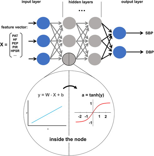
In contrast to ‘standard’ Machine Learning, Deep Learning does not restrain the computer to predefined ‘reasoning principles’. This freedom is fundamental for the unlimited potential of Deep Learning but also complicates the interpretation of its ‘reasoning’. The core concept of Deep Learning is the idea of so-called computational nodes organised in multiple layers. Nodes in the first layer are fed the input features, such as beat–to–beat measured PAT, HR, HPSR, PIR, etc. Then they are multiplied with variable weights and passed through a non-linear activation function. This way each node creates a real number as its output. All nodes in the second layer get all outputs from the first layer and treat them as their input. This procedure can be repeated for multiple layers. For regression tasks, such as beat–to–beat BP estimation, the last layer is comprised of only one node, which takes all outputs of the second to last layer as inputs and itself outputs a real number, which is treated as the model’s prediction based on the input features. A loss function is defined which determines the difference between predicted and true values. The Deep Learning model tries to optimise its weights in every node to minimise this loss function and therefore minimise the difference between its predictions and the ground truth. Correct choice of an appropriate loss function can guarantee the model minimising the measurement error in every individual patient. Therefore, it is trained by calculating the average loss over a training set, adjusting the weights slightly, recalculating the average loss, and so forth. Training of Deep Learning Networks is computationally very expensive and a highly iterative process in which the programmers must finetune multiple so-called hyperparameters, which affect the performance of the model. The resulting model can then be tested on a dataset it has not seen during training and, if the performance is good enough, can be used to predict the desired beat–to–beat BP values in real life for individual patients (Figure 6) [54,62].

Figure 6. Schematic structure of Deep Learning architecture. Input features are fed into the model as a vector and passed into the hidden layers. Hidden layer nodes take the inputs and run them through two calculations (inside the node). First, a multilinear equation takes a weight vector (W), the input vector (X), and a bias term (b) to calculate a temporary variable (y). This variable is then fed into a non-linear activation function (e.g. tanh) to calculate the node’s output (a). All nodes within a layer pass their output to all nodes in the following layer (arrows) which stack them into a vector and treat them as their input vector. The final hidden layer passes its activations (a) into the output layer, which in this case has two nodes (for SBP and DBP). Nodes in the output layer do not have an activation function and output the result of their linear function (y). The model is trained by optimising each node’s W and b to minimise the difference between a ground truth presented by the training dataset and the models corresponding predictions.

CNN models

CNNs can take pictures or multidimensional input data in general, as input features and determine all relevant components analysing them. Basically, pictures are two-dimensional arrays of pixels which have different values for their colour channels, such as red, green and blue for standard picture formats. While most Deep Learning Networks are dependent on unidimensional input data, such as measured values at a certain time point, CNNs can intake those arrays as a whole and derive spatial intuition about the picture’s contents. CNNs application has had great success in multiple medical fields [59–61].

With the goal of applying this technology for beat–to–beat BP estimation, ECG- and PPG-curves were fed into a CNN. It was then trained on a dataset comprised of intensive care patients. While the model scored remarkable measurement precision, the retraining of the model with multiple calibration values for every new patient was suggested. This makes the computational load for every given patient extremely high and deems this approach highly inelegant as it involves a large amount of setup work, which is unfeasible in clinical reality [63]. Transferring this approach to the real world may be conceivable for patients in a hospital ward with an adjacent datacenter or commercial providers with provided cloud computing. However, it is unrealistic for on-site, real-time computing, wearable ABPMs [49].

Further investigation of CNNs and their capabilities for BP measurements should be conducted as there is the chance of creating a generalising CNN, which would not depend on model retraining.

LSTM models

Another tested Deep Learning architecture is LSTM models. LSTM models do not themselves analyse pictures to retrieve needed information but take predefined features as input. Their advantage is their capability of taking multiple sets of input, remembering the most important ones, and then feed forward the information into a decision network [64]. LSTM models have already shown their impressive capability of predicting heart failure and therefore seem highly suitable for modelling the cardiovascular system in other sequential domains, such as beat–to–beat BP time-series [65]. LSTM models designed to input multiple instances of input features like ECG- and PPG-features and combining them into output beat–to–beat BP values for each systolic and diastolic values are described in the literature. Practically speaking, the model intakes information about multiple heart cycles remembers the most important of those features and makes predictions based on them. Hopeful results have been reported from deep learning architectures with the ability to estimate beat–to–beat BP for individual patients [66,67].

Limitations of CNNs and LSTM-models

Just like CNNs, LSTM-models are very computationally expensive. They therefore require a lot of computational capability for portable devices as well as sufficient battery capacity. It is very questionable whether a wearable LSTM based ABPM-device is feasible and even if, whether it is economically reasonable with today’s technology. One disadvantage of the LSTM approach is the limitation of resulting BP values. While conventional cuffless BP measurement systems allow a true ‘beat–to–beat’ BP estimation a LSTM takes a certain number of heart cycles (e.g. ten) into account. The solution for this are ‘lagging LSTM-models’, which take ten heart cycles, estimates the BP, drop the oldest heart-cycle features, and add the newest to generate the next batch of 10 heart cycles. A ‘lagging LSTM-model’ is most certainly not feasible for any real-time and on-site computing, wearable 24 h-device based on available technology. The real-world advantages of one-site and real-time computability are obvious, as they enable the development of true user-based measurement devices, which could revolutionise how the medical society thinks about cardiovascular diagnosis and early disease detection. Increasing computational power and battery capacities will push the boundaries of possible on-site device capabilities. Until then, development of a well-functioning, cloud-computed Deep Learning model may lead to real-world ready, on-site solutions in the foreseeable future.

Further, all Deep Learning approaches must show their validity for many diverse patient cohorts in different age groups and with different health conditions. No such analysis has yet been conducted up to this point. There is no reliable metric allowing the comparison of beat–to–beat BP estimation model performances over multiple datasets. The development of such metrics and successful implementation on various patient cohorts are prerequisites for the development of truly generalised beat–to–beat BP estimation algorithms which can be ready for large-scare clinical use.

A major concern for Deep Learning models is the lack of a real ground truth which is needed to ideally train the models. Ground truth values would only be accessible in intra-arterial measurement scenarios as cuff-based measurement paradigms lack precision compared to direct, intraarterial measurements [68]. Those catheter-based measurements are standard procedures in intensive care units, which would allow for easy collection of data samples, but they present one major drawback: Intensive care patients are in general immobile, sick and are medically prevented from large deviations in their BP levels. Deep Learning models rely on diverse and representative training data, but there is no rational way of including intraarterial BP measurements into the training data, given the practical hindrances and risk concerns associated with intra-arterial BP measurements [69]. The best practical approach is to collect as many cuff-based BP values as possible and correlate them with other recorded biomarkers. This approach is limited by the inaccuracies and methodological weaknesses of cuff-based BP measurements. The rigorous detection of measurement artefacts during cuff-based BP measurements is a prerequisite for the collection of datasets of acceptable measurement quality. Still, any given Deep Learning model will, trained on such datasets, not measure the real, intraarterial BP, but will estimate the corresponding cuff-based value. As cuff-based devices are considered suitable for 24 h-ABPMs and as the rigorous exclusion of flawed training data will lead to a better estimation of real BP-levels, compared to standard and uncorrected cuff-based measurements, it is reasonable to predict Deep Learning applications to handily become precise enough for clinical use [2]. Notably, this precision has to and will be assessed based on a models reliability for singular measurements in individual patients and not for correlations with the overall cohort mean.

The possible intersection between physiological and deep learning models

A new and promising concept of improving cuffless BP estimation is to strive for combining takeaways from physiological understanding and feed them into Deep Learning models. Clinicians’ confidence in cuffless BP estimation models will rise when the input parameters are understandable to them. Therefore, selecting physiologically comprehensible parameters for Deep Learning applications can improve both estimation performance and model acceptance. While models fed with raw input signals have shown great experimental measurement precision, they also are an inscrutable black box. Models relying on parameters shown to be predictive in physiological research articles such as PAT, HR, dPIR and HRSP are more likely to be accepted by the clinical community.

Additionally, further physiologically intuitive parameters can be incorporated in a Deep Learning model, which would pose a very difficult task for man-made models. Such parameters could be the patients’ age, height, weight, and sex, to represent interpersonal differences. Even the time of measurement, to represent typical circadian effects, or even more advanced metrics like room temperature or elevation above sea level could be included. All these parameters can have a large influence on the cardiovascular system, with different effect sizes on different patients. Deep Learning models are suited to detect those differences and make precise beat–to–beat BP predictions for individual patients.

Ultimately, combining physiological understanding and Deep Learning models would be chance combine the best of two worlds.

Conclusion

After all, the field of cuffless and continuous beat-to–beat BP measurement is set for a bright future. Two approaches have solidified themselves as possible ways of finally promoting cuffless techniques into clinical viability.

On the one hand, models based on physiological parameters have been greatly improved upon in recent years. While a commercially available device shows promising first validation results, even more complex transfer functions are being developed. In the future, the inclusion of additional parameters, such as the HR, PIR, dPIR, PEP or HPSR, seems to be an exciting option to further increase beat–to–beat BP estimation precision. As datasets for model development and validation are growing, more refined and fine-tuned models will enter the market.

On the other hand, researchers are trying to unleash the groundbreaking capabilities of Deep Learning architectures for medical applications and exert them for beat–to–beat BP estimation. Those models can intake raw or preprocessed data and studies have shown inconceivably high levels of measurement precision in early state development. Their future application to the field of beat–to–beat BP estimation and first real-world applications are to be observed with anticipation.

Last, there is very much the possibility that these seemingly diametrically opposed approaches can be brought together to a symbiotic interaction in which the gained insights of physiological models are used to enhance a Deep Learning based beat–to–beat BP estimation concept. As it is often the case in medical or biological systems, models unifying insights from multiple and very different academic disciplines tend to come closer to the unmatched complexity of nature.

A first and very straightforward approach would be to use preprocessed parameters shown to work well in PAT-based models and carefully inject them into a sophisticated Deep Learning architecture. This approach could possibly enable a future of cuffless and continuous beat–to–beat BP estimation, while still preserving physiological traceability of model input features.

However, further research is necessary to increase accuracy and practicability of cuffless devices. This will improve doctor’s confidence in cuffless devices and enable to establish them in everyday clinical practice.

Acknowledgement

The authors thank Dr. Oleg Anosov and Laura Josefa Dippel for helpful discussions and comments during development of this work.

Disclosure statement

T.L.B. and A.P. are advisors for SOMNOmedics on blood pressure measurement. N.P. declares no competing interests.

References

- Williams B, Mancia G, Spiering W, ESC Scientific Document Group, et al. ESC/ESH guidelines for the management of arterial hypertension. Eur Heart J. 2018;39(33):3021–3104.
- Whelton PK, Carey RM, Aronow WS, et al. ACC/AHA/AAPA/ABC/ACPM/AGS/APhA/ASH/ASPC/NMA/PCNA guideline for the prevention, detection, evaluation, and management of high blood pressure in adults a report of the American College of Cardiology/American Heart Association Task Force on Clinical practice guidelines. Hypertension 2017;71:E13–115. https://doi.org/10.1161/HYP.0000000000000065.
- Agarwal R, Light RP. The effect of measuring ambulatory blood pressure on nighttime sleep and daytime activity - Implications for dipping. CJASN. 2010;5(2):281–285.
- Sherwood A, Hill LK, Blumenthal JA, et al. The effects of ambulatory blood pressure monitoring on sleep quality in men and women with hypertension: Dipper vs. Nondipper and race differences. Am J Hypertens. 2019;32(1):54–60.
- Davies RJO, Jenkins NE, Stradling JR. Effect of measuring ambulatory blood pressure on sleep and on blood pressure during sleep. BMJ. 1994;308(6932):820–823.
- Mancia G, Sega R, Bravi C, et al. Ambulatory blood pressure normality: Results from the PAMELA study. J Hypertens. 1995;13(12):1377–1390.
- Fagard RH, Celis H, Thijs L, et al. Daytime and nighttime blood pressure as predictors of death and cause-specific cardiovascular events in hypertension. Hypertension. 2008;51(1):55–61.
- Sega R, Facchetti R, Bombelli M, et al. Prognostic value of ambulatory and home blood pressures compared with office blood pressure in the general population: Follow-up results from the pressioni arteriose monitorate e loro associazioni (PAMELA) study. Circulation. 2005;111(14):1777–1783.
- Gavriilaki M, Anyfanti P, Nikolaidou B, et al. Nighttime dipping status and risk of cardiovascular events in patients with untreated hypertension: a systematic review and Meta‐analysis. J Clin Hypertens (Greenwich). 2020;22(11):1951–1959.
- Raymaekers V, Brenard C, Hermans L, et al. How to reliably diagnose arterial hypertension: lessons from 24 h blood pressure monitoring. Blood Press. 2019;28(2):93–98.
- Stevens SL, Wood S, Koshiaris C, et al. Blood pressure variability and cardiovascular disease: Systematic review and Meta-analysis. BMJ. 2016;354:i4098.
- Parati G, Stergiou GS, Dolan E, et al. Blood pressure variability: clinical relevance and application. J Clin Hypertens. 2018;20(7):1133–1137.
- Stergiou GS, Mukkamala R, Avolio A, et al. Cuffless blood pressure measuring devices: review and statement by the european society of hypertension working group on blood pressure monitoring and cardiovascular variability. J Hypertens. 2022;40(8):1449–1460.
- Stergiou GS, Palatini P, Parati G, European Society of Hypertension Council and the European Society of Hypertension Working Group on Blood Pressure Monitoring and Cardiovascular Variability, et al. 2021 European society of hypertension practice guidelines for office and out-of-office blood pressure measurement. J Hypertens. 2021;39(7):1293–1302.
- Callaghan FJ, Babbs CF, Bourland JD, et al. The relationship between arterial pulse-wave velocity and pulse frequency at different pressures. J Med Eng Technol. 1984;8(1):15–18.
- Gesche H, Grosskurth D, Küchler G, et al. Continuous blood pressure measurement by using the pulse transit time: Comparison to a cuff-based method. Eur J Appl Physiol. 2012;112(1):309–315.
- Wang R, Jia W, Mao ZH, et al. Cuff-free blood pressure estimation using pulse transit time and heart rate. International Conference on Signal Processing Proceedings, ICSP, 2015 January, Institute of Electrical and Electronics Engineers Inc.; 2014. p. 115–8. https://doi.org/10.1109/ICOSP.2014.7014980.
- Chen Y, Shi S, Liu YK, et al. Cuffless blood-pressure estimation method using a heart-rate variability-derived parameter. Physiol. Meas. 2018;39(9):095002.
- Zheng YL, Yan BP, Zhang YT, et al. An armband wearable device for overnight and cuff-less blood pressure measurement. IEEE Trans Biomed Eng. 2014;61(7):2179–2186.
- Block RC, Yavarimanesh M, Natarajan K, et al. Conventional pulse transit times as markers of blood pressure changes in humans. Sci Rep. 2020;10(1):16373.
- Newlin DB. Relationships ol pulse transmission times to pre‐ejection period and blood pressure. Psychophysiology. 1981;18(3):316–321.
- Beutel F, van Hoof C, Rottenberg X, et al. Pulse arrival time segmentation into cardiac and vascular Intervals - Implications for pulse wave velocity and blood pressure estimation. IEEE Trans Biomed Eng. 2021;68(9):2810–2820.
- Yousefian P, Shin S, Mousavi A, et al. The potential of wearable limb ballistocardiogram in blood pressure monitoring via pulse transit time. Sci Rep. 2019;9(1):10666.
- Wang Y, Liu Z, Ma S. Cuff-less blood pressure measurement from dual-channel photoplethysmographic signals via peripheral pulse transit time with singular spectrum analysis. Physiol Meas. 2018;39(2):025010.
- Chan G, Cooper R, Hosanee M, et al. Multi-Site photoplethysmography technology for blood pressure assessment: Challenges and recommendations. J Clin Med. 2019;8:1827.
- DeMarzo AP. Clinical use of impedance cardiography for hemodynamic assessment of early cardiovascular disease and management of hypertension. High Blood Press Cardiovasc Prev. 2020;27(3):203–213.
- Zhang G, Cottrell AC, Henry IC, et al. Assessment of pre-ejection period in ambulatory subjects using seismocardiogram in a wearable blood pressure monitor. Proceedings of the Annual International Conference of the IEEE Engineering in Medicine and Biology Society, EMBS, 2016 October, Institute of Electrical and Electronics Engineers Inc.; 2016. p. 3386–9. https://doi.org/10.1109/EMBC.2016.7591454.
- Muehlsteff J, Aubert XL, Schuett M. Cuffless estimation of systolic blood pressure for short effort bicycle tests: the prominent role of the pre-ejection period. Annual International Conference of the IEEE Engineering in Medicine and Biology - Proceedings, 2006. p. 5088–92. https://doi.org/10.1109/IEMBS.2006.260275.
- Zhang Q, Zhou D, Zeng X. Highly wearable cuff-less blood pressure and heart rate monitoring with single-arm electrocardiogram and photoplethysmogram signals. Biomed Eng OnLine. 2017;16(1):23.
- Scalise F, Margonato D, Sole A, et al. Ambulatory blood pressure monitoring by a novel cuffless device: a pilot study. Blood Press. 2020;29(6):375–381.
- Ding XR, Zhang YT, Liu J, et al. Continuous cuffless blood pressure estimation using pulse transit time and photoplethysmogram intensity ratio. IEEE Trans Biomed Eng. 2016;63(5):964–972.
- Ding X, Yan BP, Zhang YT, et al. Pulse transit time based continuous cuffless blood pressure estimation: a new extension and A comprehensive evaluation. Sci Rep. 2017;7(1):11554.
- Lin WH, Wang H, Samuel OW, et al. Using a new PPG indicator to increase the accuracy of PTT-based continuous cuffless blood pressure estimation. Proceedings of the Annual International Conference of the IEEE Engineering in Medicine and Biology Society, EMBS, 2017, Institute of Electrical and Electronics Engineers Inc.; 2017. p. 738–41. https://doi.org/10.1109/EMBC.2017.8036930.
- Ori Z, Monir G, Weiss J, et al. Heart rate variability: Frequency domain analysis. Cardiol Clin. 1992;10(3):499–537.
- Akselrod S, Gordon D, Ubel FA, et al. Power spectrum analysis of heart rate fluctuation: a quantitative probe of beat-to-beat cardiovascular control. Science. 1981;213(4504):220–222.
- Zhang Y, Zhou B, Qiu J, et al. Heart rate variability changes in patients with panic disorder. J Affect Disord. 2020;267:297–306.
- Bilo G, Zorzi C, Ochoa Munera JE, et al. Validation of the Somnotouch-NIBP noninvasive continuous blood pressure monitor according to the european society of hypertension international protocol revision 2010. Blood Press Monit. 2015;20(5):291–294.
- Socrates T, Krisai P, Vischer AS, et al. Improved agreement and diagnostic accuracy of a cuffless 24-h blood pressure measurement device in clinical practice. Sci Rep. 2021;11(1):1143.
- Moharram MA, Wilson LC, Williams MJ, et al. Beat-to-beat blood pressure measurement using a cuffless device does not accurately reflect invasive blood pressure. Int J Cardiol Hypertens. 2020;5:100030.
- Patzak A. Measuring blood pressure by a cuffless device using the pulse transit time. Int J Cardiol Hypertens. 2021;8:100072.
- Bothe TL, Patzak A, Pilz N. The B-Score is a novel metric for measuring the true performance of blood pressure estimation models. Sci Rep. 2022;12(1):12173.
- Chen SC, Huang JC, Su HM, et al. Prognostic cardiovascular markers in chronic kidney disease. Kidney Blood Press Res. 2018;43(4):1388–1407.
- Ulusoy RE, Demiralp E, Kirilmaz A, et al. Aortic elastic properties in young pregnant women. Heart Vessels. 2006;21(1):38–41.
- Batzias K, Antonopoulos AS, Oikonomou E, et al. Effects of newer antidiabetic drugs on endothelial function and arterial stiffness: a systematic review and meta-analysis. Journal of Diabetes Research. 2018;2018:1–10.
- Burnier M, Kjeldsen SE, Narkiewicz K, et al. Cuff-less measurements of blood pressure: are we ready for a change? Blood Press. 2021;30(4):205–207.
- Deo RC. Machine learning in medicine. Circulation. 2015;132(20):1920–1930.
- Goecks J, Jalili V, Heiser LM, et al. How machine learning will transform biomedicine. Cell. 2020;181(1):92–101.
- Fernández-Delgado M, Sirsat MS, Cernadas E, et al. An extensive experimental survey of regression methods. Neural Netw. 2019;111:11–34.
- Marill KA. Advanced statistics: Linear regression, part II: Multiple linear regression. Acad Emerg Med. 2004;11(1):94–102.
- Khalid SG, Zhang J, Chen F, et al. Blood pressure estimation using photoplethysmography only: Comparison between different machine learning approaches. J Healthc Eng. 2018;2018:1548647.
- Seeger M. Gaussian processes for machine learning. Int J Neural Syst. 2004;14(2):69–106.
- Banerjee M, Reynolds E, Andersson HB, et al. Tree-based analysis: a practical approach to create clinical decision-making tools. Circ Cardiovasc Qual Outcomes. 2019;12(5):e000056.
- Chowdhury MH, Shuzan MNI, Chowdhury MEH, et al. Estimating blood pressure from the photoplethysmogram signal and demographic features using machine learning techniques. Sensors (Switzerland). 2020;20(11):3127.
- Esteva A, Robicquet A, Ramsundar B, et al. A guide to deep learning in healthcare. Nat Med. 2019;25(1):24–29.
- Zaharchuk G, Gong E, Wintermark M, et al. Deep learning in neuroradiology. AJNR Am J Neuroradiol. 2018;39(10):1776–1784.
- Moen E, Bannon D, Kudo T, et al. Deep learning for cellular image analysis. Nat Methods. 2019;16(12):1233–1246.
- Zou J, Huss M, Abid A, et al. A primer on deep learning in genomics. Nat Genet. 2019;51(1):12–18.
- Munir K, Elahi H, Ayub A, et al. Cancer diagnosis using deep learning: a bibliographic review. Cancers (Basel). 2019;11(9):1235.
- Esteva A, Kuprel B, Novoa RA, et al. Dermatologist-level classification of skin cancer with deep neural networks. Nature. 2017;542(7639):115–118.
- Yamashita R, Nishio M, Do RKG, et al. Convolutional neural networks: an overview and application in radiology. Insights Imaging. 2018;9(4):611–629.
- Anwar SM, Majid M, Qayyum A, et al. Medical image analysis using convolutional neural networks: a review. J Med Syst. 2018;42:1–13.
- Cao C, Liu F, Tan H, et al. Deep learning and its applications in biomedicine. Genom Proteom Bioinformat. 2018;16(1):17–32.
- Yan C, Li Z, Zhao W, et al. Novel deep convolutional neural network for cuff-less blood pressure measurement using ECG and PPG signals. Proceedings of the Annual International Conference of the IEEE Engineering in Medicine and Biology Society, EMBS, Institute of Electrical and Electronics Engineers Inc.; 2019. p. 1917–20. https://doi.org/10.1109/EMBC.2019.8857108.
- Yu Y, Si X, Hu C, et al. A review of recurrent neural networks: Lstm cells and network architectures. Neural Comput. 2019;31(7):1235–1270.
- Maragatham G, Devi S. LSTM model for prediction of heart failure in big data. J Med Syst. 2019;43(5):111.
- Lee D, Kwon H, Son D, et al. Beat-to-beat continuous blood pressure estimation using bidirectional long short-term memory network. Sensors. 2020;21(1):96.
- Li YH, Harfiya LN, Purwandari K, et al. Real-time cuffless continuous blood pressure estimation using deep learning model. Sensors. 2020;20(19):5606–5619.
- Kim SH, Lilot M, Sidhu KS, et al. Accuracy and precision of continuous noninvasive arterial pressure monitoring compared with invasive arterial pressure: a systematic review and Meta-analysis. Anesthesiology. 2014;120(5):1080–1097.
- Abbott TEF, Howell S, Pearse RM, et al. Mode of blood pressure monitoring and morbidity after noncardiac surgery A prospective multicentre observational cohort study. Eur J Anaesthesiol. 2021;38(5):468–476.