Potential of hyperspectral-based geochemical predictions with neural networks for strategic and regional exploration improvement

Abstract

This paper summarises an evaluation of the application of artificial intelligence to hyperspectral drill-core scans for more effective mineral exploration. The dataset used was based on publicly available core scans and related geochemical analysis from Australia. Prior to unification, a detailed quality assessment of the geochemical data was undertaken. Special focus was paid to gold, silver, copper, iron, uranium, nickel, lead, tin, antimony, arsenic and bismuth contents. The dataset was labelled with defined ore grades related to economic cutoff values. The impact on predictions of different setups is related to the amounts of data used for learning, data design and implementation of the geological domains. Based on 1-metre bins, the results from more than 700 km of drill cores were used and analysed with the potential for geological exploration in different scenarios discussed. The results indicate the enormous potential of the use of hyperspectral scans in combination with artificial intelligence for the development of exploration scenarios and to provide support for exploration geologists and target detection. The application of predictors on scanned drill cores from Australia also indicates mineralised zones that have not been analysed chemically for all metals above economic cutoffs. This result shows the enormous potential of the approach for strategic exploration but also mining operations. Prediction of geochemical concentrations for gold, copper and iron based on a neural network in drill cores is possible. Using mineral abundances from hyperspectral core scans as learning records, and existing elemental geochemical analyses as labels, the predictions are given with an accuracy of better than 80–90%.

KEY POINTS

1. The trained artificial intelligence system has for the first time enabled direct estimation of metal grades from hyperspectral scans.

2. It also shows potential for applications to analyse airborne hyperspectral data for direct mapping of metal grades.

3. Finally, it may pave the way for better plant management by the usage of hyperspectral data for direct grade estimations in operational mining and ore sorting.

Keywords:

• exploration
• drill core
• hyperspectral
• core scan
• artificial intelligence
• neural network
• metals

Introduction

This study evaluates the potential of a specially designed neural network for the prediction of geochemical properties in drill cores based on hyperspectral core scans. The importance of different parameters to the training of the neural network is assessed for the prediction of geochemical properties. The evaluation is set to support the implementation on multi-dimensional prediction methods of artificial intelligence for supporting operational and strategic tasks in geological exploration using hyperspectral drill-core information.

Motivation

In an exploration scenario, mapping of minerals using hyperspectral scans of drill cores, on the one hand, and geochemical analysis of sampled core segments, on the other hand, are two tools for geologists to identify areas with higher grades of targeted ore, and alteration and mineralisation zones (Moon et al., 2006). Arne (2014), Lampinen et al. (2016) and Sun et al. (2019) demonstrated the relationship of minerals mapped via hyperspectral analysis and geochemical assays to describe geological settings. Typically, owing to high costs, geologists select the locations of geochemical analysis is limited and may be biased by their knowledge and experience; reduced geochemical sampling might lead to relevant segments of core being overlooked in the design of the exploration model. The specially designed neural network can bridge this gap between complete core information from hyperspectral scanning and the incomplete geochemical information. The evaluation of different setups provides an understanding of the impact of different implementation parameters on the results and therefore the usability of the workflow in geological exploration.

Literature review and theoretical background

Improvements in knowledge of geology have developed differently over the decades. While the documenting of geological properties in field studies still plays a major role, the application of new geophysical and spectral investigation methods combined with the implementation of computational and mathematical fundamental knowledge behind geological theories is rapidly increasing (Dramsch, 2020). Machine automation has become an important tool to enhance geological understanding, especially in geophysics. Modern deep learning hardware and methods combined with the availability of big data in geological archives has opened new opportunities for analysing complex datasets (Geng, 2016; Karpatne et al., 2020). Kulesza et al. (2014) and Roh et al. (2018) highlighted the importance of structuring data for artificial intelligence and labelling. Grade of ore, geophysical well-log properties and sharp fault detection on seismic images are examples of successful labelling in geological applications. Caté et al. (2017) used machine-learning algorithms connecting petrophysical properties with gold-bearing intervals to improve the selection of gold intervals for assay sampling. Acosta et al. (2020) integrated hyperspectral and geochemical data via a superpixel-based machine-learning classification that gave a model improvement of 20% in the accuracy of results against an individuals analysis of the datasets on the pixel.

Rodger and Laukamp (2021) developed an approach using hyperspectral data to predict geochemical quantities using a trained workflow consisting of a non-negative matrix function step for data reduction and a random forest regression with an accuracy for predictions of up to 0.96 for R². Their method was based on the use of reflectance spectra between 400 and 25 000 nm. In a different approach, Eichstaedt et al. (2020) used airborne spectral data from a specially designed test field with controlled coverage of clay containing target materials to derive quantitative estimations. Fouedjio et al. (2018) highlighted the possibilities of geostatistical methods to keep spatial relations between drill holes as part of geological domain definitions coupled with geochemical measurements.

The methodological research on convolutional neural networks and the minimum requirements and best setups to achieve learning vary widely and reflect problems in the preparation of suitable datasets (Du et al., 2018). The increase in sample numbers is important for increased accuracies of the network predictions. The design, as well as the strategies applied to the conditioning of the datasets, is of major importance for the performance of the neural networks (Bao, 2019; Neyshabur et al., 2017).

The following evaluation is focused on the potential impact of using a convolutional neural network with mineral abundances derived from hyperspectral data, and the stability of the results. The network architecture is described in detail in Eichstaedt et al. (2022). This paper focusses on the performance of different methods for the evaluation of drill-core scans.

Geological context and data

Australia has a rich history of research in geological and ore-forming processes, and exploration has led to expertise in many mineral and metal commodities. The Australian continent is prospective for bauxite (aluminium ore), iron ore, lithium, gold, lead, diamonds, rare earth elements, uranium, zinc, manganese, antimony, nickel, silver, cobalt, copper and tin from over 350 operating mines (Geoscience Australia, 2021; Jaques et al., 2002). The intense exploration programs by the well-established mining industry and Australian State and Territories government agencies have cumulated in more than 3.2 million drill holes with thousands hyperspectrally scanned under the framework of the AuScope National Virtual Core Library (AuScope, 2020). Approximately 70 million records of geochemical analyses are available to the public by individual states websites and geological surveys.

Material

To train a specialised neural network, hyperspectral drill-core data collected by means of HyLogger (Schodlok et al., 2016) and the mineralogical interpretations derived from the hyperspectral data using matching algorithms, such as The Spectral Assistant (Berman et al., 2017), were collected from AuScope and Australian State and Territories. The acquired data were processed with The Spectral Geologist (TSG^®) software provided by Commonwealth Scientific Industrial Research Organisation (CSIRO). We used pre-interpreted spectral analyses of minerals in the visible and infrared, short-wave infrared and thermal longwave bands (VNIR/SWIR/TIR) (Green, 2020; Leybourne et al., 2013). Mineral species were used for the development of the neural network. The NVCL and CSIRO studies have shown that the accuracy of The Spectral Assistant (TSA) at the mineral species level is lower than the results at the mineral group level (Laukamp, personal communication). Data were captured as relative abundances in percentage per 1-metre intervals from over 2700 drill holes with depth ranges between 60 and 4400 m. TSA, which is a general unmixing algorithm, was used to identify selected minerals and calculate abundances for SWIR and TIR in 1-metre intervals. These abundances for each spectrum are calculated proportions of the library spectra required to best fit the measured spectrum. In this study, SWIR and TIR responses were matched to mineral libraries using the scalar information of system TSA (sTSAT)-based spectral reflectance measurements (Green, 2020; Schodlok et al., 2016). The SWIR wavelength only identifies hydrous silicates and carbonates. Since 2017, the TSA interpretation for the TIR, the sTSAT, has been progressively replaced by the joint Constrained Least Squares (jCLST) algorithms, another unmixing classifier (Green, 2020). jCLST interprets the TIR data using the results from the SWIR spectra and scalars focused on selected features in the visible near infrared (VNIR) and TIR wavelengths (Green, 2020). Up to December 2021, a total of 2709 drill holes with 927 206 m sampling were collected for SWIR, and 876 857 m for TIR.

For the development of the neural network, geochemical assays of the elements, gold, silver, copper, iron, uranium, nickel, lead, tin, antimony, arsenic and bismuth were extracted. Of the 70 million geochemical records, 110 000 were matched with 703 250 one-metre intervals of the TIR/SWIR hyperspectral measurements and used for development, training and evaluation of the neural network. In the geochemical samples, same-depth intervals of the hyperspectral 1-metre bins were rounded to the majority covered by the spectral bin. Geochemical samples cover a 2-metre segment of core, so the geochemical record was duplicated for both covered hyperspectral bins.

Methodology

The geochemical dataset for the neural network was labelled based on threshold limits given in Table 1. The thresholds for the classes focused on typical values for exploration and additionally on the requirements for balancing the data amounts to ensure a good performance of neural networks. For the evaluation, two, three and four ore-grade classes were implemented, starting on top grades. Above and below the threshold, the same amount of data has been randomly sampled to achieve a balanced learning data pool.

Table 1. Overview of accuracies achieved in a two-class learning approach with the neural network based on the 20% test dataset.

Element	Threshold equals or above	Training samples above threshold	Accuracy of prediction based on confusion matrix 20% test dataset percentage correct allocated
Ag	0.5 ppm	21 400	80.95
Au	0.17 ppm	16 245	81.86
	0.09 ppm	22 619	80.02
Fe	36.50 wt%	5350	94.03
	21.20 wt%	10 700	92.19
	12.80 wt%	16 050	91.38
	9.20 wt%	21 400	88.30
Cu	3890 ppm	10 700	83.75
	2000 ppm	16 050	81.13
	1150 ppm	21 400	79.59
U	10 ppm	5350	88.93
	4.27 ppm	10 700	88.83
	0.881 ppm	16 050	89.27
Ni	22 ppm	3300	92.60
Pb	5 ppm	5350	90.28
Zn	68 ppm	5350	91.57
Sb	0.25 ppm	5350	93.68
As	6 ppm	5350	92.62
Bi	0.12 ppm	5350	94.90

The thresholds are defined by the upper percentiles of the geochemical records in the database.

For this work, a specially developed neural network was tested with the aim to evaluate the impact of specific parameters on the geochemical prediction results. To evaluate the accuracy of the methodology, 60% of the label set of 110 000 geochemical records were randomly chosen for learning, 20% for verification and 20% for independent testing. All classes of the test dataset were complete, with no missing values in any variable or outliers.

The developed neural network can be classified as a convolutional neural network. It employs convolutional layers as filters (kernel) to transform data into a randomised number of values in a grid (O’Shea & Nash, 2015). The CNN model base was built prior to this experiment in the context of Dimap’s chemoin-format and geological studies. It has proven to be more stable and efficient than other widely used convolutional networks and enables predictions from independent individual multiple-value datasets (Eichstaedt et al., 2020). These investigations demonstrate that these networks have enough degrees of freedom and a suitable capacity for the analysis of the specific kinds of data, especially considering the necessary compromise between accuracy and generalisation error. For the network, the Rectified Linear Unit was applied as an activation function and Softmax for the multi-class classification to ensure the output probabilities (predictor values) for the classes add up to 1. The neural network was realised using Keras and TensorFlow. The training was conducted over 200 epochs with 400 features and data augmentation in one direction, to ensure a stable and steady learning environment. Figure 1 shows the general design of the neural network. The results of each test were measured in a confusion matrix, which showed the correct and incorrect predicted classes for the 20% test dataset.

Figure 1. Schematic model illustration of the neural network designed for the evaluation (Eichstaedt et al., 2022).

For the comparison of results of the predictor values generated by Keras/Tensorflow, paired sample t-tests were used, composed of two competing hypotheses. The null hypothesis assumes that the true mean difference between the paired samples is zero, which would mean that all observable differences are explained by random variation. The alternative hypothesis assumes that the true mean difference between the paired samples is not equal to zero. While the direction of the difference does not matter, a two-tailed hypothesis was used (Rasch et al., 2015).

For the analysis of the geological domains, the public available dataset for the Gawler Craton was used (CSIRO, 2021). The craton borders were excluded from this, and all available hyperspectrally scanned drill holes in the craton area were used, including specific lithologies such as skarns and regolith. The accuracy of the mapped geological structure dataset was 1:500 000.

Results

In the following, the influence of different parameters on the prediction of geochemical properties are presented with results focused on scenarios that are relevant for geological practice. Technical details of the artificial intelligence setup are reported but not described in detail.

Table 1 provides an overview of the achieved accuracies in the test datasets with the related thresholds for minimum grades. These thresholds have been defined based on percentiles from the highest measured geochemical value downwards. The accuracy values are described by the correctly predicted percentages below and above threshold cases in the test dataset against the overall cases. While the general accuracy is always 80% or more, there are differences between the elements. Dominant and visible elements, such as iron, and non mineral defining elements, such as gold and silver, show different accuracies. Iron has high accuracies with predictions around 90% or more, while gold and silver are only above 80%. Copper also shows accuracies of 80% or above. One explanation might be that copper can be found in a wide variety of deposits, and therefore the learning is less successful. Uranium, nickel and other base metals can be predicted with accuracies of 90% or higher. The most probable reason is that there is a clear correlation with very specific mineral combinations (such as uranium and granites), and the measurements of these elements were only taken when high grades were expected.

Dependency of results based on the amount of data for learning

For this evaluation, an experimental series was setup where the number of geochemical samples per class was stepwise increased, and the results of the learning were observed for the classes as well as the overall accuracy. The number of samples of class 1—the prospective class—was always taken from the highest grade. The corresponding number of class 0 samples—the non-prospective class—was randomly taken out of this group to ensure a balanced dataset for the learning in the neural network. For practical reasons, 5% percentiles were used to increase the sample size.

Figure 2 shows the results for iron for two and three classes, and for gold for three classes as typical examples of this analysis. In all investigated samples, a low number of samples that automatically represent the highest geochemically measured grades reached very high accuracies. This behaviour may result from the strong correlation of high grades of elements and typical mineral species combinations, which are easy to learn for a neural network, even where sample numbers are lower. With increasing number of samples, and therefore including lower grades, the accuracy decreased to a plateau. For the two-class problems, this plateau was at around 30 000 samples, whereas for the three-class problems, the plateau was reached at around 15 000–18 000 samples. With increasing variability in the grade, the learning performance was less optimal, even when the sample number increased up to 30 000. This behaviour is found in iron, gold, silver and uranium, but for other elements the dataset included insufficient high-grade sample data for this kind of evaluation.

Figure 2. Dependency of overall accuracies of the neural network results from the number of samples included in the learning for iron for a two- and three-class approach and for gold for a three-class approach.

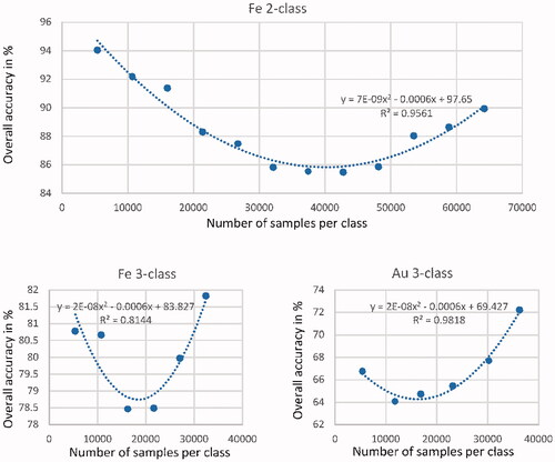
Above 30 000 samples for two classes and 18 000 samples for three classes, the accuracy results increase again, even when the lower-grade measurements are included and therefore most likely with fewer dominant correlations between grades and mineral species combinations. It is expected that the increased number of samples allows the neural network to be better trained, even if the mineral species combinations are more diverse. Again, this behaviour has been observed for iron, gold, silver and uranium. The strength of the correlation between sample numbers and overall accuracies has an R² of 0.96 (Figure 1), modelled best with a second order polynomial equation.

The results show the importance of high sample numbers for the selected machine-learning concept and that high grades can be predicted with good accuracies. This allows multiple implementation scenarios for the neural network for the prediction of geochemical assays.

Figure 2 shows the different overall accuracies of the predictions for different elements. Iron has an accuracy above 78% in the three-class approach, whereas the accuracies for gold are about 64% for the three-class approach. Two-class approaches achieve generally increased accuracies in the prediction, for iron by about 8% and for gold by about 15–18%.

Influence of knowledge of geological domains on predictions

In a subsequent evaluation step, the influence of individual geological domains on the prediction results and their accuracies was analysed. The test was performed for two different scenarios. The first scenario was characterised by comparing the results of learning on datasets from selected geological domains and comparing them against the prediction results generated for the complete Australian prediction set. In the second scenario, the neural network was trained on one geological domain, and the trained network was used for predictions on another geological domain and then compared against the complete Australian prediction set. Only drill-hole data that could clearly be allocated to the domains outlined by CSIRO, including an inverted buffer of 3 km, were incorporated. The data were then processed with similar parameters and thresholds through the neural network. The same predictor values were used for post-processing.

In a first evaluation, the training dataset was split into data from drill core from craton structures (Gawler, Yilgarn, Pilbara) and non-craton structures. Table 2 shows the results on a pairwise cross-tabulation of the prediction results (positive-class 1). The predictors were then analysed in a paired t-test. To do so, for each sample, the predictor value for the specific geo-domain was subtracted from the overall learning predictor value. For the craton dataset, the overall accuracy of the learning performance based on confusion matrices was slightly improved by up to 5%, but in the case of uranium reduced by 4%. This suggests that the neural network learning was not significantly better, even if the dataset were geologically more focused. Comparing the prediction results between the craton-only learning and the overall Australia learning, the similarities are typically above 90%, and up to 96%, except for silver with a lower level of about 87%. The predictor values correlate strongly, and the mean differences of the individual pairs of prediction are typically below 0.05 ppm. Gold has values of about 0.14 ppm higher with poorer correlations, as well as higher t-values.

Table 2. Results of the comparison of the neural network performance for geological domains (data from craton and non-cratons).

Geo-domain	Element	Threshold in ppm	n geochem class 1 (1)	Overall accuracy (2)	Overall similarity (3)	Correlation predictor (4)	Mean predictor difference (5)	SD predictor difference (6)	t value	Sig. (two-tailed)
Craton	Ag	0.5	65 830	88.02	87.00	0.83	0.02	0.19	61.00	<0.0001
	Au	0.17	31 610	83.44	96.31	0.60	0.14	0.27	270.05	<0.0001
		0.09	43 604	82.96	90.15	0.55	0.14	0.29	270.68	<0.0001
	U	0.881	28 156	85.7	94.40	0.81	0.04	0.21	97.94	<0.0001
	Cu	1150	41 742	87.54	95.63	0.81	0.02	0.19	61.42	<0.0001
Non-craton	Ag	0.5	2264	89.67	70.81	0.02	−0.09	0.43	−105.56	<0.0001
	Au	0.09	1634	94.82	77.35	0.07	0.02	0.50	23.87	<0.001
	U	0.881	4212	96.22	97.12	0.19	0.25	0.32	474.03	<0.0001
	Cu	1150	1944	93.79	90.63	0.13	−0.05	0.38	−58.69	<0.0001

Shown are the sample size used to learn (column 1), the overall accuracy achieved in the confusion matrix on the test set (column 2), the similarities on predictions using a pairwise analysis between the whole Australian dataset and the geo-domain dataset (column 3), the correlation of the predictor values (column 4), the mean of the difference of the predictor values (column 5), the standard deviation of this differences (column 6) and the parameters of the paired sample t-tests.

For the non-craton dataset, the number of learning samples was lower. The higher learning accuracy results might therefore represent the effects shown above. The prediction similarities for uranium and copper are still high, for gold and silver only 70%. In the case of higher grades of gold, the sample dataset was too small for learning, and so no results are shown. The correlations are very weak between the non-craton learned prediction and the overall Australia prediction, which has mean differences higher than in the craton dataset. Overall, it is not clear whether this is due to lower sample numbers in the dataset for learning or real differences in learning. This point indicates that using the large dataset of the whole Australia in a neural network for predicting geochemical properties has greater advantages

The learning results on separate data samples from the Yilgarn and Gawler cratons for gold and copper are shown in Table 3, with the overall learning accuracies compared. The evaluation was only performed for gold and copper because they represent larger datasets. The similarities between the predictions of the individual cratons and the overall Australian dataset are mostly above 90%. Only for lower gold grades in the Yilgarn Craton is the similarity lower with 85.7%. Correlations between the prediction results of the individual cratons and the overall Australian predictions are strong but higher in the Gawler Craton, probably owing to the larger training datasets. Mean differences between the predictions of the individual cratons and the overall Australian predictions are typically less than 0.1%, whereas they are significantly higher for gold. Summarising the results for both individual cratons, the neural network applied to individual cratons does not improve the predictions compared with the overall Australian learning model. This may be a result of the lower number of learning samples on individual cratons.

Table 3. Results of the comparison of the neural network performance for craton structures (data from Yilgarn and Gawler).

Geo-domain	Element	Threshold in ppm	n geochem class 1 (1)	Overall accuracy (2)	Overall similarity (3)	Correlation predictor (4)	Mean predictor difference (5)	SD predictor difference (6)	t value	Sig. (two-tailed)
Yilgarn	Au	0.17	8902	81.14	93.07	0.59	0.27	0.26	365.95	<0.0001
		0.09	10 278	81.30	85.74	0.55	0.30	0.27	387.32	<0.0001
	Cu	1150	2080	88.17	92.33	0.49	−0.07	0.28	−92.98	<0.0001
Gawler	Au	0.17	22 348	85.78	97.71	0.75	0.04	0.21	83.17	<0.0001
		0.09	32 838	82.68	95.21	0.74	0.03	0.22	53.32	<0.0001
	Cu	1150	39 624	83.86	94.92	0.81	0.06	0.21	123.40	<0.0001

For more details about the columns, refer to Table 2 footnote.

In a final evaluation, comparing the results of different geological domains, an experiment was set up where the sample dataset from the Gawler Craton was used to learn, and the resulting model was used for predictions in the Yilgarn Craton with no geochemical records. The predictions were again compared against the overall Australian predictions. Table 4 shows the results of the comparison for the Yilgarn Craton. The overall accuracies of the learning are only valid for the Gawler Craton, as these were learned. The similarities between the Yilgarn Craton predictions and the overall Australian predictions were mostly high, above 90%, excluding those for lower-grade gold, which were only about 83%. Correlations between predictor values of Yilgarn Craton predictions and overall Australian predictions were lower than learning on Yilgarn Craton directly (see Table 3 for gold and copper). Mean differences in the predictor values and t-values were higher for these elements. The results for silver and uranium showed higher correlations and lower t-values. In summary, learning on one craton, Gawler, and applying this model to another craton, Yilgarn, is possible, but the noise in the prediction results is larger. Overall, the results for Table 3 show more stable solutions on the predictor values when training with geochemical labels on the Yilgarn Craton to make predictions for the same craton. When analysing only the similarities on grade prediction (classification), both methods show good results. The high similarities between the Gawler Craton learned, Yilgarn Craton applied predictions and the overall Australian predictions for uranium and copper with more than 99%, which are better when learning on the Yilgarn Craton directly, are based on general geological domain differences between the cratons.

Table 4. Results of the comparison of the neural network performance for data learned on Gawler Craton and used for predictions of Yilgarn Craton data.

Geo-domain	Element	Threshold in ppm	n geochem class 1 (1)	Overall accuracy (2)	Overall similarity (3)	Correlation predictor (4)	Mean predictor difference (5)	SD predictor difference (6)	t value	Sig. (two-tailed)
Yilgarn	Ag	0.5	65 372	87.84	98.35	0.70	0.05	0.10	176.68	<0.0001
	Au	0.17	22 348	88.02	92.68	−0.02	0.52	0.34	548.73	<0.0001
		0.09	32 838	87.62	83.15	−0.05	0.52	0.33	566.37	<0.0001
	U	0.881	28 156	85.42	99.17	0.72	0.05	0.15	113.58	<0.0001
	Cu	1150	39 624	88.14	99.62	0.31	0.13	0.20	231.19	<0.0001

For more details about the columns, refer to Table 2 footnote. The overall accuracies (column 2) for the Gawler Craton, which were used for learning, are shown in bold.

Potential for resource estimation in Australia

To analyse the potential of the prediction results, a dataset of 2270 complete hyperspectral scanned drill holes, which are also available with a collar coordinate, were summarised. Column 3 of Table 5 shows the number of holes in which geochemical analysis prospectivity was established. Column 4 shows the number of holes in which the neural network predicted additional prospectivity to the existing geochemical measurements. In column 5, the table shows holes in which, without existing geochemical measurements, the neural network predicted grades above the threshold. The last column of Table 5 shows the number of holes in which 10 or more consecutive 1 m bins with grades above threshold were predicted—not having any geochemical measurement. Using the last two columns as identification of the potential of the neural network for increased deposit estimations shows that additional resources between 64% and more than 1000% can be achieved. The last column in Table 5, the increase in per cent (in parentheses) for the holes with more than 10 one-metre bins can be compared with the holes with geochemical records (sum of the columns 3 and 4). These data could improve existing exploration models. Copper and high-grade uranium have smaller increases, but especially remarkable are the improvements for nickel and bismuth.

Table 5. Exploration potential based on the predictions with the special designed neural network analysed on 2270 hyperspectral scanned drill holes.

Element	Threshold	Holes geochemical measured, but no additional prediction	Holes with geochemical measurements and additional predictions	Holes with no geochemical measurements but additional predictions	Holes with no geochemical record but 10 or more predictions (percentage of increased potential)
Ag	0.5 ppm	119	235	991	438 (124%)
Au	0.17 ppm	224	81	893	317 (104%)
	0.09 ppm	178	337	1214	616 (120%)
Fe	36.50 wt%	50	19	277	73 (106%)
	21.20 wt%	48	101	520	136 (91%)
	12.80 wt%	56	79	631	193 (143%)
	9.20 wt%	63	103	713	247 (149%)
Cu	3890 ppm	124	45	188	22 (13%)
	2000 ppm	140	75	287	52 (24%)
	1150 ppm	139	126	464	86 (32%)
U	10 ppm	98	28	81	17 (13%)
	4.27 ppm	47	117	489	80 (49%)
	0.881 ppm	25	169	956	235 (121%)
Ni	22 ppm	17	2	781	253 (1332%)
Pb	5 ppm	107	47	749	209 (136%)
Zn	68 ppm	115	36	502	93 (62%)
Sb	0.25 ppm	76	17	704	258 (277%)
As	6 ppm	17	25	954	269 (640%)
Bi	0.12 ppm	14	9	899	380 (1652%)

Shown are the number of drill holes per element and for different threshold with positive classified 1-metre bins. The geochemical measured bins are shown for comparison. The last column shows the increase in holes as a percentage compared with the holes with geochemically measured high grades for the elements.

Discussion

The evaluation shows that hyperspectral core-scan derived mineral abundances combined with sparse geochemical measurements can be used successfully with neural network methods for geological prediction. While testing the performance of the method under different conditions, the robustness of the method and importance of some key parameters have been evaluated. Regarding the input material, further evaluation of differences in hyperspectral measurements with different sensitivities and representation of the elements in the processed core scans that may influence the prediction results is needed. For the Australian core scans, which were collected over a longer time frame and processed by different operators, the authors can attest to the robustness of the data in a complex learning system. No differences between the Australian states were identified, and the predicted data were applicable for the whole Australian territory. Spectrally automatic unmixing to system scalars (i.e. sTSAS, sTSAT or sjCLST) provided a level of consistency in The Spectral Geologist software that different user scalars for the same dataset cannot. Therefore, the Australian-based public drill-core-scan system was a valuable tool for the evaluation of the influences of different parameters on an artificial intelligence system using drill-core.

While the geochemical databases provided by the Australian state geological surveys partly include information on the measurements, the authors developed the neural network under the assumption that geochemical measurements were taken under industry standards and in industry typical units. Owing to the amount of data (70 million geochemical records), in this study classical mathematical methods such as outlier and logic tests were adapted to identify critical geochemical data sets. A further assumption made was that the geochemical datasets gave a reasonable and valid representation of the corresponding depth interval allocated, as the sampled intervals from the original records are inconsistent.

Based on the results of Eichstaedt et al. (2022) on the methodological comparison of deep learning and neural network methods for the prediction of geochemical properties out of large hyperspectral drill-core archives, this article evaluates the practical implications of the specially developed neural network. The work was conducted on all elements with sufficient grade measurements in the geochemical database and includes not only gold, iron and copper but also strategically important elements such as nickel and others. Based on practical requirements, the number of classes in labelling the geochemical data was adopted. Separation based on high grades from the rest of the data or having maximum tree classes allowed better learning accuracies than more classes.

The usage of thresholds for geochemical labelling in this evaluation was still based on statistical background, but evaluating different grades for more commonly measured elements (gold, iron, copper, uranium) shows that the threshold can be adapted to strictly exploration-orientated or project-specific cutoff values. For practical applications, the neural network was able to perform predictions with high accuracies for very-high-grade segments on the drill core, even with the learning samples limited to a couple of thousand records. It must be assumed that this is based on strong correlations between hyperspectral features and high grades of the specific elements or alternative specific accompanying minerals. These effects allow the prediction of the less common base metals such as nickel, lead, antimony, bismuth and others. Here, the artificial intelligence system acts like a specialised geologist with experience in specific geological situations.

On the other hand, it was shown that with increasing numbers of learning samples, the accuracy of the prediction increases. Separating geological domains did not significantly improve the results of the prediction, and moreover the neural network with increasing numbers of learning samples was able to predict geochemical properties with good accuracies in all geological domains. The artificial intelligence systems worked here like a geologist with experience in a wide range of different projects in different regions using a vast broad knowledge. This finding indicates that the neural network trained on data from Australia can be applied to other regions globally. This will be targeted and hopefully verified by our upcoming work.

The conclusions derived open a wide range of practical applications for the developed workflow. After training on a large dataset, such as the Australian publicly available hyperspectral/geochemical databases, the system can be used on a strategic but also operational level. Scanning and hyperspectral analysis of large core collections collected by governments or private shareholders will allow a review of the geochemical potential in a short time and the allocation of new prospects in the changing world of commodities, for instance for elements used in battery production. The review could reflect changed orientation on strategic important elements and minerals supporting political decisions, economic modelling, risk evaluations and decisions on project investments. Table 5 can be used as a starting-point for such scenarios, where additionally identified drill core with nickel potential would be plotted, that might lead to geochemical samples and mineralogical zones with newly defined extensions, exploration programs reviewed, and new funding for discovery initiatives. Adding additional data into the learning data stack will improve the accuracy of the neural network prediction and the extension into potential similar neural networks for the prediction of lithological units and alteration.

The neural network can also be used in operational exploration work. Scanning core while drilling and using the predictor to identify geochemically interesting areas can free the geologist from a tedious analysis of facts that may be difficult to identify in the field and to work interactively with prediction systems on online generation of deposit models. The neural network can use the vast amounts of learning data from various geological domains with cost savings on staff, more targeted geochemical sampling and decision support during the drilling, which would outweigh the costs for core scanning with direct processing on site. Additionally, we see the application of this workflow will reduce the subjective component of interpretation and so develop a valuable tool for supporting geological staff.

Figure 3 shows the potential of the neural network on an example of drill holes in southern Australia identifying additional segments with higher uranium predictions. Using such datasets for densification of 3D modelling will allow a better understanding and growth of resources.

Figure 3. Geochemical identified higher uranium grades (above 4.5 ppm—red) and with neural network predicted additional 1 m segments with uranium contents above 4.5 ppm (green); the depth scale is on the right in metres.

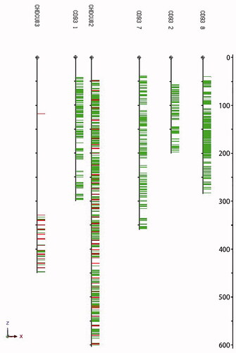
The application scenarios described above will allow drill-core data for predicted datasets such as 3D-deposit modelling and further targeting for exploration success.

Conclusions

Elemental geochemical concentrations of hundreds of kilometres of drill cores can be predicted using integrated hyperspectral drill-core scan data and limited related geochemical datasets. In this evaluation, the effects of different practical influences on the results of the prediction were tested. A specially designed convolutional-based neural network algorithm allowed predictions for geochemical properties trained on large data samples with good accuracies but also the identification of more rare elements with accuracies higher than 90%. Learning and predictions on different geological domains can be supported with large learning samples covering the whole of Australia or larger geological units such as the Gawler and Yilgarn cratons. At this stage the specially designed neural network can be used for predicting geochemical properties for the Australian region using new and existing drill core that will have commercial impact on strategic and operational exploration activities. Predicting geochemistry from hyperspectral data will allow industry to reduce costs and get a better picture of the geochemistry in drill cores. The article shows a way to identify more prospective regions or to revisit existing core under different commodity prices and requirements, as well as changed mining methods. Established technologies such as HyLogger and TSG can be used for assessment of existing and newly scanned drill core.

Acknowledgements

Authors show their gratitude towards staff members of all Australian Geological State surveys, especially Alan Mauger (SA, retired), Lena Hankock (WA), Mick Ramsey (NT), Dr Joseph Tang (Queensland), David Masters (NSW), Colin Marson (Victoria) and David Green (Tasmania). Special thanks to Dr Frederik Beuth, for his introduction and help with the implementation of the neural networks, and Joanne Ho, for preparation of parts of the material. We further thank Carsten Laukamp, for his review of the manuscript and advice for improvement.

Disclosure statement

No potential conflict of interest was reported by the author(s).

Additional information

Funding

This project was funded internally by Dimap Group and G.E.O.S. Engineering.

References

- Acosta, I. C. C., Khodadadzadeh, M., Tolosana-Delgado, R., & Gloaguen, R. (2020). Drill-core hyperspectral and geochemical data integration in a superpixel-based machine learning framework. IEEE Journal of Selected Topics in Applied Earth Observations and Remote Sensing, 13, 4214–4228. https://doi.org/10.1109/JSTARS.2020.3011221
- Arne, D. (2014). Geochemical and hyperspectral orientation study of the Redton Cu–Mo project [Technical Report for Kiska Metals Corporation]. Kiska Metals Corporation.
- AuScope. (2020). AuScope discovery portal [Online]. http://portal.auscope.org.au.
- Geoscience Australia. (2021). Australian mineral facts. Geoscience Australia. ga.gov.au.
- Bao, H. (2019). Investigations of the influences of a CNN’s receptive field on segmentation of subnuclei of bilateral amygdala. Advances in Engineering: An International Journal, 2(4), 1.
- Berman, M., Bischof, L., Lagerstrom, R., Guo, Y., Huntington, J., Mason, P., & Green, A. A. (2017). A comparison between three sparse unmixing algorithms using a large library of shortwave infrared mineral spectra. IEEE Transactions on Geoscience and Remote Sensing, 55(6), 3588–3610. https://doi.org/10.1109/TGRS.2017.2676816
- Caté, A., Perozzi, L., Gloaguen, E., & Blouin, M. (2017). Machine learning as a tool for geologists. The Leading Edge, 36(3), 215–219. https://doi.org/10.1190/tle36030215.1
- CSIRO. (2021). http://nvclwebservices.csiro.au/geoserver/wfs?&request=GetFeature&service=WFS&typename=gml:ProvinceFullExtent&outputFormat=SHAPE-ZIP&version=1.1.0
- Dramsch, J. S. (2020). 70 Years of machine learning in geoscience in review. Advances in Geophysics, 61, 1–55. https://doi.org/10.1016/bs.agph.2020.08.002
- Du, S., Wang, Y., Zhai, X., Balakrishnan, S., Salakhutdinov, R., Singh, A. (2018). How many samples are needed to estimate a convolutional Neural Network? [Paper presentation]. 32nd Conference on Neural Information Processing Systems (NeurIPS 2018), Montreal, Canada
- Eichstaedt, H., Beuth, F., Kahnt, R., & Helbig, M. (2020). Balanced applications of machine learning and geological expertise. Explorer Challenge South Australia.
- Eichstaedt, H., Ho, C. Y. J., Kutzke, A., & Kahnt, R. (2022). Performance measurements of machine learning and different neural network designs for prediction of geochemical properties based on hyperspectral core scans. Australian Journal of Earth Sciences, 69(5), 733–741. https://doi.org/10.1080/08120099.2022.2017344
- Eichstaedt, H., Tsedenbaljir, T., Kahnt, R., Denk, M., Ogen, Y., Glaesser, C., Loeser, R., Suppes, R., Alyeksandr, U., Oyunbuyan, T., & Michalski, J. (2020). Quantitative estimation of clay minerals in airborne hyperspectral data using a calibration field. Journal of Applied Remote Sensing, 14(03), 034524. https://doi.org/10.1117/1.JRS.14.034524
- Fouedjio, F., Hill, E. J., & Laukamp, C. (2018). Ore body domaining through geostatistical clustering: Case study at the Rocklea Dome Channel Iron Ore Deposit, Western Australia. Applied Earth Science, Volume 127(1), 15–29. https://doi.org/10.1080/03717453.2017.1415114
- Geng, X. (2016). Label distribution learning. IEEE Transactions on Knowledge and Data Engineering, 28(7), 1734–1748. https://doi.org/10.1109/TKDE.2016.2545658
- Green, A. (2020). CorStruth—Automated analysis of HyLogger data from the NVCL [Online]. http://www.corstruth.com.au.
- Jaques, A. L., Jaireth, S., & Walshe, J. L. (2002). Mineral systems of Australia: An overview of resources, settings and processes. Australian Journal of Earth Sciences, 49(4), 623–660. https://doi.org/10.1046/j.1440-0952.2002.00946.x
- Karpatne, A., Ebert-Uphoff, I., Ravela, S., Babaie, H. A., Kumar, V. (2020). Machine learning for the geosciences: Challenges and opportunities [Paper presentation]. 2020 IEEE Winter Conference on Applications of Computer Vision (WACV) (pp. 1765–1774).
- Kulesza, T. Amershi, S., Caruana, R., Fisher, D., Charles, D. (2014). Structured labeling to facilitate concept evolution in machine learning [Paper presentation]. Conference on Human Factors in Computing Systems—Proceedings (pp. 3075–3084).
- Lampinen, H., Laukamp, C., Occhipinti, S., & Spinks, S. C. (2016). Relationship of geochemistry and mineralogy to parent lithology and the degree of weathering in regolith [Paper presentation]. AESC 2016: Uncover Earth’s Past to Discover Our Future (p. 250).
- Leybourne, M. I., Pontual, S., & Peter, J. M. (2013). Integrating hyperspectral mineralogy, mineral chemistry, geochemistry and geological data at different scales in iron ore mineral exploration. Iron Ore Conference, 3, 10.
- Moon, C., Whateley, M., & Evans, A. (2006). Introduction to mineral exploration (2nd ed.). Blackwell.
- Neyshabur, B., Bhojanapalli, S., McAllester, D., & Srebro, N. (2017). A pac-bayesian approach to spectrally-normalized margin bounds for neural networks. arXiv preprint arXiv:1707.09564.
- O’Shea, K., & Nash, R. (2015). An introduction to convolutional neural networks. arXiv.
- Rasch, D., Herrendörfer, G., Bock, J., Victor, N. & Guiard, V. (2015). Verfahrensbibliothek: Versuchsplanung und -auswertung - Mit CD-ROM. Oldenbourg Wissenschaftsverlag. https://doi.org/10.1524/9783486843965
- Rodger, A., & Laukamp, C. (2021). Quantitative geochemical prediction from spectral measurements and its application to spatially dispersed spectral data. Applied Sciences, 12(1), 282. https://doi.org/10.3390/app12010282
- Roh, Y., Heo, G., & Whang, S. E. (2018). A survey on data collection for machine learning: A big data—AI integration perspective (p. 18). arXiv.
- Schodlok, M. C., Whitbourn, L., Huntington, J., Mason, P., Green, A., Berman, M., Coward, D., Connor, P., Wright, W., Jolivet, M., & Martinez, R. (2016). HyLogger-3, a visible to shortwave and thermal infrared reflectance spectrometer system for drill core logging: Functional description. Australian Journal of Earth Sciences, 63(8), 929–940. https://doi.org/10.1080/08120099.2016.1231133
- Sun, L., Peter, S., & Khan, S. (2019). Integrated hyperspectral and geochemical study of sediment-hosted disseminated gold at the Goldstrike District, Utah. Remote Sensing, 11(17), 1987. https://doi.org/10.3390/rs11171987