3D modelling of ground magnetic-source airborne TEM data for anisotropic media based on the rational Krylov method

Abstract

With the rapid development of the transient electromagnetic method (TEM), the numerical simulations of three-dimensional anisotropic media have garnered attention. This study used the rational Krylov method to realise the three-dimensional modelling of the ground magnetic-source airborne transient electromagnetic data for arbitrary anisotropic media. First, based on Maxwell's equations, a time-domain electromagnetic equation was derived for anisotropic media. The finite difference method was employed to discretise the equation, and the electromagnetic field was then expressed as the product of an exponential matrix and a vector related to the source. Subsequently, the rational Arnoldi algorithm was adopted to construct the rational Krylov subspace orthogonal basis vectors, and the electromagnetic fields at different times were obtained based on a model reduction strategy. The accuracy of the proposed algorithm was verified through the comparisons of its results with those of other software packages. We calculated the response for different anisotropic parameters of the typical three-dimensional anisotropic models, and analysed the influence of the anisotropic media on the ground magnetic-source airborne transient electromagnetic data. The proposed three-dimensional forward TEM algorithm provides important technical support for identifying the anisotropic geological bodies and lays the foundation for further inversion research.

KEYWORDS:

• Ground magnetic-source
• airborne
• TEM
• 3D modelling
• anisotropy
• rational Krylov method

Introduction

Compared to the ground transient electromagnetic method (TEM), the airborne TEM offers the advantages of high efficiency, low detection cost and wide exploration coverage. However, owing to restrictions on the size of the transmitting coil and current, the signal intensity transmitted by the aviation platform is weaker than that transmitted by the ground device. This results in a shallow exploration depth (Elliott 1996). In recent years, the ground-airborne TEM, also known as semi-airborne transient electromagnetic (Wu et al. 2019), has received increasing attention owing to the combination of the advantages of the high efficiency of the airborne method and the large exploration depth of the grounded method via transmission on the ground and collection in the air.

Xue et al. (2018) summarised the primary developments and important research on ground-airborne transient electromagnetic systems. Later, several review articles (Di et al. 2019, 2020; Ma et al. 2020; Lin, Xue, and Li 2021) systematically summarised the development of airborne and semi-airborne TEM from the aspects of methods, equipment, technology, and applications. The theory and application of the ground-airborne TEM first emerged in 1990s. Elliott (1996, 1998) designed the FLAIRTEM system, which uses a large loop of several kilometres as the excitation source. In test surveys conducted in various places such as Australia, the system could detect the location, inclination and depth of the mineral deposits and it successfully discovered a sulphide deposit in later applications in Indonesia. In 1997, Fugro company developed the TerraAir system that could perform full waveform continuous sampling. Smith, Annan, and McGowan (2001) used this system to collect data in Canada and found that the signal-to-noise ratio of the semi-airborne data was considerably higher than that of the airborne data. Mogi et al. (1998, 2009) designed the GREATEM system using a long wire as the excitation source and conducted a survey to investigate volcanic structures in northeastern Japan. Ito et al. (2011) used this system to reveal the underground resistivity structure in coastal areas at depth of 300–350 m up to 800 m offshore.

Excitation sources in the ground-airborne electromagnetic method can be divided into electrical and magnetic sources. Owing to the large magnetic moment of the launch device, the effective penetration depth of the electromagnetic field is greater, therefore it offers the advantages of a long detectable range and deep exploration depth (Zhang and Li 2017). This study used a large rectangular loop as the transmitter and found recent research on ground magnetic-source airborne TEM. Zhao (2013) developed a one-dimensional forward modelling algorithm for the ground loop-source airborne TEM and analysed the effects of receiving height and offset on the response. Liu (2018) used the finite difference method to realise three-dimensional forward modelling for the ground loop-source airborne TEM and simulated the response of typical models. Su (2018) applied the ground loop-source airborne method to a karst mine in Guangxi and inferred the location of a karst cave. Li, Sun, and Yang (2019) realised the three-dimensional forward modelling of the ground loop-source airborne TEM and studied the response characteristics of typical models. Yang (2020) successfully identified a water rich area of a coal mine using the ground loop-source airborne transient electromagnetic method, consequently providing geological support for safe coal mining.

Research on ground-airborne transient electromagnetic forward modelling has gradually increased in recent years; however, most studies are related to isotropic media (Witherly 2000; Ji et al. 2013; Li, Hu, and Xue 2021). Several theoretical studies and practical observations have demonstrated the widespread nature of electrical anisotropy on Earth. Because of the effect of electrical anisotropy on electromagnetic data, research on electromagnetic methods for anisotropic media has become a popular topic in electrical prospecting. Certain studies (Avdeev et al. 1998; Yin, 2004; Liu and Yin 2014; Yin et al. 2015) indicated that electromagnetic signals are sensitive to the anisotropic parameters of underground media. The use of the traditional isotropic theory to interpret transient electromagnetic data generated by anisotropic media will result in errors and even incorrect interpretation results (Yin and Maurer 2001; Weiss and Newman 2002; Yin, Qi, and Liu 2016). In terms of the technology to process ground-airborne transient electromagnetic data, the mature one-dimensional forward and inversion technologies are mainly used, and two-dimensional and three-dimensional forward and inversion methods are still under study. Few transient electromagnetic studies have considered anisotropic media, most of which focus on airborne TEM (Huang et al. 2017; Qi et al. 2020). In electrical prospecting, the incorporation of anisotropy is meaningful for establishing a model that is consistent with actual geological conditions. Moreover, it provides a new perspective for the interpretation of electrical data.

Because of the restrictions on the size of the time step, the traditional finite difference method requires thousands of iterations in time (Wang and Hohmann 1993) and solves large-scale equations many times (Namiki 1999) when used in transient electromagnetic problems. The advantage of the Krylov subspace method is that it does not require iterations in time and can directly calculate the field values at various times without solving large-scale equations (Börner, Ernst, and Güttel 2015). Druskin and Knizhnerman (1994, 1998) first introduced a rational polynomial method to solve electric fields in the time domain. Druskin, Knizhnerman, and Zaslavsky (2009) applied the rational Krylov subspace projection to solve the three-dimensional diffusion problem of the Maxwell equation, and optimised the migration parameters of the rational subspace such that the calculation results were no longer restricted by the difference in model conductivity. Börner, Ernst, and Güttel (2015) combined the rational Krylov subspace method with the finite element method to realise the three-dimensional forward modelling of TEM and proposed a new alternative optimisation method to select the pole parameters of the rational Krylov subspace. Zhou et al. (2018) proposed a single pole model reduction method in the frequency domain and used the pseudo finite volume method to achieve rapid calculation of multi-frequency three-dimensional electromagnetic problems. Qiu et al. (2020) calculated the step wave response of aviation TEM using the rational Krylov subspace method combined with the vector finite element method. Zhou et al. (2020) combined the finite volume method based on structured grids and the Krylov subspace method to obtain the full waveform three-dimensional transient electromagnetic response.

This study combined the time-domain finite difference method with the rational Krylov method to realise the three-dimensional forward modelling of ground magnetic-source airborne TEM date for arbitrary anisotropic media, and then designed a typical model to calculate and analyse the responses.

Methodology

Anisotropic conductivity

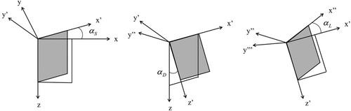
Isotropic conductivity is scalar, whereas anisotropic conductivity is a tensor. The conductivity tensor is determined using three principal conductivities ${\sigma }_x$, ${\sigma }_y$ and ${\sigma }_z$, and the three Euler rotation angles of the strike angle ${\alpha }_S$, dip angle ${\alpha }_D$ and slant angle ${\alpha }_L$. The rotational transformation adopted in this study is shown in Figure 1 (Pek and Santos 2002). It was rotated by ${\alpha }_S$ around z-axis,${\alpha }_D$ around x’-axis and ${\alpha }_L$ around z’-axis. Notably, when ${\alpha }_D$ = 0°, the rotation effect of the other two rotation angles ${\alpha }_S$ and ${\alpha }_L$ are the same; therefore the rotation angle ${\alpha }_L$ is not involved in the analysis part.

Figure 1. Transformation of the coordinate system (Pek and Santos 2002).

Let ${\sigma }^{\ast }$ be the principal conductivity tensor. It is expressed as follows: (1) ${\mathit{\sigma }}^{\ast }=\left(\begin{array}{ccc}{\sigma }_x& 0& 0\\ 0& {\sigma }_y& 0\\ 0& 0& {\sigma }_z\end{array}\right)$(1) R_x and R_z are set as the rotation matrices around the x- and z-axis, respectively, and can be expressed as follows: (2) $\begin{array}{rl}{\mathit{R}}_x(\alpha )& =\left(\begin{array}{ccc}1& 0& 0\\ 0& \cos \alpha & \sin \alpha \\ 0& -\sin \alpha & \cos \alpha \end{array}\right),\\ {\mathit{R}}_z(\alpha )& =\left(\begin{array}{ccc}\cos \alpha & \sin \alpha & 0\\ -\sin \alpha & \cos \alpha & 0\\ 0& 0& 1\end{array}\right)\end{array}$(2)

The anisotropic conductivity tensor $\stackrel{=}{\mathit{\sigma }}$ comprising nine elements, is calculated using the following formula: (3) $\begin{array}{rl}\stackrel{=}{\mathit{\sigma }}& =\left(\begin{array}{ccc}{\sigma }_{\mathrm{xx}}& {\sigma }_{\mathrm{xy}}& {\sigma }_{\mathrm{xz}}\\ {\sigma }_{\mathrm{yx}}& {\sigma }_{\mathrm{yy}}& {\sigma }_{\mathrm{yz}}\\ {\sigma }_{\mathrm{zx}}& {\sigma }_{\mathrm{zy}}& {\sigma }_{\mathrm{zz}}\end{array}\right)\\ & ={\mathit{R}}_z(-{\alpha }_S){\mathit{R}}_x(-{\alpha }_D){\mathit{R}}_z(-{\alpha }_L){\mathit{\sigma }}^{\ast }{\mathit{R}}_z({\alpha }_L){\mathit{R}}_x({\alpha }_D){\mathit{R}}_z({\alpha }_S)\end{array}$(3)

Electromagnetic equations of arbitrary anisotropic media

In this study, the finite-difference time-domain (FDTD) method was used to simulate the ground magnetic-source airborne transient electromagnetic response. Ignoring the displacement current, Maxwell’s equations in the time domain are expressed as follows (Wang and Hohmann 1993): (4) $\begin{array}{rl}-\frac{\mathrm{\partial }\mathit{b}(t)}{\mathrm{\partial }t}& =\mathrm{\nabla }\times \mathit{e}(t)\end{array}$(4) (5) $\begin{array}{rl}{\mathit{j}}_{\text{s}}(t)\text{ + }\stackrel{=}{\mathit{\sigma }}\mathit{e}(t)& =\mathrm{\nabla }\times \mathit{h}(t)\end{array}$(5) (6) $\begin{array}{rl}\mathrm{\nabla }\cdot \mathbf{b}(t)& =0\end{array}$(6) (7) $\begin{array}{rl}\mathrm{\nabla }\cdot \mathit{j}(t)& =0\end{array}$(7)

with (8) $\mathit{b}(t)=\mu \cdot \mathit{h}(t)$(8) where $\mathit{b}(t)$ is the magnetic induction intensity, ${\mathit{j}}_{\text{s}}(t)$ is the source current density, $\mathit{h}(t)$ is the magnetic field intensity, $\mathit{e}(t)$ is the electric field intensity, $\mu$ is the magnetic permeability, and $\stackrel{=}{\mathit{\sigma }}$ is the conductivity tensor.

After the turn-off time, the source current density ${\mathit{j}}_{\text{s}}(t)$ is zero, therefore, Equation 5 changes into the following form: (9) $\stackrel{=}{\mathit{\sigma }}\mathit{e}(t)=\mathrm{\nabla }\times {\mu }^{-1}\mathit{b}(t)$(9) Equations 4 and 9 are combined to eliminate the magnetic field and obtain the following equation, satisfied by the electric field: (10) $-\mathrm{\nabla }\times [{\mu }^{-1}\mathrm{\nabla }\times \mathit{e}(t)]=\overline{\overline{\sigma }}\frac{\mathrm{\partial }\mathit{e}(t)}{\mathrm{\partial }t}$(10)

Finite difference discretisation

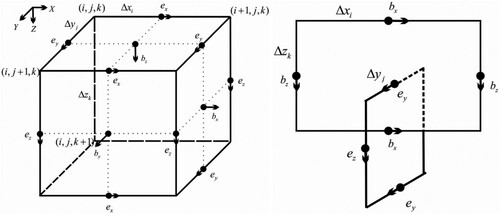
The finite difference method was used to discretise the Earth model, and a finite number of grids were used to replace the continuous space. The electric and magnetic fields were distributed in staggered grids as shown in Figure 2. Electric field was distributed at the midpoint of the edge, while magnetic field are distributed at the centre of the face. Thus, each electric field component was surrounded by four magnetic field components and each magnetic field component was surrounded by four electric field components. To balance the computing efficiency and accuracy, a non-uniform grid scheme was adopted. The core area, where the anomalous body and source were located, was divided into dense grids. In the distance, the edge length of the grid increases gradually with an expansion coefficient.

Figure 2. Staggered grid and distribution of the electromagnetic field.

To discretise Equation 10 in space, the curl operator must be considered. According to the definition of curl, the formula for calculating the curl of the electric field is as follows: (11) $\mathrm{\nabla }\times \mathit{e}=\underset{S\to 0}{lim}\left(\frac{1}{S}{\int }_c\mathit{e}\cdot d\mathit{r}\right)$(11) where c is the closed curve and S is the area surrounded by the curve. After discretisation, the curl component in the difference form is expressed as follows: (12) $\begin{array}{rl}(\mathrm{\nabla }\times \mathit{e}{)}_x& \approx e_z(i,j+1,k)/\mathrm{\Delta y}-e_z(i,j,k)/\mathrm{\Delta y}\\ & +e_y(i,j,k)/\mathrm{\Delta z}-e_y(i,j,k+1)/\mathrm{\Delta z}\end{array}$(12) (13) $\begin{array}{rl}(\mathrm{\nabla }\times \mathit{e}{)}_y& \approx e_x(i,j,k+1)/\mathrm{\Delta z}-e_x(i,j,k)/\mathrm{\Delta z}\\ & +e_z(i,j,k)/\mathrm{\Delta x}-e_z(i+1,j,k)/\mathrm{\Delta x}\end{array}$(13) (14) $\begin{array}{rl}(\mathrm{\nabla }\times \mathit{e}{)}_z& \approx e_y(i+1,j,k)/\mathrm{\Delta x}-e_y(i,j,k)/\mathrm{\Delta x}\\ & +e_x(i,j,k)/\mathrm{\Delta y}-e_x(i,j+1,k)/\mathrm{\Delta y}\end{array}$(14)

Therefore, the curl operator matrix can be expressed as curl = CR, where the matrix R contains information on the grid length, matrix C contains only $\pm 1$ and 0. The sign of the elements is dependent on the sign of each item in the above expression, and their the position in the matrix depends on the order of arrangement of the electric and magnetic fields. Further ${\mathit{M}}_{\mu }$ is the permeability matrix, which is a diagonal matrix containing the permeability of each prism and ${\mathit{M}}_{\sigma }$ is a conductivity matrix containing the conductivity tensor at each edge. In the case of arbitrary anisotropy, a transformation matrix ${\mathit{M}}_p$ carrying information regarding the change in the electric field position is also required. By multiplying the transformation matrix and the electric field vector, we can obtain the electric field components in three directions on each edge.

Using these matrices, Equation 10 can be written in matrix form: (15) $-\mathit{Ae}(t)=\mathit{B}\frac{\mathrm{\partial }\mathit{e}(t)}{\mathrm{\partial }t}$(15) where A = curl^TM_μcurl, B = M_σM_p. Mathematically, this type of equation has the following general solution, which can be expressed as the product of an exponential matrix and a vector: (16) $\mathit{e}(t)=\exp (-t{\mathit{B}}^{-1}\mathit{A}){\mathit{e}}_0$(16) where ${\mathit{e}}_0$ is the initial electric field right after the turn off time.

Initial field and boundary conditions

The magnetic induction intensity at any point in space generated by a current element can be directly calculated according to the Biot–Savart law: (17) $\mathrm{db}=\frac{{\mu }_0}{4\pi }\frac{\mathrm{Idl}\times \overrightarrow{r}}{r^3}=\frac{{\mu }_0}{4\pi }\frac{\mathrm{Idlsin}\theta }{r^2}$(17) After integration, the magnetic induction intensity generated by a finite length wire can be obtained (Gao et al. 2021): (18) $b=\frac{{\mu }_0}{4\pi }\underset{a}{\overset{b}{\int }}\frac{\mathrm{Idlsin}\theta }{r^2}$(18)

Considering each side of the transmitting loop as a finite length wire, the magnetic field generated on each side can be calculated separately and then added to obtain the initial magnetic field generated by the loop. The initial electric field can be obtained by solving Equation 9. The first type of boundary condition was adopted, which implied that the tangential electric field at the boundary was set to zero.

Rational Krylov method

The electric field expression (Equation 16), is plagued by the problem of computing the multiplication of an exponential matrix and a vector is involved. Owing to the large scale of the matrix, it is inefficient to directly calculate it using conventional computing techniques. Therefore, we used the rational Krylov subspace method to obtain an approximate solution.

The multiplication of a matrix function and a vector is generally expressed as y=f(M)r, where M is a large-scale sparse matrix, r is a vector, and f is an arbitrary function. The concept of the rational Krylov subspace method involves projecting the objective vector y into a low-dimensional Krylov subspace using a model order reduction scheme.

By projection, the approximation of the target vector y can be expressed as: (19) ${\mathit{y}}_m={\mathit{V}}_{m}f({\mathit{M}}_m){\mathit{V}}_m^T\mathit{r}$(19) where m is the order of the Krylov subspace, ${\mathit{V}}_{\text{m}}\text{ = }\{{\mathit{v}}_{\text{1}}\text{, }{\mathit{v}}_{\text{2}},\dots ,{\mathit{v}}_{\text{m}}\}$ is composed of m orthogonal basis vectors of the Krylov subspace and ${\mathit{M}}_m={\mathit{V}}_m^T\mathit{M}{\mathit{V}}_m$. The large-scale matrix can be transformed into a small or medium scale matrix, whose exponential matrix function can then be calculated directly using the function library.

In the scheme adopted herein, $\mathit{M}={\mathit{B}}^{-1}\mathit{A}$_. Further a transformation must be performed to avoid calculating the large-scale inverse matrix. First, the inner product and norm of the matrix are defined as: (20) ${⟨\mathit{x},\mathit{y}⟩}_{\mathit{B}}={\mathit{y}}^{\mathit{H}}\mathit{Bx},||{\mathit{x}}_{\mathit{B}}||=\sqrt{{⟨\mathit{x},\mathit{y}⟩}_{\mathit{B}}}$(20) where y^H denotes the conjugate transpose of y. We then use Gram-Schmidt orthogonal algorithm (Ruhe 1994) to construct the Krylov subspace K_m, and obtain the basis vector V_m of the subspace and the projection matrix A_m. The construction process is summarised in Table 1.

Table 1. Construction process of the Krylov subspace.

Construction process of Krylov subspace
01 Compute Cholesky factorisation LL^H = A–ξB
02 Set ${\mathit{v}}_{\text{1}}\text{ = }\mathit{r}\text{/}||\mathit{r}|{|}_{\mathit{B}}$
03 For j = 1, … ,m
04  Solve LL^Hw = Bvj
05  For i = 1, … ,j
06   Compute hij = <w, vi>M
w = w–vihij
07  End
08  Set $h_{j+1,j}=||\mathit{w}|{|}_{\mathit{B}}$. If $h_{j+1,j}=0$ Stop
09  Set ${\mathit{v}}_{\mathit{j}+1}=\mathit{w}/h_{j+1,j}$
10 End
11 ${\mathit{V}}_m=[{\mathit{v}}_1,{\mathit{v}}_2,\dots ,{\mathit{v}}_m]$, ${\mathit{A}}_m={\mathit{V}}_m^T\mathit{A}{\mathit{V}}_m$

For the selection of the pole $\xi$, we adopted the optimisation strategy used by Börner, Ernst, and Güttel (2015) and selected the optimal repeated pole to minimise the error in the results for the time range of 10⁻⁵–10⁻² s.

As ${\mathit{V}}_m^T\mathit{B}{\mathit{V}}_m=\mathit{I}$, Equation 16 becomes: (21) $\mathit{e}(t)={\mathit{V}}_m\exp (-t{\mathit{A}}_{\text{m}}){\mathit{V}}_m^T\mathit{B}{\mathit{e}}_0$(21)

Based on the properties of the rational Arnoldi approximation, the final formula was obtained as follows: (22) $\mathit{e}(t)={\mathit{V}}_m\exp (-t{\mathit{A}}_{\text{m}})||{\mathit{e}}_0|{|}_B{\mathit{e}}_1$(22) where ${\mathit{e}}_1=[1,0,\dots ,0{]}^T$. After obtaining the electric field at the required time, the derivative of the magnetic induction intensity with respect to the time $d{b}_z/\mathrm{dt}$ can be solved according to Equation 4. We performed a forward simulation using Fortran language based on the above theory.

Verification of the modelling accuracy

To verify the 3D forward modelling program, it’s calculation results must be compared with those of other software packages.

A set of non-uniform grids with a size of 60 × 60 × 55 was used to discretise the study area. The minimum edge length of the grid was 10 m. In the x- and y-directions, the grid was dense within a certain range from the centre. With an increase in the distance, the edge length of the grid increased gradually by an expansion factor ranging as 1.1–1.3. In the z-direction, the grid near the surface was dense and the edge length of the grid increased gradually with depth owing to the expansion factor. It extended 2200 m in the horizontal direction, 1000 m up to the air and 2500 m underground in the vertical direction. The transmitting loop adopted a step wave and unit current. We selected 31 time channels in the time range from 10⁻⁵–10⁻² s to output the results. The resistivity of the host rock for all the models in this study was set to 0.01$\text{S}\cdot {\text{m}}^{-1}$.

Response for layered isotropic model

There is a high-conductivity underground layer with a top depth of 50 m, a thickness of 100 m and a conductivity of 0.1 $\text{S}\cdot {\text{m}}^{-1}$. The size of the transmitting loop laid on the ground was 200 m × 200 m. The centre of the transmitting loop coincided with the origin of the coordinate system, and the coordinate of the receiver in the air was (0, 0, −30 m). The results were consistent with those of the AarhusInv software (Auken et al. 2015) developed by Aarhus University in Denmark, as shown in Figure 3; an error of less than 2.8% was observed. We also used the time-domain second-order implicit backward Euler method to calculated the results using the direct solver Pardiso. Through our testing, we found that the new method was more efficient when the calculation accuracy met the requirements. In this example, we used the same computer, and the new method took 435.3 s while the traditional implicit backward Euler method took 524.7 s. A comparison is shown in Figure 4 and the results are in good agreement, with an error of less than 2.7%

Figure 3. Comparison with results of AarhusInv software.

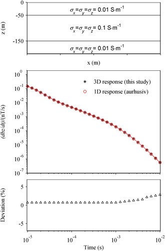
Figure 4. Comparison with results of implicit backward method.

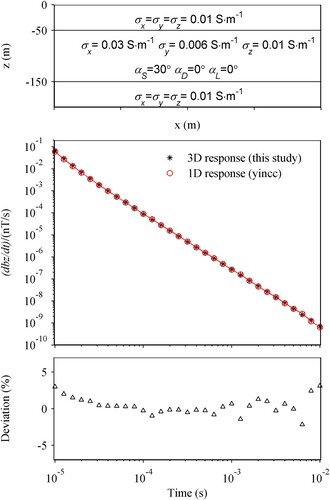
Response for layered arbitrary anisotropic model

An arbitrary anisotropic layer was placed underground with a top depth of 50 m, and thickness of 100 m. The three principal conductivities were ${\sigma }_x$ = 0.03$\text{S}\cdot {\text{m}}^{-1}$, ${\sigma }_y$ = 0.006$\text{S}\cdot {\text{m}}^{-1}$, and ${\sigma }_z$ = 0.01$\text{S}\cdot {\text{m}}^{-1}$. Further, the three rotation angles were ${\alpha }_S$ = 30°, ${\alpha }_D$ = 0°, and ${\alpha }_L$ = 0°. The size of the transmitting loop was 20 m × 20 m. The transmitting loop was laid on the ground and the receiver was located at the centre of the loop. The results were compared with those obtained using Yin Changchun's one-dimensional arbitrary anisotropic transient electromagnetic modelling software (Yin and Weidelt 1999). As shown in Figure 5, the results were in good agreement, with an error of less than 3.2%.

Figure 5. Comparison with the results of one-dimensional anisotropy software.

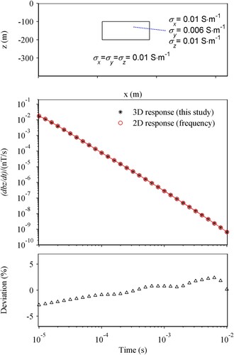
Response for two-dimensional principal anisotropic model

A two-dimensional prism underground extending infinitely in the y-direction was oberved. The depth of the top was 100 m, the size in the x-direction was 200 m, and the size in the z-direction was 100 m. The three principal conductivities ${\sigma }_x$, ${\sigma }_y$, and ${\sigma }_z$ of the prism were set to 0.01, 0.006 and 0.01$\text{S}\cdot {\text{m}}^{-1}$ respectively. An in-loop device was adopted, and the transmitting loop was located on the ground, with dimensions of 20 m × 20 m. The receiver was located at the centre of the transmitting loop. Compared with the results of the two-dimensional anisotropic transient electromagnetic forward modelling program (Guan 2019) based on the finite element method, as shown in Figure 6, the results were in good agreement with an error of less than 2.9%.

Figure 6. Comparison with the results of two-dimensional anisotropic software.

By comparing the response of the isotropic layered model, arbitrary anisotropic layered model and two-dimensional principal anisotropic model with other software, we have verified the calculation accuracy of three-dimensional arbitrary anisotropy ground magnetic-source airborne transient electromagnetic method forward algorithm.

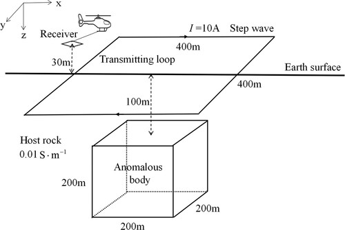
Three-dimensional model

We simulated the response of a typical three-dimensional anisotropic model to analyse the influence of different anisotropic parameters on the ground magnetic-source airborne transient electromagnetic response. We designed an anomalous body with a top depth of 100 m, and its length, width, and height all set to 200 m. A transmitting loop of size 400 m × 400 m was laid on the ground and located at (0, 0, 0). The amplitude of the transmitted current was 10 A, and the waveform was a step wave. The receivers were located in air at a height of 30 m and the survey area covered 800 m × 800 m. Here, 21 measuring lines were designed, each containing 21 measurement points. Therefore, the number of measuring points was 441, and the distances between points and lines were 20 m. The other device and grid discretisation parameters were identical to those described in the previous verification section. Figure 7 shows a schematic of the 3D model.

Figure 7. Sketch of 3D model.

Two cases were considered to determine the location of the anomalous body. In the first case, an anomalous body was located immediately below the transmitting loop. The centre of the anomalous body’s projection onto the surface coincided with the centre of the transmitting loop. In the second case, the position of the anomalous body was shifted by 200 m in the x-direction. Thus, the anomalous body’s projection on the surface was at (200 m, 0, 0). We choose a regular cube as the anomalous body to eliminate the response characteristics caused by different structural scales in three directions. This allowed us to focus on studying the influence of the anisotropic parameters of the anomalous body.

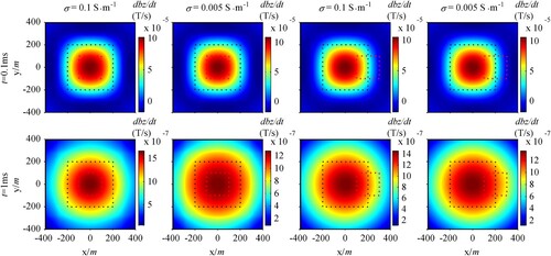
Response for isotropic media

For comparison, we require a basic understanding of the ground magnetic-source airborne transient electromagnetic response for isotropic media. ${\sigma }_0$ is the conductivity of the host rock, which was uniformly set to 0.01$\text{S}\cdot {\text{m}}^{-1}$.${\sigma }_{}$ is the conductivity of the anomalous body and was set to 0.1 and 0.005$\text{S}\cdot {\text{m}}^{-1}$. As shown in Figure 8, we selected two time channels, t = 0.1 and 1 ms, to show the response. The black dotted line box represents the position of the transmitting loop, and the red dotted line box represents the projection of the anomalous body on the surface. The original response had a circular shape and gradually diffused over time. However, reflecting the influence of the resistivity parameters of the 3D abnormal bodies from the original response was challenging. Therefore, we used the method of subtracting the response of homogeneous half-space with conductivity of 0.01 $\text{S}\cdot {\text{m}}^{-1}$ from the original response and analysed the remaining anomalous response.

Figure 8. Original response for isotropic anomalous body.

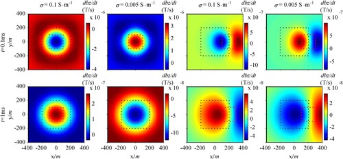
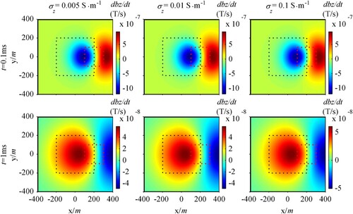
Anomalous responses are shown in Figure 9. We consider the response at 0.1 ms. When the anomalous body was immediately below the transmitting loop, the anomalous response exhibited an extrema above the anomalous body. If the conductivity of the anomalous body was higher than that of the host rock, the extrema was the minimum, otherwise, it was a maximum. When the position of the anomalous body shifted in the x-direction, two extreme points appeared on both sides of the anomalous body along the x-direction. If the conductivity of the anomalous body was higher than that of the host rock, the extremum close to the loop was a minimum, and that far from the loop was a maximum. Otherwise, the opposite was true. At 1 ms, the response diffused, and the sign of the extremum was reversed.

Figure 9. Anomalous response for isotropic anomalous body.

Response for arbitrary anisotropic media

Effect of horizontal conductivity ${\sigma }_x$

The vertical conductivity ${\sigma }_z$ and horizontal conductivity ${\sigma }_y$ of the anomalous body were both set to be 0.02$\text{S}\cdot {\text{m}}^{-1}$. The other horizontal conductivity ${\sigma }_x$ was set to be 0.005$\text{S}\cdot {\text{m}}^{-1}$, 0.01$\text{S}\cdot {\text{m}}^{-1}$, and 0.1$\text{S}\cdot {\text{m}}^{-1}$ respectively. Geological conditions corresponding to this anisotropic model exist in nature. Vertical joints may appear in rocks under stress and certain sedimentary rocks or schists can form vertical rock layers owing to tectonic movements. In these cases, the anisotropic conductivity of the rocks satisfies ${\sigma }_x$<${\sigma }_y$ = ${\sigma }_z$. If the metamorphic rock is composed of columnar minerals, it also exhibits electrical anisotropy, resulting in ${\sigma }_x$>${\sigma }_y$ = ${\sigma }_z$.

Figure 10 shows the anomalous response for different conductivity ${\sigma }_x$ when the anomalous body is immediately below the transmitting loop. First, we consider the response at 0.1 ms. When ${\sigma }_x$ was lower than ${\sigma }_0$, the anomalous response exhibited two symmetrical maximums on both sides of the anomalous body along the x-direction and two symmetrical minimums along the y-direction. When ${\sigma }_x$ was equal to ${\sigma }_0$, the two minimums along the y-direction were combined into one, which was immediately above the anomalous body. When ${\sigma }_x$ was higher than ${\sigma }_0$, there were two symmetrical maximums on both sides of the anomalous body along y-direction and a minimum right above the anomalous body along the x direction. When t = 1 ms, the anomalous response diffused, however, the sign of the extremums reversed.

Figure 10. Anomalous response for different ${\sigma }_x$ when anomalous body is immediately below the transmitting loop.

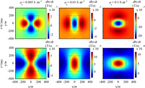
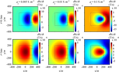
Figure 11 shows the anomalous response for different conductivities in ${\sigma }_x$ when the position of the anomalous body is shifted. When t = 0.01 ms, despite the different ${\sigma }_x$, all anomalous responses displayed two extremums on both sides of the anomalous body along the x-direction. The extremum close to the loop was the minimum and the extremum far from the loop was the maximum. When ${\sigma }_x$ was higher than ${\sigma }_0$, the anomalous response was distorted along the x-direction. At t = 1 ms, the anomalous response diffuses over time; however the sign of the extremums was reversed.

Figure 11. Anomalous response for different ${\sigma }_x$ when the position of the anomalous body is shifted.

Effect of horizontal conductivity ${\sigma }_y$

The vertical conductivity ${\sigma }_z$ and horizontal conductivity ${\sigma }_x$ of the anomalous body were both set to be 0.02$\text{S}\cdot {\text{m}}^{-1}$. The other horizontal conductivity ${\sigma }_y$ was set to be 0.005$\text{S}\cdot {\text{m}}^{-1}$, 0.01$\text{S}\cdot {\text{m}}^{-1}$, and 0.1$\text{S}\cdot {\text{m}}^{-1}$ respectively. The geological body corresponding to this anisotropic model was similar to that described in the previous section, except for the change in direction.

Figure 12 shows the anomalous response for different conductivity ${\sigma }_y$ when the anomalous body is immediately below the transmitting loop. According to the symmetry, it was similar to the anomalous response when ${\sigma }_x$ acquired different values as that in the previous section; however, the characteristics in the x- and y-directions were interchanged.

Figure 12. Anomalous response for different ${\sigma }_y$ when anomalous body is immediately below the transmitting loop.

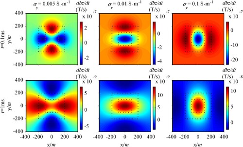
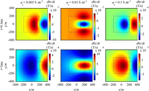
Figure 13 shows the anomalous response for different conductivity ${\sigma }_x$ values when the position of the anomalous body was shifted. First, we focus on the anomalous response at 0.01 ms. When ${\sigma }_y$ was lower or higher than ${\sigma }_0$, the anomalous responses exhibited two extremums on both sides of the anomalous body along the x-direction. The difference was that when ${\sigma }_y$ was lower than ${\sigma }_0$, the extremum close to the loop was a maximum and that far from the loop was a minimum. The opposite was ture when ${\sigma }_y$ was greater than ${\sigma }_0$. When ${\sigma }_y$ was equal to ${\sigma }_0$, the anomalous response generated two maximums along the y-direction and a minimum along the x-direction. At t = 1 ms, the anomalous response diffused; however, the sign of the extremums reversed.

Figure 13. Anomalous response for different ${\sigma }_y$ when the position of the anomalous body is shifted.

Effect of vertical conductivity ${\sigma }_z$

The horizontal conductivities ${\sigma }_x$ and ${\sigma }_y$ of the anomalous body were both set to be 0.02$\text{S}\cdot {\text{m}}^{-1}$. The vertical conductivity ${\sigma }_z$ was set to 0.005, 0.01, and 0.1$\text{S}\cdot {\text{m}}^{-1}$. Geological conditions corresponding to this anisotropic model are common in nature. For example, most sedimentary and foliated metamorphic rocks have layered structures that result in ${\sigma }_z$<${\sigma }_x$ = ${\sigma }_y$. If the metamorphic rock has a columnar structure, its anisotropic conductivity satisfies ${\sigma }_z$>${\sigma }_x$ = ${\sigma }_y$.

As shown in Figures 14 and 15, the change in ${\sigma }_z$ had minimal effect on the anomalous response. The anomalous response was primarily affected by the conductivity in the horizontal direction. As the conductivity along the horizontal direction was greater than that of the surrounding rock, the response characteristics were similar to those in the previous section, where the conductivity of the isotropic anomalous body was higher than that of the surrounding rock.

Figure 14. Anomalous response for different ${\sigma }_z$ when anomalous body is immediately below the transmitting loop.

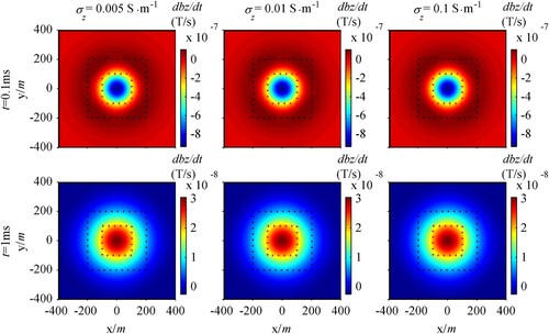
Figure 15. Anomalous response for different ${\sigma }_z$ when the position of the anomalous body is shifted.

Effect of strike angle ${\alpha }_S$

The three principal conductivities of the anomalous body were set as ${\sigma }_x$ = 0.02$\text{S}\cdot {\text{m}}^{-1}$, ${\sigma }_y$ = 0.005$\text{S}\cdot {\text{m}}^{-1}$ and ${\sigma }_z$ = 0.02$\text{S}\cdot {\text{m}}^{-1}$. The rotation angles were set as ${\alpha }_D$ = ${\alpha }_L$ = 0°and ${\alpha }_S$ = 0°, 30°, 60°, and 90°. This indicates that the anomalous body rotated horizontally around the z-axis during tectonic movement and the direction of the three principal conductivities did not completely coincide with the coordinate axis.

Figure 16 shows the anomalous responses for different ${\alpha }_S$ when the anomalous body was located immediately below the transmitting loop. When ${\alpha }_S$ acquired different values, the horizontal conductivity axis and the coordinate axes did not always coincide. At t = 0.1 ms, the anomalous response displayed two symmetrical minimums along the direction of high conductivity and two symmetrical maximums along the direction of low conductivity. The line connecting the two maximums or the two minimums is the symmetry axis of the response, which rotated at the angle of ${\alpha }_S$ in the horizontal plane. The anomalous response gradually diffused over time, and the sign of the extremums was reversed.

Figure 16. Anomalous response for different ${\alpha }_S$ when anomalous body is immediately below the transmitting loop.

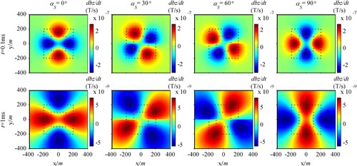
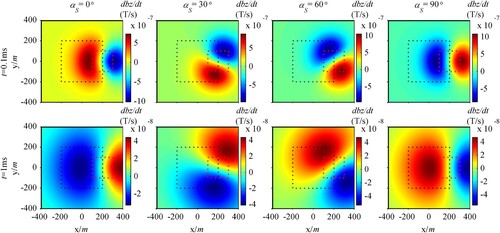
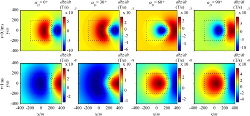
Figure 17 shows the anomalous response for different conductivity ${\alpha }_S$ when the position of the anomalous body is shifted. When ${\alpha }_S$ = 0°, the situation was the same as that presented in Figures 12 and 13 when ${\sigma }_y$ was lower than ${\sigma }_0$. With ${\alpha }_S$ acquiring different values, the response rotated in horizontal plane at the angle of 2${\alpha }_S$. When t = 1 ms, the anomalous response diffused and the sign of the extremums reversed.

Figure 17. Anomalous response for different ${\alpha }_S$ when the position of the anomalous body is shifted.

Effect of dip angle ${\alpha }_D$

The three principal conductivities of the anomalous body were set as ${\sigma }_x$ = 0.02$\text{S}\cdot {\text{m}}^{-1}$, ${\sigma }_y$ = 0.005$\text{S}\cdot {\text{m}}^{-1}$ and ${\sigma }_z$ = 0.02$\text{S}\cdot {\text{m}}^{-1}$. The rotation angle was ${\alpha }_S$ =${\alpha }_L$ = 0°, and ${\alpha }_D$ = 0°, 30°, 60°, and 90°. This indicated that the anomalous body rotated horizontally around the z-axis during tectonic movement and the direction of the three principal conductivities did not completely coincide with the coordinate axis.

Figure 18 shows the anomalous responses for different ${\alpha }_D$ when the anomalous body was located immediately below the transmitting loop. When ${\alpha }_D$ = 0°, the situation was the same as in the previous section when ${\sigma }_y$ was lower than ${\sigma }_0$. With an increase in ${\alpha }_D$, the two extremums along the x-direction gradually approached, forming one extremum immediately above the anomalous body, and the two extremums along the y-direction gradually faded away. When ${\alpha }_D$ increased to 90°, the conductivity in the y-direction was equal to that in x-direction; therefore, the electromagnetic field diffused at the same speed in horizontal direction and the anomalous response formed a circle.

Figure 18. Anomalous response for different ${\alpha }_D$ when anomalous body is immediately below the transmitting loop.

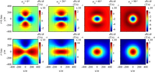
Figure 19 shows the anomalous response for different ${\alpha }_D$ when the position of the anomalous body was shifted. When ${\alpha }_D$ = 0°, the situation was also the same as that in the previous section when ${\sigma }_y$ was lower than ${\sigma }_0$. The angle ${\alpha }_D$ implies rotation around the x-axis. When it acquires different values, the conductivity and coordinate axes do not coincide completely. The conductivity in the y-direction resulted from the interaction between ${\sigma }_y$ and ${\sigma }_z$. With an increase in ${\alpha }_D$, the effect of ${\sigma }_z$ increased. When the conductivity in the y-direction exceeded that of the host rock and continued to increase, the sign of the extremums was reversed. When ${\alpha }_D$ increased to 90°, the conductivity in the y-direction became ${\sigma }_z$, which was equal to ${\sigma }_x$ and higher than ${\sigma }_0$. Therefore, the response characteristics were similar to those in the pevious section, where the isotropic anomalous body had high conductivity.

Figure 19. Anomalous response for different ${\alpha }_D$ when the position of the anomalous body is shifted.

The effects of the various anisotropic parameters on the response differed. At the end of this section, we provide a brief summary and comparison of the main effects in Table 2.

Table 2. The influence of various anisotropic parameters on the response.

	Parameters
	Horizontal	Horizontal	Vertical
Anomalous	conductivity	conductivity	conductivity	Strike angle	Dip angle
position	${\sigma }_x$	${\sigma }_y$	${\sigma }_z$	${\alpha }_S$	${\alpha }_D$
Right below the transmitting loop	1. Positions of the extremums are interchanged 2. Response is stretched		${\sigma }_z$ almost has no influence on the response	The responses rotates ${\alpha }_S$ degrees in the horizontal plane and its shape remains unchanged	Response is stretched
Shifted in x-direction	Response is stretched				1. Positions of the extremums are interchanged 2. Response is distorted
	Response is distorted	Positions of the extremums are interchanged

Conclusions

Based on the finite difference and rational Krylov methods, this study proposed a 3D forward algorithm of the ground magnetic-source airborne TEM for arbitary anisotropic media. The advantages of the Krylov subspace method are that it does not require iterations in time, avoids solving large-scale equations, and can efficiently calculate the field values at different times. We calculated the anomalous response for typical anisotropic theoretical models and analysed the influence of the anisotropic parameters on the ground magnetic-source airborne transient electromagnetic response. As evident, the ground magnetic-source airborne transient electromagnetic response for anisotropic media is obviously different from that for isotropic media. The combination of different anisotropic parameters resulted in more complex response characteristics. The horizontal principal conductivity had a significant effect on the response, whereas the vertical principal conductivity had minimal effect. The effect of all the rotation angles on the response cannot be ignored. Our research provides technical support for identifying underground anisotropic geological bodies from ground magnetic-source airborne transient electromagnetic data and lays the foundation for future inversion work.

Acknowledgements

This work was supported by the High performance Computing Platform of China University of Geosciences Beijing.

Disclosure statement

No potential conflict of interest was reported by the author(s).

Additional information

Funding

This study was supported by the National Natural Science Foundation of China [Nos. 41830429].

References

- Auken, E., A.V. Christiansen, C. Kirkegaard, G. Fiandaca, C. Schamper, A.A. Behroozmand, A. Binley, E. Nielsen, F. Effersø, and N.B. Christensen. 2015. An overview of a highly versatile forward and stable inverse algorithm for airborne, ground-based and borehole electromagnetic and electric data. Exploration Geophysics 46: 223–35. doi:10.1071/EG13097.
- Avdeev, D.B., A.V. Kuvshinov, O.V. Pankratov, and G.A. Newman. 1998. Three-dimensional frequency-domain modeling of airborne electromagnetic responses. Exploration Geophysics 29: 111–9. doi:10.1071/EG998111.
- Börner, R.-U., O.G. Ernst, and S. Güttel. 2015. Three-dimensional transient electromagnetic modelling using rational Krylov methods. Geophysical Journal International 202: 2025–43. doi:10.1093/gji/ggv224.
- Di, Q., G. Xue, C. Yin, and X. Li. 2020. New methods of controlled-source electromagnetic detection in China. Science China: Earth Sciences 63, no. 9: 1268–77.
- Di, Q., R. Zhu, G. Xue, C. Yin, and X. Li. 2019. New development of the electromagnetic (EM) methods for deep exploration. Chinese Journal of Geophysics 62, no. 6: 2128–38. CNKI:SUN:DQWX.0.2019-06-012.
- Druskin, V., and L. Knizhnerman. 1994. On application of the Lanczos method to solution of some partial differential equations. Journal of Computational and Applied Mathematics 50: 255–62. doi:10.1016/0377-0427(94)90305-0.
- Druskin, V., and L. Knizhnerman. 1998. Extended Krylov subspaces: Approximation of the matrix square root and related functions. SIAM Journal on Matrix Analysis and Applications 19: 755–71. doi:10.1137/S0895479895292400.
- Druskin, V., L. Knizhnerman, and M. Zaslavsky. 2009. Solution of large scale evolutionary problems using rational Krylov subspaces with optimized shifts. SIAM Journal on Scientific Computing 31: 3760–80. doi:10.1137/080742403.
- Elliott, P. 1996. New airborne electromagnetic method provides fast deep-target data turnaround. The Leading Edge 15, no. 4: 309–10. doi:10.1190/1.1437333.
- Elliott, P. 1998. The principles and practice of FLAIRTEM. Exploration Geophysics 29, no. 2: 58–60. doi:10.1071/eg998058.
- Gao, J., M. Smirnov, M. Smirnova, and G. Egbert. 2021. 3-D time-domain electromagnetic modeling based on multi-resolution grid with application to geomagnetically induced currents. Physics of the Earth and Planetary Interiors 312: 106651. doi:10.1016/j.pepi.2021.106651.
- Guan, Q.C. 2019. 2.5 dimensional modeling of transient electromagnetic data for anisotropic media. Beijing: China University of Geosciences. doi:10.27493/dcnki.gzdzy.2019.001748.
- Huang, W., F. Ben, C.-C. Yin, Q.-M. Meng, W.-J. Li, G.-X. Liao, S. Wu, and Y.-Z. Xi. 2017. Three-dimensional arbitrarily anisotropic modeling for time-domain airborne electromagnetic surveys. Applied Geophysics 14: 431–40. doi:10.1007/s11770-017-0627-8.
- Ito, H., T. Mogi, A. Jomori, Y. Yuuki, K. Kiho, H. Kaieda, K. Suzuki, K. Tsukuda, and S.A. Allah. 2011. Further investigations of underground resistivity structures in coastal areas using grounded-source airborne electromagnetics. Earth, Planets and Space 63: e9–e12. doi:10.5047/eps.2011.08.003.
- Ji, Y., Y. Wang, J. Xu, F. Zhou, S.Y. Li, Y. Zhao, and J. Lin. 2013. Development and application of the grounded long wire source airborne electromagnetic exploration system based on an unmanned airship. Chinese Journal of Geophysics 56: 3640–50. doi:10.6038/cjg20131105.
- Li, X., W. Hu, and G. Xue. 2021. 3D modeling of multi-radiation source semi-airborne transient electromagnetic response. Chinese Journal of Geophysics 64, no. 2: 716–23. doi:10.6038/cjg2021O0166.
- Li, Y., H. Sun, and J. Yang. 2019. Three-dimensional modeling of semi-airborne transient electromagnetic with loop source. Journal of China Coal Society 44, no. S2: 631–42. doi:10.13225/j.cnki.jccs.2018.1628.
- Lin, J., G. Xue, and X. Li. 2021. Technological innovation of semi-airborne electromagnetic detection method. Chinese Journal of Geophysics 64, no. 9: 2995–3004. doi:10.6038/cjg2021P0409.
- Liu, K. 2018. Numerical simulation of the finite difference of transient electromagnetic field in the rectangular loop of air-ground system. Xi’an: Chang’an University. CNKI:CDMD:2.1018.792364.
- Liu, Y., and C. Yin. 2014. 3D anisotropic modeling for airborne EM systems using finite-difference method. Journal of Applied Geophysics 109: 186–94. doi:10.1016/j.jappgeo.2014.07.003.
- Ma, Z., Q. Di, D. Lei, Y. Gao, J. Zhu, and G. Xue. 2020. The optimal survey area of the semi-airborne TEM method. Journal of Applied Geophysics 172: 103884. doi:10.1016/j.jappgeo.2019.103884.
- Mogi, T., K. Kusunoki, and H. Kaieda. 2009. Grounded electrical-source airborne transient electromagnetic (GREATEM) survey of mount Bandai, north-eastern Japan. Exploration Geophysics 40: 1–7. doi:10.1071/eg08115.
- Mogi, T., Y. Tanaka, K. Kusunoki, T. Morikawa, and N. Jomori. 1998. Development of grounded electrical source airborne transient EM (GREATEM). Exploration Geophysics 29, no. 2: 61–4. doi:10.1071/eg998061.
- Namiki, T. 1999. A new FDTD algorithm based on alternating-direction implicit method. IEEE Transactions on Microwave Theory and Techniques 47, no. 10: 2003–7. doi:10.1109/22.795075.
- Pek, J., and F.A. Santos. 2002. Magnetotelluric impedances and parametric sensitivities for 1-D anisotropic layered media. Computers & Geosciences 28: 939–50. doi:10.1016/S0098-3004(02)00014-6.
- Qi, Y., X. Li, C. Yin, Z. Qi, J. Zhou, N. Sun, Y. Liu, and B. Zhang. 2020. Three-dimensional adaptive finite-element method for time-domain airborne EM over an anisotropic earth. Chinese Journal of Geophysics 63: 2434–48. doi:10.1016/j.jappgeo.2016.05.013.
- Qiu, C., C. Yin, Y. Liu, B. Zhang, X. Ren, Y. Qi, and J. Cai. 2020. 3D time-domain airborne electromagnetic forward modeling using the rational Krylov method. Chinese Journal of Geophysics 63: 715–25. doi:10.6038/cjg2020M0494.
- Ruhe, A. 1994. The rational Krylov algorithm for nonsymmetric eigenvalue problems. III: Complex shifts for real matrices. BIT Numerical Mathematics 34: 165–76. doi:10.1007/BF01935024.
- Smith, R.S., A.P. Annan, and P.D. McGowan. 2001. A comparison of data from airborne, semi-airborne and ground electromagnetic systems. Geophysics 66, no. 5: 1379–85. doi:10.1190/1.1487084.
- Su, C. 2018. Response and experimental studies of semi-airborne transient electromagnetic for shallow karst. Jinan: Shandong Univesity. doi:10.7666/d.Y3411337.
- Wang, T., and G.W. Hohmann. 1993. A finite-difference, time-domain solution for three-dimensional electromagnetic modeling. Geophysics 58: 797–809. doi:10.1190/1.1889155.
- Weiss, C.J., and G.A. Newman. 2002. Electromagnetic induction in a fully 3-D anisotropic earth. Geophysics 67: 1104–14. doi:10.1190/1.1500371.
- Witherly, K. 2000. The quest for the Holy Grail in mining geophysics: A review of the development and application of airborne EM systems over the last 50 years. The Leading Edge 19: 270–4. doi:10.1190/1.1438586.
- Wu, X., G.Y. Fang, G.Q. Xue, L.H. Liu, L.S. Liu, and J.T. Li. 2019. The development and applications of the helicopter-borne transient electromagnetic system CAS-HTEM. Journal of Environmental & Engineering Geophysics 24, no. 4: 653–63. doi:10.2113/jeeg24.4.653.
- Xue, G.Q., X. Li, S.B. Yu, W.Y. Chen, and Y.J. Ji. 2018. The application of ground-airborne TEM systems for underground cavity detection in China. Journal of Environmental and Engineering Geophysics 23, no. 1: 103–13. doi:10.2113/JEEG23.1.103.
- Yang, P.Q. 2020. Research on 3D Forward Modeling and Application of Ground to Air Transient Electromagnetic Field. Energy and Environmental Protection 42, no. 8: 131–135. doi:10.19389/j.cnki.1003-0506.2020.08.028.
- Yin, C. 2004. The effect of electrical anisotropy on the response of airborne electromagnetic systems. Seg Technical Program Expanded Abstracts 20: 1169–76. doi:10.1190/1.1816401.
- Yin, C., and H.-M. Maurer. 2001. Electromagnetic induction in a layered earth with arbitrary anisotropy. Geophysics 66: 1405–16. doi:10.1190/1.1487086.
- Yin, C., Y. Qi, and Y. Liu. 2016. 3D time-domain airborne EM modeling for an arbitrarily anisotropic earth. Journal of Applied Geophysics 131: 163–78. doi:10.1016/j.jappgeo.2016.05.013.
- Yin, C., and P. Weidelt. 1999. Geoelectrical fields in a layered earth with arbitrary anisotropy. Geophysics 64: 426–34. doi:10.1190/1.1444547.
- Yin, C.C., B. Zhang, Y.H. Liu, X.Y. Ren, and J. Cai. 2015. Review on airborne EM technology and developments. Chinese Journal of Geophysics – Chinese Edition 58: 2637–53. doi:10.6038/cjg20150804.
- Zhang, Y.Y., and X. Li. 2017. Research progress on ground-airborne transient electromagnetic method. Progress in Geophysics 32, no. 4: 1735–41 (in Chinese). doi:10.6038/pg20170443.
- Zhao, Y. 2013. Multi-component study of air-ground transient electromagnetic method system. Xi’an: Chang’an University. doi:10.7666/d.D407496.
- Zhou, J., W. Liu, X. Li, Y. Qi, and Z. Qi. 2020. 3-D full-time TEM modeling using shift-and-invert Krylov subspace method. IEEE Transactions on Geoscience and Remote Sensing 58: 7096–104. doi:10.1109/TGRS.2020.2979798.
- Zhou, J., W. Liu, H. Liu, X. Li, and Z. Qi. 2018. Research on rational Krylov subspace model order reduction algorithm for three-dimensional multi-frequency CSEM modelling. Chinese Journal of Geophysics 61, no. 6: 2525–2536. doi:10.6038/cjg2018L0311.