Which glaucoma patients benefit from 10-2 visual field testing? Proposing the functional vulnerability zone framework

ABSTRACT

Clinical relevance

A method for determining 10-2 deployment in glaucoma with the goal of detecting additional visual field sensitivity for the purpose of functional monitoring is proposed.

Background

To provide a pilot method for determining when to deploy the 10-2 visual field (VF) test grid in glaucoma by characterising the ‘functional vulnerability zone’.

Methods

The cross-sectional 24-2 (central 12 locations) and 10-2 VF results from 133 eyes of 133 glaucoma subjects were used to describe the central Hill of Vision using VF sensitivity. The ‘volume’ (defined using arbitrary units, A.U.) under the Hill was calculated. A greater A.U. on the 10-2 indicated a functional vulnerability zone (FVZ), signifying additional clinical dynamic range for potential future monitoring. The main outcome measures were calculated A.U. and 24-2 factors which were significantly related to A.U. differences between 24-2 and 10-2.

Results

Over 55% of patients had an FVZ (A.U. greater using 10-2). Several 24-2 features (worse mean deviation, worse central 24-2 mean defect, and a higher proportion of defective locations) were significant in the FVZ cohort compared to non-FVZ. 24-2 mean deviation levels at which 10-2 may be favoured were low at −3.16 to −3.62 dB. Specifically, 5 or more defective central 24-2 test locations were associated with an FVZ. Subjects exhibiting a less severe defect on the 10-2 were more likely to have an FVZ, indicating its potential for future VF monitoring.

Conclusions

The authors propose several clinical markers, focussing on the 24-2, which can guide clinicians on when the 10-2 may have utility in glaucoma assessment. The authors provide a pilot reference spreadsheet for clinicians to visualise the likelihood of 10-2 utility in the context of an FVZ.

KEYWORDS:

• 10-2
• 24-2
• central visual field
• Humphrey Field Analyzer
• macula visual fields
• perimetry

Introduction

Modern patient management paradigms in glaucoma aim to prevent irreversible blindness and to preserve quality of life, and both goals are measured largely through the visual field component of glaucoma testing.^1–3 Currently, the clinical standard is white-on-white static automated perimetry that measures increment thresholds at various locations across the visual field.⁴ Through a combination of practical experience and historical precedent,⁵ the 24-2 has become a widely used test grid as it covers locations that are typically affected in glaucoma,⁶ as well as offering a practical number of test locations useful in clinical practice.⁷ For example, a SITA-Faster 24-2 test can assess 52 test locations covering a visual field extent approximately 24 degrees from fixation plus two nasal points in approximately 2-3 minutes.^8,9

Recently, several groups have highlighted the importance of focussing on visual field testing within the central visual field (such as 10 degrees from fixation), due to the impact of centrally located defects on activities of daily living and quality of life.^10–12 Central visual field defects are also important in current glaucoma staging systems as their presence typically escalate the severity of the disease to its more advanced stages.^2,13 A higher prevalence of central visual field defects identified using the 10-2 have been reported in some studies,^14,15 but others have suggested that the detection of central visual field defects is similar in commonly used glaucoma-related visual field test grids, 24-2, 24-2C and 10-2.^16–21

Aside from defect detection, progression analysis is an important factor in glaucoma assessment. Recent groups have suggested that the 10-2 may provide additional information for progression analysis in some patients when using a global index, mean deviation.^22,23 This has been cited to be largely attributable to the lower variability of results returned by the 10-2 grid. However, aside from the global score, the potential additive value of the 10-2 may be its ability to monitor the characteristic pattern of deepening and widening of centrally located scotomata over time in glaucoma with more numerous and closer spaced test locations.

Historical examples of the so-called deepening and widening of glaucomatous scotomata were visualised using kinetic perimetry by examining the closeness of isopters by demonstrating the boundary of the scotoma and its effect on the Hill of Vision.^24–26 However, the boundary is less well defined when using conventional, sparse clinical test grids in static perimetry. High-density, condensed static automated perimetry test grids have highlighted the characteristic deepening and widening of the scotoma, but these do not necessarily represent a practical approach to clinical testing.²⁷ Aside from the question related to detection or characterisation of central visual field loss, there is limited guidance on utility with respect to dynamic range for the purposes of obtaining meaningful data. For example, even if both test grids demonstrate a hemifield loss, there is no obvious quantitative strategy for determining which returns more clinically useful information. Thus, there is interest in determining the potential value of denser test grids used to assess the central visual field, such as the 10-2, compared to the standard 24-2 grid, and whether that affords benefits in terms of dynamic range with different glaucomatous defects.³

Clinically, there are two broad scenarios for 10-2 deployment: 1) detection or confirmation of a defect, and 2) expanding opportunities to identify residual visual field sensitivity for ongoing disease monitoring. The authors refer to the latter scenario where the 10-2 affords dynamic range benefits (i.e. extending beyond the floor of the 24-2 through increased spatial sampling) as the presence of a ‘functional vulnerability zone’, and this was the focus of the present investigation.

In the present study, the authors tested the hypothesis that a quantitative method for comparing dynamic range can be elicited, where some patients have a clinical benefit in 10-2 testing because of the ability to characterise residual dynamic range (functional vulnerability zone present), whilst other patients have no such benefit (functional vulnerability zone absent). The end goal was to propose a pilot model or framework upon which future empirical data can be applied.

Methods

This study was a retrospective pilot study. Ethics approval for the study was provided by the Human Research Ethics Committee of the University of New South Wales (HC210563). The study adhered to the tenets of the Declaration of Helsinki. Subjects provided written informed consent prior to inclusion in the study.

Subject data, inclusion, and exclusion criteria

Subjects in the study consisted of patients attending the optometry-ophthalmology collaborative care glaucoma service at the Centre for Eye Health, University of New South Wales.^28–30 The study cohort (meeting the inclusion criteria described below) was extracted from the cohort of patients with glaucoma that were seen consecutively between January and June 2021 to reduce the potential for spectrum bias. The diagnosis of glaucoma was made as per current clinical guidelines² and as per the criteria described in the authors’ previous studies.^20,21 In brief, glaucomatous structural defects included enlarged or asymmetric cup-to-disc ratio, diffuse or focal rim thinning, and adjacent retinal nerve fibre layer defects that were not explained by other retinal or neurological pathologies. For the purposes of the present study, the subjects were required to have a visual field defect found on static automated perimetry that was concordant with the structural defect (patients with pre-perimetric glaucoma were excluded). As per the protocols of the clinic, all patients with an initially noted or suspected central visual field defect on the 24-2 (or 24-2C) test grid (defined as at least one location of the 12 within the central 10 degrees with a probability score was p < 0.01 of lower) and/or had glaucomatous structural defects found on a macular (ganglion cell-inner plexiform layer thickness) scan subsequently underwent testing using a 10–2 test grid. Whilst a more liberal criteria could have been adopted (such as testing all patients with both grids irrespective of what defect they may have demonstrated), this sampling strategy reflects a clinical paradigm in which a 10–2 is performed in the context of suspected centrally involved field (on the 24-2) or structural (on optical coherence tomography) loss (see discussion). Testing was performed on the same day. The data were sourced from an existing database and thus included newly-diagnosed patients and those already on treatment.

For inclusion in the study, the subject with glaucoma must have had 10-2 (SITA-Fast) and 24-2 (SITA-Faster) visual field data performed on the Humphrey Field Analyzer (HFA3, Carl Zeiss Meditec, Dublin, CA), and the results must have met the manufacturer’s reliability criteria, as described in the authors’ previous work (<15% false positives, no seeding point errors, and <20% of occasions with gaze tracker deviations exceeding 6 degrees).^31,32 Subjects who had 24-2C (SITA-Faster) data were included, but the additional central 10 test locations were not included for analysis. As these test points within the 24-2C test grid are assessed at the end of the test, their inclusion was unlikely to affect the other visual field sensitivity results, and the FORUM software also provides 24-2 mean deviation data. As the goal was to develop a model that could identify differences in clinical outputs using a real-world approach, the authors did not further modulate the output sensitivity results from the different SITA algorithms (see below). Importantly, visual field test results are known to be fluctuant. The goal of the present study was to perform a head-to-head comparison of 24-2 and 10-2 results on the same day, which is why confirmation of a defect was not explicitly required, reflecting a practical clinical situation. In other words, the purpose of this framework was not to obtain multiple results to conclusively determine the repeatability using the same test grid.

Exclusion criteria included: age <18 years, visual acuities worse than 6/9, history of ocular trauma or surgery (but included those who had undergone uncomplicated cataract surgery, selective laser trabeculoplasty, or laser peripheral iridotomy), and the presence of macular, retinal, or neurological pathology that may affect the visual field measurement. Patients with dense cataracts that impacted the integrity of the visual field, as identified by comparing the consistency and pattern of total and pattern deviation maps, were excluded from the study.

Definition of glaucomatous visual field defects

All subjects had statistically significant reductions in visual field sensitivity as detected on the pattern deviation map on both the 10-2 and 24-2 test grids. Typical criteria for determining the significance of visual field loss require a combination of statistically significantly reduced sensitivity values that are contiguous. Due to the limited number of test locations assessed within the central visual field on the 24-2 test grid, contiguity for the defects seen on the 24-2 was not required. Instead, the study used a criterion of a compounded probability score of at least p < 0.001 across the central test locations (for example, at least one point reduced at a probability level of p < 0.001, or at least two contiguous points reduced at a level of p < 0.01 each).^20,33 The 10–2 uses different probability levels (it does not report p < 0.001 probability scores). The same compounded probability score cut-off was used for significance, and thus at minimum it required two contiguous points reduced at a level of p < 0.01 each.

Visual field data extraction

Visual field data (24-2 and 10-2) sensitivity results, probability scores, and global indices were extracted using a custom written program on MATLAB (MathWorks, Natick, MA). In addition, the subject’s age, self-reported gender, self-reported ethnicity, and spherical equivalent refractive error were extracted directly from their electronic medical health record.

All pointwise results from the 10-2 were used in the subsequent analysis (68 total test locations). Only the central 12 test locations within a 10-degree radius from fixation of the 24-2 were included to compare similar test areas within the central 10 degrees.

Analysis of visual field sensitivity

The pilot framework focussed on output sensitivity values (dB) from both test grids. Alternative measures included total deviation and pattern deviation. Sensitivity was chosen for this study as total deviation and pattern deviation values rely on the underlying normative database. Furthermore, although sensitivity outputs are affected by the thresholding algorithm (such as SITA-Faster or SITA-Fast), the total deviation and pattern deviation values are further derivatives of sensitivity values and are thus affected by further confounding factors. Despite differences in algorithms and normative databases, the use of unmodulated sensitivity results reflects the goal of leveraging currently available clinical data.

The functional vulnerability zone model: description

The authors describe the proposed framework as the functional vulnerability zone (FVZ), which represents a zone of visual field that is assessed on the 10-2 (or indeed any other denser test grid) but not the 24-2. The concept of ‘vulnerability’ reflects the proposal of seeking test locations that reveal additional perimetric information, i.e. unaffected or less affected sensitivities. This notably differs from prior studies examining solely detection rates, which recognise to be another useful aspect of 10-2 deployment, as the outcome of interest in this proposed framework reflects clinically useful information in the form of dynamic range, as described below. Notably, this also differs from the ‘macular vulnerability zone’ coined by Hood and colleagues, which describes a region of the macula proposed to have higher frequencies of structural loss.³⁴ The aspect of ‘vulnerability’ described by the framework refers specifically to regions at-risk of further functional loss adjacent to an existing defect identified by visual field testing.

The authors propose three potential FVZ outcomes, illustrated in the schematic in Figure 1A. For simplicity of visualisation, Figure 1A depicts hypothetical scenarios in which there is a ‘core’ defect identified using both visual field test grids (represented by the blue X), and a region of relative normality along a particular visual field test meridian. Normative data from the authors’ previous publication³⁵ is depicted as a yellow shaded region for reference.

Figure 1. Schematic of the models developed in the present study. In A: the Functional Vulnerability Zone (FVZ) concept is shown using a two dimensional representation of sensitivity (y-axis) as a function of test location (x-axis). The outcomes are dependent on the relative relationship between sensitivities obtained using the 24-2 (red) and 10-2 (black), relative to a normative distribution from the authors’ previous publication (yellow zone), as described in the text. The FVZ is highlighted using the orange bars in outcome 3 (right panel). In B: 24-2 (red crosses) and 10-2 (blue circles) for a representative patient are shown for visual field sensitivity as a function of test location (x and y locations).

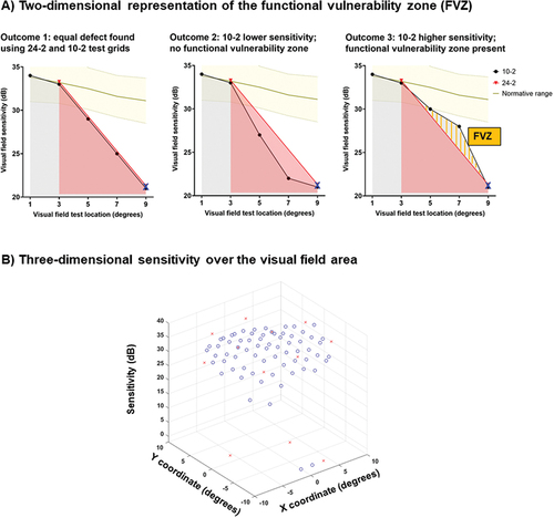
• Outcome 1: Both 24-2 and 10-2 defects are identical, i.e. there is no FVZ.

• Outcome 2: The 10-2 provides no additional information, as the defect at locations between equivalent 24-2 test locations are deep. Even if a 10-2 was conducted, the depth of the additional defect (well below the normative range) would not be expected to add significant information for measuring residual visual function more so than the 24-2. Thus, there is also no FVZ.

• Outcome 3: The 10-2 provides additional information, as the 10-2 test locations between 24-2 test locations have a sensitivity result higher than the predicted slope between normal and defect. These test locations represent the region of the theoretical FVZ (orange bars), using which clinical information related to disease progression can still be elicited in future (i.e. additional remnant dynamic range).

As illustrated in Figure 1A, the utility of the 10-2 in providing additional information to the clinician is dependent on the desired outcome or aim of comparing its outcomes with the 24-2. In outcomes 1 and 2, the 10-2 could still be deployed to confirm the presence of a visual field defect detected using a 24-2. This has been previously studied and is thus not the focus of this paper.

However, if the clinician aims to detect test locations that offer different information that expands the dynamic range relative to 24-2 results, outcome 3, where a FVZ is identified, would be desired. Clinically the FVZ can translate into visual field regions that can potentially be a) leveraged for monitoring progression and b) a target to be ‘saved’ from future sensitivity loss. Thus, outcome 3, which was denoted as the presence of an FVZ, was the focus of this investigation.

Calculating the functional vulnerability zone (FVZ)

To identify the FVZ, 3-dimensional plots of the measured sensitivity values for the 10-2 and 24-2 test grids were created, analogous to visualisation of the Hill of Vision. The x- and y-coordinates represented the test locations in the visual field, and the z-axis represented the visual field sensitivity (Figure 1B).

Then, the ‘volume’ under the Hill of Vision was determined by integrating (using the trapezoidal rule) the z-axis along the x- and y-axes. Because sensitivity was used for the Hill of Vision, this meant that the integration was performed from the top down towards 0 dB, similar to the shading indicated by Figure 1A. Given that sensitivity is reported as an instrument-specific quantity (in this case, from the Humphrey Field Analyzer), instead of reporting the integral as a true volume (such as dB/deg²), this was reported in arbitrary units (A.U.). The method of reporting A.U. therefore makes no assumption about magnitudes of significance (especially given that dB is itself not a linear unit), but rather focuses on identifying trends favouring one or the other test grid in terms of the residual instrument-measured sensitivity within that part of the visual field. This is effectively represented by the following equation.

$\mathit{A}.\mathit{U}.={\int }_{-9}^9{\int }_{-9}^9\mathit{z}\mathit{dx}\mathit{dy}$

Where the limits of integration were −9 to 9, representing the area spanned by the region of interest within the test grids.

The null hypothesis was that there is no difference in A.U. between the 24-2 and the 10-2. A higher A.U. found using the 10-2 compared to the 24-2 would indicate the presence of an FVZ where there is residual visual field sensitivity. Conversely, a lower A.U. found using the 10-2 compared to the 24-2 indicates no FVZ, and thus limited utility of the 10-2. In other words, here, the volumetric calculation is a numerical representation of the geometry of the measured visual field.

Describing clinically meaningful transitions in perimetric sensitivity

The superimposition of 10-2 and 24-2 using the model described in Figure 1 allowed us to infer which test grid might have more opportunities for detecting sensitivity change. However, it has been well documented that there is a heteroskedastic relationship between the test-retest variability and underlying visual field sensitivity, with low sensitivity values being associated with greater variability.^36,37 Because of the variability, the amount of change that needs to occur to be deemed significant is larger at lower sensitivity values as glaucoma progresses. In other words, the fact that sensitivity differences at various levels have different significance need to be considered, where granular changes in small decibel steps may still be within test-retest variability. Thus, although sensitivity outputs may be reported in 1 dB steps, a ‘step of meaningful change’ is more likely to span a wider range of decibel values.

An additional analysis using pre-defined sensitivity steps was performed and this is further described in the Supplementary Material.

Statistical analysis

Subjects were grouped into whether they had an FVZ (favouring the 10-2 test grid) or no evidence of an FVZ (non-FVZ group, favouring the 24-2 test grid), recalling that the favourability refers specifically to dynamic range and not defect detection.

The perimetry variables of interest were as follows: 24-2 mean deviation, 10-2 mean deviation, difference in mean deviation, average 24-2 central sensitivity (calculated using total deviation results of the 12 central 24-2 test locations), proportion of defects (p < 0.05) within the 12 test locations of the 24-2, proportion of defects within the 10-2, difference in proportion of defects and difference in number of defects. These were compared between FVZ and non-FVZ groups using Wilcoxon rank sum test. Linear regression analyses were performed on differences in A.U. calculations between 10-2 and 24-2 and the variables listed above to identify factors that might explain whether a patient has an FVZ or no FVZ. Then, binary logistic regression and principal components analyses^38,39 (the latter considers and acknowledges that some variables may be correlated) were used to account for variables that were correlated with each other to determine a final model that might predict whether a patient would likely have an FVZ.

The binary logistic regression and principal components analyses were performed firstly with both 10-2 and 24-2 parameters (as the purpose was to determine whether a given 10-2 result would, in comparison, offer a greater dynamic range with a paired 24-2 result), and secondly with only 24-2 parameters (in the context where there needs to be a decision regarding whether to perform a 10-2 if only given a 24-2 result).

A p-value of less than 0.05 was considered statistically significant. Statistical analyses were performed on GraphPad Prism version 8 (La Jolla, CA) and SPSS version 26 (IBM Statistics).

Results

The characteristics of the 133 subjects included in the present study are shown in Table 1. Most subjects had an early stage of glaucoma according to their mean deviation, but as per the inclusion criteria, all had significant central visual field defects, and the mean deviation results overall, spanned the full dynamic range of the Humphrey Field Analyzer (+1.05 to −29.84 dB).

Table 1. Demographic and clinical characteristics of the 133 subjects examined in the present study.

Parameter
Age (years) median, IQR, full range		64.7, IQR 55.3–72.7, full range 28.1–88.9
Self-reported gender (n, %)	Male	71 (53.4%)
	Female	62 (46.6%)
Self-reported ethnicity (n, %)	Caucasian	50 (37.6%)
	East Asian	72 (54.1%)
	South Asian	10 (7.5%)
Eye (n, %)	Right eye	70 (52.6%)
	Left eye	63 (47.4%)
Humphrey Field Analyzer 24-2 indices	Mean deviation (dB) median, IQR	−4.08, IQR −6.83 to −2.34
	Pattern standard deviation (dB) median, IQR	5.50, IQR 2.96 to 8.31
Humphrey Field Analyzer 10-2 indices	Mean deviation (dB) median, IQR	−3.11, IQR −5.85 to −1.72
	Pattern standard deviation (dB) median, IQR	3.34, IQR 1.89 to 8.33
Cirrus optical coherence tomography results	Average retinal nerve fibre layer thickness (microns) median, IQR	72.5, IQR 63.8 to 80.0
	Average ganglion cell-inner plexiform layer thickness (microns) median, IQR	68.0, IQR 62.0 to 73.0
Spherical equivalent refractive error (dioptres) median, IQR		−0.25, IQR −3.50 to +1.00

IQR = interquartile range.

‘Volume’ of the Hill of Vision

The A.U. measurements, indicating the remaining ‘volume’ of the Hill of Vision, for the 24-2 and 10-2 test grids are shown in Figure 2. There were significant differences when considering the A.U. measurements when using sensitivity outputs (Figure 2A, p = 0.0404), with the 10-2 having a higher A.U. compared to the 24-2.

Figure 2. Arbitrary units (A.U.) measurements for sensitivity outputs expressed as a pairwise comparison (A) and a difference plot (B) for 24-2 and 10-2 test grids. In B) a positive y-axis value indicates that the 24-2 had a higher A.U. measurement (grey shaded area), and a negative y-axis value indicates that the 10-2 had a higher A.U. measurement (blue shaded area). Each datum point indicates the result from one subject, and the box and whiskers indicate the median, interquartile range and full range. The asterisk indicates a p < 0.05 and ns indicates no significant difference.

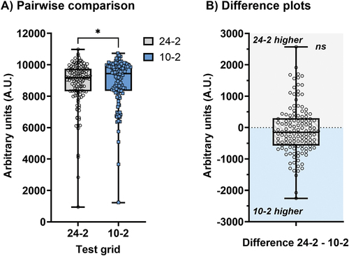
However, there was also substantial overlap in the A.U. results. Thus, when examining individual subjects and their outcomes, with 80/133 (60.2%) having a higher A.U. on the 10-2 compared to the 24-2, thus the presence of a potential FVZ. A one sample t-test showed no significant difference when using sensitivity (p = 0.2044), suggesting heterogeneity amongst the cohort (Figure 2B). Notably, this highlights a core concept that a subset of patients would benefit from 10-2 testing (FVA present) for the purposes of dynamic range, but this would not apply to all patients. For the ensuing analyses, subjects with an A.U. favouring the 10-2 was identified as the ‘FVZ’ group, and an A.U. favouring the 24-2 as the ‘non-FVZ’ group (i.e. whichever test grid returned the absolute higher A.U. value).

Factors contributing to the difference between FVZ and non-FVZ groups

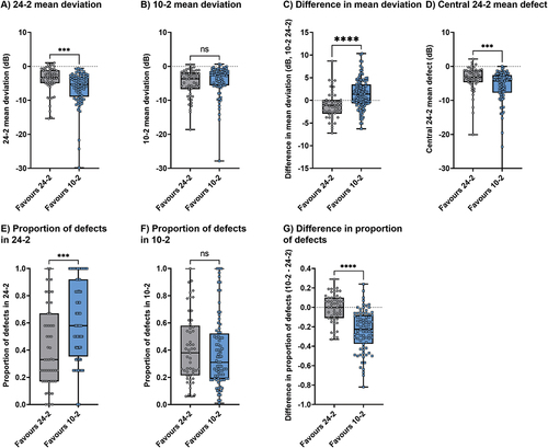
The authors considered several factors that might have contributed to the differences between the FVZ and non-FVZ groups. For the grouping determined by the A.U. found using sensitivity measurements, 24-2 mean deviation was significantly lower (p = 0.0002, mean difference −2.03 dB), central 24-2 mean defect was significantly lower (p = 0.0006, mean difference −1.12 dB), the proportion of 24-2 defects was significantly higher (p = 0.0001, mean difference 0.25) and difference in proportion of defects between test grids was significantly lower (p < 0.0001, mean difference −0.23) for the FVZ group (favouring the 10-2). Although the 10-2 mean deviation was not significantly different between groups, the difference in mean deviation between 10-2 and 24-2 was significantly different (p < 0.0001, by 2.45 dB). These results are shown in Figure 3.

Figure 3. Differences between the FVZ (favouring 10-2) and non-FVZ (favouring 24-2) groups across variables of interest when using sensitivity measurements to calculate A.U. The asterisks indicate statistically significant differences (***, p < 0.001; ****, p < 0.0001) and ns indicates no significant difference.

Regression analysis of difference in A.U. as a function of variables of interest

Regression analyses when considering the difference in A.U. calculated using sensitivity outputs are shown in Figure 4. All variables of interest except the proportion of defects found on the 10-2 showed a significant slope. However, the highest coefficient of determination was found when the regression analysis was performed as a function of difference in mean deviation (R² = 0.5440), followed by the difference in proportion of defects (R² = 0.3246) with all other variables each accounting for less than 10% of variance. The x-intercepts, which represent the transition between favouring the 10-2 and the 24-2, are also shown in Figure 4. When examining the factor with the highest coefficient of determination, a positive difference in A.U. favouring the 10-2 was associated with a difference in mean deviation of x > 0.46 dB (i.e. 10-2 more positive compared to the 24-2). When considering the difference in proportion of defective locations, a positive difference in A.U. favouring the 10-2 was associated with a difference in proportion of defective locations of x <  −0.08 (i.e. that the 10-2 had a lower proportion of defects compared to the 24-2).

Figure 4. Regression analyses of the difference in A.U. (10-2 – 24-2, calculated using sensitivity) as a function of variables of interest in the present study. Each datum point represents one patient. A positive y-axis value indicates a result favouring the 10-2 (FVZ present), and a negative y-axis value indicates a result favouring the 24-2 (FVZ absent). The p-value and R² are shown in the inset. The red vertical arrow indicates the x-intercept for each regression line.

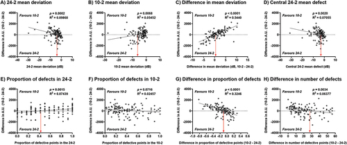
Regression analyses performed with the 24-2 mean deviation results in Figure 4 suggested that a linear regression might not be the optimal fitting method. This might be expected because as mean deviation worsens over time, eventually neither perimetric test pattern would offer useful clinical information, thus the difference in A.U. between 10-2 and 24-2 would expectedly approach 0. Therefore, the fit of data was also examined using a quadratic equation instead. The coefficients of determination were marginally improved when using quadratic regression. When considering the A.U. calculations using sensitivity, the first x-intercepts were −3.62 dB and −3.16 dB for 24-2 mean deviation and central 24-2 mean defect, respectively, similar to that shown in Figure 5 (Supplementary Figure S4).

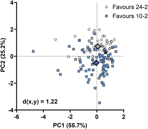
Figure 5. Biplot showing principal components (PC) 1 and 2 following principal components analysis. Each datum point indicates the result from one patient, grouped into whether an FVZ was present (favouring 10-2, blue squares) or absent (favouring 24-2, white circles), based on sensitivity A.U. calculations. The large diamonds represent the ‘average’ for FVZ and non-FVZ groups, and the Euclidean distance (d(x,y)) between them is shown in the lower left.

Binary logistic regression and principal components analysis

Then, whether an FVZ was absent or present was binarised. Binary logistic regression analysis was performed to identify factors that might predict the outcome. The results of the binary logistic regression analysis are shown in Table 2. When using the A.U. calculations obtained using sensitivity measurements, the difference in mean deviation (p < 0.0001) and difference in proportion of defective locations (p < 0.0001) were found to be significant in the regression model (Nagelkerke R² = 0.514). Results for the analysis performed using sensitivity brackets are shown in Supplementary Table S1.

Table 2. Binary logistic regression analysis outcomes using the forward stepwise method.

	Unstandardised B	Unstandardised standard deviation	p-value
Difference in mean deviation	0.33	0.89	<0.0001
Difference in proportion of defective locations	−5.386	1.341	<0.0001

Since the variables of interest were potentially correlated (albeit at different magnitudes), principal components analysis was also performed to determine aggregate factors (principal components) that encompassed correlated variables that could then create a Z-score predicting the outcome of whether an FVZ is likely present or absent. The results of the principal components analysis are shown in Table 3 and Figure 5. Principal components 1 and 2 accounted for 80.9% of the total variance. The biplots showing the data points converted into Z-scores along principal components 1 and 2 show a distinct separation of subjects with an FVZ (favouring the 10-2, blue squares) and those without (favouring the 24-2, white circles). Thus, a patient with a score that is more negative along principal components 1 (i.e. a worse 24-2 and 10-2 mean deviation, a worse central 24-2 mean defect, and more visual field defects on the 24-2 and 10-2) and 2 (i.e. a lower mean deviation on the 24-2 compared to the 10-2, more visual field defects on the 24-2, and fewer defects on the 10-2 compared to the 24-2) is more likely to have an FVZ. The Euclidean distances between the ‘average’ FVZ and non-FVZ patient was 1.22 when calculating A.U. using sensitivity (results for sensitivity brackets are shown in Supplementary Figure S5).

Table 3. Rotated component matrix the principal components analysis.

	PC1 (55.7%)	PC2 (25.2%)
24-2 mean deviation	0.847
10-2 mean deviation	0.931
Difference in mean deviation		−0.845
Central 24-2 mean defect	0.912
Proportion of defective locations in 24-2	−0.748	−0.469
Proportion of defective locations in 10-2	−0.869
Difference in proportion of defective locations		0.851

A simplified predictor of 10-2 utility using only 24-2 parameters

The regression and principal components analysis above were conducted using both 10-2 and 24-2 test parameters to examine a situation where both results are available, but there needs to be a quantitative indicator for dynamic range given a pair of results. However, there may be situations in which a clinician may wish to decide based solely on a 24-2 result.

Binary logistic regression analysis with only the 24-2 test parameters as variables was performed, and found that only the proportion (or number) of central 24-2 defects (out of 12) was significantly (A.U. calculated using sensitivity: unstandardised B = 1.275, SD = 0.317, p < 0.0001; A.U. calculated using sensitivity brackets or steps: unstandardised B = 1.136, SD = 0.309, p < 0.0001) related to the presence or absence of the FVZ. The Nagelkerke R² was lower (A.U. calculated using sensitivity, R² = 0.173; A.U. calculated using sensitivity brackets or steps, R² = 0.143) than when 10-2 parameters were also considered, which reflected the smaller number of potentially explanatory variables.

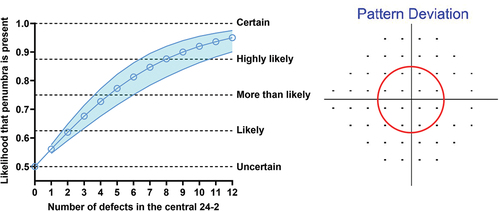
Since only one parameter was found to be significant, principal components analysis was not subsequently performed as it would not be meaningful. Instead, the regression result was used to calculate the likelihood that an FVZ is present, shown in Figure 6. The likelihood spans from 0.5 to 1, where the lower limit of 0.5 indicates uncertainty (50–50 that an FVZ would be present, and no better than guessing) and the upper limit of 1 indicates certainty (the asymptote at which a 10-2 is certainly beneficial). Additional qualitative levels are shown for illustrative purposes. As expected, an increasing number of 24-2 defects leads to a greater likelihood that an FVZ will be revealed by the 10-2.

Figure 6. Likelihood that an FVZ is present (y-axis) as a function of number of centrally affected test locations (at the p < 0.05 level or lower) on the pattern deviation map of the 24-2 test grid (x-axis; the region of interest is shown by the red circle on the right hand panel). At each number of defects, the blue open circle indicates the likelihood, with the shaded region indicating the variance of the estimated likelihood (1 standard deviation). The horizontal dashed lines indicate qualitative impressions of certainty spanning from the lower limit of the y-axis 0.5 (uncertain − 50–50 chance), 0.625 (likely), 0.75 (more than likely), 0.875 (highly likely) to 1.0 (certainty, which represents an asymptote).

Discussion

In the present pilot study, the authors developed a model to determine when a 10-2 visual field test grid may offer useful additional clinical information to the 24-2 test grid when assessing patients with glaucoma, which is an enduring question in the field. The authors used an approach where the Hill of Vision was examined using a ‘volumetric’ approach, allowing a description of the presence or absence of a FVZ, which would imply that the 10-2 has greater residual sensitivity or dynamic range.

The key results are summarised as follows. First, not all subjects appeared to have an FVZ, and in such cases, the 10-2 test grid theoretically adds little additional useful information specifically with respect to dynamic range. Second, features within the 24-2 test grid result (worse mean deviation, worse central 24-2 mean defect, and a higher proportion of defective locations) were found in the cohort with an FVZ. Accordingly, subjects in whom the 10-2 had a more positive (less severe) mean deviation and had proportionally fewer defects compared to the 24-2 were more likely to have an FVZ. Whilst a 24-2 mean deviation or central 24-2 mean defect of −3.16 to −3.62 dB or −2.32 to −2.71 dB appeared to be a cut-off for the onset of 10-2 usefulness, the strongest relationship remained the proportion of defects found centrally (0.41, or 5 or more, of the 24-2 test locations). Given these parameters, the authors have also devised two simple aids: first, a pilot-data derived downloadable spreadsheet to aid the clinician in deciding upon deployment of the 10-2 based on the likelihood of an FVZ being present (described further below); and second, a simplified predictor of whether an FVZ is likely to be present given the number of centrally affected 24-2 test locations (Figure 6).

Describing the FVZ in visual fields: lessons from stroke

The core premise of this paper is to illustrate the usefulness of additional test locations for expanding the dynamic range of visual field testing, and not just for defect detection. The increased resolution of the 10-2 visual field test grid compared to the 24-2 grid for defining the FVZ draws parallels with the concept of measuring the ischaemic penumbra in stroke, whereby useful information can be discerned by analysing two superimposed regions of interest.

The ischaemic penumbra is a zone the surrounds the core of a brain infarct, and was first described over 40 years ago as a region of hypoperfusion within thresholds of functional impairment and structural integrity, which has the capacity for recovery with reperfusion.⁴⁰ In the present model, the FVZ in visual field testing reflects a potential zone where residual visual field sensitivity or test dynamic range, if captured, allows for ongoing monitoring of the glaucomatous visual field defect. Thus, analogous to stroke, it represents an area where there is the possibility of a measurable and preservable visual field in future. In clinical practice, this is therefore represented by higher test density grids, such as the 10-2.

However, by virtue of the number of central test locations present in the 10-2, there are naturally more test locations at which a defect could be detected, i.e. 68 test locations on the 10-2 versus 12 within the 24-2, and thus a one-to-one comparison of the absolute number of sensitivity brackets or steps with the 24-2 would not be fair. A simple count would also fail to acknowledge the pattern of visual field defect, i.e. how it is deepening or widening, as per the conventional description of glaucomatous defects.^27,41

Thus, a method was used to account for the test density. Using a ‘volumetric’ approach analysing the Hill of Vision, the authors interpolated across test locations to estimate the residual visual field sensitivity or remaining sensitivity brackets or steps. This concept resembles that of kinetic perimetry or static campimetry, as it identifies deviations in the profile of the Hill of Vision,⁴² thus providing an estimate of the volume of the Hill of Vision. There are inherent limitations of interpolating and integrating across test locations, especially when the distance between test locations is relatively large, as demonstrated by Westcott and colleagues.⁴³ The authors did not aim to obtain fine resolution and ‘smoothed’ visual field maps like Westcott and colleagues,⁴³ as the goal was to examine the utility of currently available clinical test grids.

In essence, the FVZ model also infers the edge or border of the scotoma, or its ‘gradient’. Aoyama and colleagues⁴⁴ used a similar interpolation method when adding additional test locations between existing 24-2 test locations to quantify the border of the scotoma. They described differences between scotomata with ‘flat’ and ‘steep’ gradients initially described by the 24-2, whereby ‘steep’ gradients are more likely to benefit from customised, additional intervening test locations to fully understand the scotomata. The FVZ model is consistent with their previous findings and adds to this by using a global approach to understand if the 10-2 would be additive, without customising the test. Overall, the results emphasise the need to characterise the glaucomatous visual field defect.

Each perimetry device returns a sensitivity value that is dependent on its maximum luminance output and background luminance level, and it is reported in logarithmic (decibel) units reflecting the attenuation of maximum test luminance.⁵ Thus, a volume quantity (dB/deg²), such as Aoyama and colleagues,⁴⁴ was not used, but instead the authors chose to use arbitrary units (A.U.). This unit mainly served as a comparison between test grids, rather than as a precise measurement of visual field sensitivity. Alternative methods to both dB/deg² and A.U. included percentage remaining and deviation/deg². However, percentage remaining would likely return a result similar to A.U., and deviation/deg² has a similar problem with being instrument specific due to its normative comparisons.

Factors affecting the visual field FVZ

The present study specifically focussed on examining 24-2 visual field parameters that might predict the FVZ, as the 24-2 would typically be performed first in practice before deciding on the need for a 10-2. Several factors appeared to be consistently significant.

Conventionally, the 10-2 is used in monitoring residual vision in the later stages of glaucoma as the defect advances towards central vision.⁴⁵ Thus, there is likely a bias towards a worse 24-2 mean deviation being more likely to benefit from the 10-2. However, there was substantial overlap in the 24-2 mean deviation and central 24-2 mean defect between FVZ and non-FVZ groups. This was likely due to patients with a centrally involving phenotype, i.e. presenting with initial central visual field defects. As noted by previous studies, some patients with glaucoma initially present with a central visual field defect detected using a 10-2 and/or 24-2, rather than peripherally involving defects, with expectedly high correlation between 24-2 and 10-2 mean deviation results.^14,16,17,22 Given the diversity of possible visual field defect patterns with a given 24-2 mean deviation result, especially in the early stages of glaucoma, it is not a useful metric for determining the indication for a 10-2 in isolation.

Instead, the proportion of defective test locations appears to provide a more robust predictor of 10-2 usefulness. Proportionally, 5 or more of the 12 central test locations of the 24-2 test grid being affected was associated with an FVZ. Furthermore, if proportionally more 24-2 test locations are affected compared to the 10-2, the 10-2 will be useful. This is also a surrogate measurement for the FVZ.

When to use the 10-2 for glaucoma monitoring

Previous studies have reported a range of utility of the 10-2 in monitoring glaucoma progression. For example, Park and colleagues⁴⁶ found that if only considering central visual field defects, the 10-2 is superior to the 24-2 for identifying progression. Rao and colleagues⁴⁷ assessed the differences in rates of mean deviation change obtained using the 24-2 and 10-2 across different stages of glaucoma, finding that in advanced glaucoma, the 10-2 detects a greater rate of change as the 24-2 mean deviation change plateaus due to the floor effect.

On the other hand, using mean deviation values, Wu and colleagues²² found only a modest 7–9% reduction in time (equating to 0.1–0.3 dB saved) to detecting progression when using the 10-2 compared to examination of the central 24-2 test locations. A key point raised from the work of Wu and colleagues²² is that the almost six-fold increase in sampling density with the 10-2 does not necessarily translate to proportionally greater detection rates. The results of the present study broadly concur with this, as the benefits appear to be dependent on the severity and proportion of affected test locations at the individual level.

Using the above results, the framework can potentially identify patients in whom a 10-2 may be useful for providing additional clinical information for monitoring their visual field status. A simplified version of this model is summarised in Figure 6, where, in brief, an increase in number of defective 24-2 test locations increases the likelihood of an FVZ being present.

The model shown in Figure 6, though simple and quick to use, does not necessarily reflect a situation where the depth of defect may mean that a 10-2 provides limited additional information (i.e. that the dynamic range has been exhausted), nor does it capture situations where the intervening test locations in the 10-2 are non-contributory to existing 24-2 information.

Therefore, a simple reference sheet (see accompanying Excel file), using conventional clinical parameters extracted from the Humphrey Field Analyzer printout, was developed for use to determine the likelihood that a patient has an FVZ that may benefit from further 10-2 testing (once the baseline has been established). This pilot spreadsheet aims to address gaps in the knowledge where there is no clear quantitative metric guiding when a 10-2 would provide additional dynamic range compared to the 24-2. For this reason, the spreadsheet utilises both 10-2 and 24-2 – effectively paired – data to identify, within patient, the FVZ.

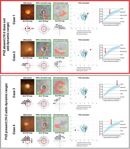
A prospective patient’s results may be compared to the present cohort to appreciate where they may lay in the spectrum. The use of the spreadsheet is demonstrated using four naïve cases that were not included in the development cohort in Figure 7. The top two cases (red box) demonstrate cases where an FVZ is unlikely to be present (where the defect on the 10-2 is more extensive than the 24-2; Figure 7, Cases 1 and 2). In Cases 1 and 2, the 24-2 has identified a similar pattern of defect to the 10-2 (an arcuate like defect paracentrally). The 10-2 test grid has proportionally more defects in the superior arcuate region, and thus, such locations are not likely to add further information on dynamic range. The bottom two cases (grey box) show situations where an FVZ is likely to be present (Figure 7, Cases 3 and 4; further details are in the Supplementary Material). Again, similar defects are identified using both test grids. However, the defect is notably deep when using the 24-2, whilst the 10-2 has proportionally fewer defects found in the same pattern. Therefore, the 10-2 has more residual test locations remaining, which could serve to track further disease progression.

Figure 7. Case examples of the application of the Functional Vulnerability Zone (FVZ) probability calculator and the simplified model (from Figure 6) to four naïve cases outside of the cohort used to construct the model. For the calculator, the position of the red dot (prospective patient) relative to the white (non-FVZ) and blue (FVZ) clusters indicate the likelihood of an FVZ being present. The simplified model shows the likelihood that an FVZ may be present, with the red arrows indicating the number of 24-2 central defects for each case. The top two cases (red box) indicate situations where an FVZ is not likely to be present (red dot is in the upper right quadrant on the calculator). The bottom two cases (grey box) indicate situations where an FVZ is likely to be present (red dot is in the left and lower regions). Key clinical findings are shown for each case, including optic nerve head (ONH) photographs, retinal nerve fibre layer (RNFL) deviation map,GanglionCellAnalysis (GCA) deviation map, 24-2 pattern deviation (PD) probability map, 24-2 numerical total deviation (TD) map and 10-2 PD map. Full case details are presented in the Supplementary Material.

The spreadsheet is not intended to be prescriptive, which is why a clear FVZ boundary is not explicitly defined. Instead, its purpose is to guide the clinician as to the likelihood or probability, based on the distribution of results, of the 10-2 test grid facilitating the future monitoring of residual visual field sensitivity. As described above, this shows the application of the simplified model presented in Figure 6, and also the limitations of relying solely on one metric from the 24-2 without knowledge about the 10-2 locations that may be affected.

Limitations

The study utilised cross-sectional data from the clinic to propose a model that compared the test grids. Longitudinal data would be beneficial for directly comparing the grids but would necessitate very long-term data to fully appreciate the spectrum of change towards the measurement floor. The authors specifically examined patients with defects on both test grids and did not include patients without central defects, as described in the inclusion and exclusion criteria. This was to represent a clinical scenario in which a clinician, presented with both options, aims to understand which would be preferable for the patient. This model requires long-term evaluation using a dataset with concurrent 24-2 and 10-2 to test its validity and would further benefit from a data set in which there was more indiscriminate 10-2 and 24-2 paired data obtained from a more naïve patient cohort. As mentioned in the Methods, repeatable test data, whilst desirable for confirming defects, was not the goal of the study, but could potentially be additive to future models. Similarly, this work represents a pilot study which needs further expansion with a larger and more diverse data set, and data from other clinical settings which would be necessary to assess external validity.

Development of this model was limited to using fixed grids available on the Humphrey Field Analyzer, and did not add custom test locations, such as with 1° spacing. For example, Numata and colleagues⁴⁸ performed a comprehensive static perimetry study using 0.5° spacing along a single meridian, suggesting that < 1.5° resolution is preferred for characterising very small scotomata in the central (10°) visual field. However, as further complexity and custom, non-standard grids are introduced, it would likely stray farther from clinical utility and pragmatism using current clinically available techniques. Similarly, the authors recognise the importance of relatively peripheral visual field loss in glaucoma, and that such defects require testing using a 24-2 or similar grid, rather than 10-2, for ongoing monitoring.

The goal of the present study was to create a model or framework upon which future empirical clinical data can be applied. There are several areas that require further exploration to further refine the developed model. These include the incorporation of test-retest variability, which may substantially affect defect detection, and an understanding of the sensitivity brackets or steps within the central visual field (as the brackets used in the present study were extrapolated from the work of Wall and colleagues⁴⁹ who used the 24-2; see Supplementary Material). A relevant practical concern related to progression analysis is the lack of commercially available methods such as Guided Progression Analysis for the 10-2.

Finally, the authors limited the assessment to two commonly used visual field test grids on the Humphrey Field Analyzer: the 24-2 and 10-2. The advantage of comparing these grids is their uniform arrangement and fixed distance between test locations, which allows for simpler comparisons. Simultaneously, it is known that 24-2 and 10-2 can return subtly different sensitivity results despite the mutuality of some test locations. A sanity test conducted supplementarily demonstrated moderate-to-strong correlations in the mutual test locations (Supplementary Figure 11). Although this represents a limitation of the commercial hardware, the authors propose that these differences would be reflective of routine clinical practice as these are clinically available test grids and algorithms. Other devices have other alternative test grid arrangements and would require further evaluation. A recent commercially available test grid on the same perimeter, the 24-2C, assesses test locations found on the 24-2 with an additional 10, asymmetrically distributed locations within the central 20 degrees. However, recent works have suggested no significant benefit of the 24-2C for identification of central visual field defects over the 24-2 or 10-2,^20,21,50 and the asymmetric distribution of test locations confounds contiguity analysis.

Conclusion

In this pilot study, the authors describe the visual field FVZ, and propose several quantitative markers that may suggest when a 10-2 may be clinically useful for examining a central visual field defect for the purposes of maximising dynamic range. The proposed markers include: 1) when there are 5 or more defective locations found in the central visual field in the 24-2; 2) when, in the context of central visual field defects, the mean deviation of the 10-2 is less severe (more positive) compared to the 24-2; and 3) when there are fewer than four 10-2 test locations affected for every one 24-2 test location with a defect.

Disclosure statement

No potential conflict of interest was reported by the author(s).

Supplementary data

Supplemental data for this article can be accessed online at https://doi.org/10.1080/08164622.2023.2288183.

Additional information

Funding

This work was supported in part by a National Health and Medical Research Council Ideas Grant [1186915] to MK and JP. Guide Dogs NSW/ACT provides funding for clinical services delivered at the Centre for Eye Health, where the patient data was collected. The funding body played no role in the conception or conduct of the study.

References

- Phu J, Agar A, Wang H et al. Management of open-angle glaucoma by primary eye-care practitioners: toward a personalised medicine approach. Clin Exp Optom 2021; 104: 367–384. doi:10.1111/cxo.13114.
- Prum BE Jr., Rosenberg LF, Gedde SJ et al. Primary open-angle glaucoma preferred practice pattern((R)) guidelines. Ophthalmology 2016; 123: 41–P111. doi:10.1016/j.ophtha.2015.10.053.
- Lee GA, Kong GYX, Liu CH. Visual fields in glaucoma: where are we now? Clin Exp Ophthalmol 2023; 51: 162–169. doi:10.1111/ceo.14210.
- Jampel HD, Singh K, Lin SC et al. Assessment of visual function in glaucoma: a report by the American academy of ophthalmology. Ophthalmology 2011; 118: 986–1002. doi:10.1016/j.ophtha.2011.03.019.
- Phu J, Khuu SK, Yapp M et al. The value of visual field testing in the era of advanced imaging: clinical and psychophysical perspectives. Clin Exp Optom 2017; 100: 313–332. doi:10.1111/cxo.12551.
- Schiefer U, Papageorgiou E, Sample PA et al. Spatial pattern of glaucomatous visual field loss obtained with regionally condensed stimulus arrangements. Invest Ophthalmol Visual Sci 2010; 51: 5685–5689. doi:10.1167/iovs.09-5067.
- Khoury JM, Donahue SP, Lavin PJ et al. Comparison of 24-2 and 30-2 perimetry in glaucomatous and nonglaucomatous optic neuropathies. J Neuroophthalmol 1999; 19: 100–108. doi:10.1097/00041327-199906000-00004.
- Heijl A, Patella VM, Chong LX et al. A New SITA perimetric threshold testing algorithm: construction and a multicenter clinical study. Am J Ophthalmol 2019; 198: 154–165. doi:10.1016/j.ajo.2018.10.010.
- Phu J, Khuu SK, Agar A et al. Clinical evaluation of Swedish interactive thresholding algorithm-faster compared with Swedish interactive thresholding algorithm-standard in normal subjects, glaucoma suspects, and patients with glaucoma. Am J Ophthalmol 2019; 208: 251–264. doi:10.1016/j.ajo.2019.08.013.
- Blumberg DM, De Moraes CG, Prager AJ et al. Association between undetected 10-2 visual field damage and vision-related quality of life in patients with glaucoma. JAMA Ophthalmol 2017; 135: 742–747. doi:10.1001/jamaophthalmol.2017.1396.
- Yamazaki Y, Sugisaki K, Araie M et al. Relationship between vision-related quality of life and central 10 degrees of the binocular integrated visual field in advanced glaucoma. Sci Rep 2019; 9: 14990. doi:10.1038/s41598-019-50677-0.
- Sun Y, Lin C, Waisbourd M et al. The impact of visual field clusters on performance-based measures and vision-related quality of life in patients with glaucoma. Am J Ophthalmol 2016; 163: 45–52. doi:10.1016/j.ajo.2015.12.006.
- White A, Goldberg I. Australian and New Zealand glaucoma interest group and the Royal Australian and New Zealand college of ophthalmologists guidelines for the collaborative care of glaucoma patients and suspects by ophthalmologists and optometrists in Australia. Clin Exp Ophthalmol 2014; 42: 107–117. doi:10.1111/ceo.12270.
- Traynis I, De Moraes CG, Raza AS et al. Prevalence and nature of early glaucomatous defects in the central 10 degrees of the visual field. JAMA Ophthalmol 2014; 132: 291–297. doi:10.1001/jamaophthalmol.2013.7656.
- De Moraes CG, Hood DC, Thenappan A et al. 24-2 visual fields miss central defects shown on 10-2 tests in glaucoma suspects, ocular hypertensives, and early glaucoma. Ophthalmology 2017; 124: 1449–1456. doi:10.1016/j.ophtha.2017.04.021.
- West ME, Sharpe GP, Hutchison DM et al. Value of 10-2 visual field testing in glaucoma patients with early 24-2 visual field loss. Ophthalmology 2021; 128: 545–553. doi:10.1016/j.ophtha.2020.08.033.
- Sullivan-Mee M, Karin Tran MT, Pensyl D et al. Prevalence, features, and severity of glaucomatous visual field loss measured with the 10-2 achromatic threshold visual field test. Am J Ophthalmol 2016; 168: 40–51. doi:10.1016/j.ajo.2016.05.003.
- Wu Z, Medeiros FA, Weinreb RN et al. Performance of the 10-2 and 24-2 visual field tests for detecting central visual field abnormalities in glaucoma. Am J Ophthalmol 2018; 196: 10–17. doi:10.1016/j.ajo.2018.08.010.
- Orbach A, Ang GS, Camp AS et al. Qualitative evaluation of the 10-2 and 24-2 visual field tests for detecting central visual field abnormalities in glaucoma. Am J Ophthalmol 2021; 229: 26–33. doi:10.1016/j.ajo.2021.02.015.
- Phu J, Kalloniatis M. Comparison of 10-2 and 24-2C test grids for identifying central visual field defects in glaucoma and suspect patients. Ophthalmology 2021; 128: 1405–1416. doi:10.1016/j.ophtha.2021.03.014.
- Phu J, Kalloniatis M. Ability of 24-2C and 24-2 grids to identify central visual field defects and structure-function concordance in glaucoma and suspects. Am J Ophthalmol 2020; 219: 317–331. doi:10.1016/j.ajo.2020.06.024.
- Wu Z, Medeiros FA, Weinreb RN et al. Comparing 10-2 and 24-2 visual fields for detecting progressive central visual loss in glaucoma eyes with early central abnormalities. Ophthalmol Glaucoma 2019; 2: 95–102. doi:10.1016/j.ogla.2019.01.003.
- Susanna FN, Melchior B, Paula JS et al. Variability and power to detect progression of different visual field patterns. Ophthalmol Glaucoma 2021; 4: 617–623. doi:10.1016/j.ogla.2021.04.004.
- Mikelberg FS, Drance SM. The mode of progression of visual field defects in glaucoma. Am J Ophthalmol 1984; 98: 443–445. doi:10.1016/0002-9394(84)90128-4.
- Werner EB, Drance SM, Schulzer M. Trabeculectomy and the progression of glaucomatous visual field loss. Arch Ophthalmol 1977; 95: 1374–1377. doi:10.1001/archopht.1977.04450080084008.
- Morin JD. Changes in the visual fields in glaucoma: static and kinetic perimetry in 2,000 patients. Trans Am Ophthalmol Soc 1979; 77: 622–642.
- Nevalainen J, Paetzold J, Papageorgiou E et al. Specification of progression in glaucomatous visual field loss, applying locally condensed stimulus arrangements. Graefes Arch Clin Exp Ophthalmol 2009; 247: 1659–1669. doi:10.1007/s00417-009-1134-2.
- Ly A, Wong E, Huang J et al. Glaucoma community care: does ongoing shared care work? Int J Integr Care 2020;20:5. doi:10.5334/ijic.5470.
- Huang J, Yapp M, Hennessy MP et al. Impact of referral refinement on management of glaucoma suspects in Australia. Clin Exp Optom 2020; 103: 675–683. doi:10.1111/cxo.13030.
- Wang H, Kalloniatis M. Clinical outcomes of the centre for eye health: an intra-professional optometry-led collaborative eye care clinic in Australia. Clin Exp Optom 2021; 104: 795–804. doi:10.1080/08164622.2021.1878821.
- Phu J, Kalloniatis M. A strategy for Seeding Point Error Assessment for Retesting (SPEAR) in perimetry applied to normal subjects, glaucoma suspects, and patients with glaucoma. Am J Ophthalmol 2021; 221: 115–130. doi:10.1016/j.ajo.2020.07.047.
- Phu J, Kalloniatis M. Viability of performing multiple 24-2 visual field examinations at the same clinical visit: the Frontloading Fields Study (FFS). Am J Ophthalmol 2021; 230: 48–59. doi:10.1016/j.ajo.2021.04.019.
- Garway-Heath DF, Quartilho A, Prah P et al. Evaluation of visual field and imaging outcomes for glaucoma clinical trials (an American ophthalomological society thesis). Trans Am Ophthalmol Soc 2017; 115: T4.
- Hood DC, Raza AS, de Moraes CG et al. Glaucomatous damage of the macula. Prog Retin Eye Res 2013; 32: 1–21. doi:10.1016/j.preteyeres.2012.08.003.
- Choi AYJ, Nivison-Smith L, Phu J et al. Contrast sensitivity isocontours of the central visual field. Sci Rep 2019; 9: 11603. doi:10.1038/s41598-019-48026-2.
- Artes PH, Iwase A, Ohno Y et al. Properties of perimetric threshold estimates from full threshold, SITA standard, and SITA fast strategies. Invest Ophthalmol Visual Sci 2002; 43: 2654–2659.
- Gardiner SK, Swanson WH, Goren D et al. Assessment of the reliability of standard automated perimetry in regions of glaucomatous damage. Ophthalmology 2014; 121: 1359–1369. doi:10.1016/j.ophtha.2014.01.020.
- Phu J, Khuu SK, Agar A et al. Visualizing the consistency of clinical characteristics that distinguish healthy persons, glaucoma suspect patients, and manifest glaucoma patients. Ophthalmol Glaucoma 2020; 3: 274–287. doi:10.1016/j.ogla.2020.04.009.
- Rafla D, Khuu SK, Kashyap S et al. Visualising structural and functional characteristics distinguishing between newly diagnosed high-tension and low-tension glaucoma patients. Ophthalmic Physiol Opt 2023; 43: 771–787. doi:10.1111/opo.13129.
- Yang SH, Liu R. Four decades of ischemic penumbra and its implication for ischemic stroke. Transl Stroke Res 2021; 12: 937–945. doi:10.1007/s12975-021-00916-2.
- Boden C, Blumenthal EZ, Pascual J et al. Patterns of glaucomatous visual field progression identified by three progression criteria. Am J Ophthalmol 2004;138:1029–1036. doi:10.1016/j.ajo.2004.07.003.
- Aulhorn E, Harms H. Early visual field defects in glaucoma. Basel: Karger; 1967.
- Westcott MC, McNaught AI, Crabb DP et al. High spatial resolution automated perimetry in glaucoma. Br J Ophthalmol 1997; 81: 452–459. doi:10.1136/bjo.81.6.452.
- Aoyama Y, Murata H, Tahara M et al. A method to measure visual field sensitivity at the edges of glaucomatous scotomata. Invest Ophthalmol Visual Sci 2014; 55: 2584–2591. doi:10.1167/iovs.13-13616.
- Tomairek RH, Aboud SA, Hassan M et al. Studying the role of 10-2 visual field test in different stages of glaucoma. Eur J Ophthalmol 2020; 30: 706–713. doi:10.1177/1120672119836904.
- Park SC, Kung Y, Su D et al. Parafoveal scotoma progression in glaucoma: humphrey 10-2 versus 24-2 visual field analysis. Ophthalmology 2013; 120: 1546–1550. doi:10.1016/j.ophtha.2013.01.045.
- Rao HL, Begum VU, Khadka D et al. Comparing glaucoma progression on 24-2 and 10-2 visual field examinations. PLoS ONE 2015; 10: e0127233. doi:10.1371/journal.pone.0127233.
- Numata T, Matsumoto C, Okuyama S et al. Detectability of visual field defects in glaucoma with high-resolution perimetry. J Glaucoma 2016; 25: 847–853. doi:10.1097/IJG.0000000000000460.
- Wall M, Zamba GKD, Artes PH. The effective dynamic ranges for glaucomatous visual field progression with standard automated perimetry and stimulus sizes III and V. Invest Ophthalmol Visual Sci 2018; 59: 439–445. doi:10.1167/iovs.17-22390.
- Chakravarti T, Moghadam M, Proudfoot JA et al. Agreement between 10-2 and 24-2C visual field test protocols for detecting glaucomatous central visual field defects. J Glaucoma 2021; 30: e285–e91. doi:10.1097/IJG.0000000000001844.