ARTIFICIAL INTELLIGENCE AND GRAPH THEORY TOOLS FOR DESCRIBING SWITCHED LINEAR CONTROL SYSTEMS

Abstract

This paper develops a representation of multi-model based controllers using artificial intelligence techniques. These techniques will be graph theory, neural networks, genetic algorithms, and fuzzy logic. Thus, graph theory is used to describe in a formal and concise way the switching mechanism between the various plant parameterizations of the switched system. Moreover, the interpretation of multi-model controllers in an artificial intelligence frame will allow the application of each specific technique to the design of improved multi-model based controllers. The obtained artificial intelligence-based multi-model controllers are compared with classic single model-based ones. It is shown through simulation examples that a transient response improvement can be achieved by using multi-estimation based techniques. Furthermore, a method for synthesizing multi-model-based neural network controllers from already designed single model-based ones is presented, extending the applicability of this kind of technique to a more general type of controller. Also, some applications of genetic algorithms and fuzzy logic to multi-model controller design are proposed. In particular, the mutation operation from genetic algorithms inspires a robustness test, which consists of a random modification of the estimates which is used to select the one leading to the better identification performance towards parameterizing online the adaptive controller. Such a test is useful for plants operating in a noisy environment. The proposed robustness test improves the selection of the plant model used to parameterize the adaptive controller in comparison to classic multi-model schemes where the controller parameterization choice is basically taken based on the identification accuracy of each model. Moreover, the fuzzy logic approach suggests new ideas to the design of multi-estimation structures, which can be applied to a broad variety of adaptive controllers such as robotic manipulator controller design.

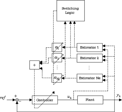
Adaptive control is a well-known control method which allows to stabilize dynamical system with partially or totally unknown parameters as well as the achievement of acceptable tracking performances (VanDoren 2003; Aström and Wittenmark 1995). The designed adaptive controllers have been successfully used when the plant has unknown but constant parameters as well as when the plant is time-varying provided that the variation of its parameters is slower than the adaptation rate of the adaptive scheme. Nevertheless, sudden changes in the plant operating point, which entail a sudden change in the plant parameter values, are not surprising in many industrial applications such as in certain chemical engineering processes or electric motors (Cezayirli and Ciliz 2004). If a single identification model is used, then the system will have to adapt itself to the new situation before an adequate control action can be taken. Hence, single model-based adaptive controllers may lead to a poor transient response in terms of the plant output deviation from a reference one in these situations. Furthermore, an inadequate initialization of the estimated plant parameters in the estimation algorithm may result in unacceptable large transient deviations. Thus, multi-estimation-based controllers appeared as a way to improve the transient response of adaptive systems (Narendra and Balakrishnan 1994; Gregorcic et al. 2001; Chang and Davison 1999; Narendra and Balakrishnan 1997; Mosca and Agnoloni 2001; Hocherman-Frommer et al. 1998; Ibeas et al. 2003) by considering a set of parameter estimation algorithms running in parallel, each one being initialized by a different set of estimated plant parameter values. This mechanism allows to quickly correct any potential erroneous choice of the initial values of the plant parameters selected to start to run the estimation algorithm due to a convenient parameterization of the adaptive controller by adequate switching between estimators. Moreover, the existence of a set of estimation algorithms running in parallel allows to improve the control action when the plant changes its operation point abruptly by a convenient switching to an estimator closer to the new plant parameterization (Ibeas et al. 2003; Cezayirli and Ciliz 2004). A general multi-model-based control scheme is composed of a set of different plant models running in parallel. These models, which may be fixed (Narendra and Balakrishnan 1994; Gregorcic et al. 2001; Chang and Davison 1999) or adaptive (Narendra and Balakrishnan 1997; Mosca and Agnoloni, 2001; Hocherman-Frommer et al. 1998; Ibeas et al. 2003) are different from each other in what is concerned with their structure and/or their parameter values. Then, a higher level switching structure between the various plant models chooses, according to a closed-loop performance index built for each one, the one used to calculate the control law at that time instant. In Mosca and Agnoloni (2001) and Hocherman-Frommer et al. (1998), several performance indexes for that purpose are discussed. Despite the specific form of the performance index is different from one work to another, it is common to define it based on the error between the real plant output and each model's one, which is a natural choice since that index reflects how far a specific model is from the real plant behavior. Thus, the switching law acts as a supervisor of the system behavior deciding in real time the estimator that will parameterize the adaptive controller. Hence, this kind of control architecture allows to develop control system schemes capable of achieving a good performance in terms of speed, accuracy, and stability for increasingly complex systems (Ibeas et al. 2003; Sun and Ge 2003; Cezayirli and Ciliz 2004; Chen and Narendra 2001).

The structure and operation of the switching law have been previously studied from an artificial intelligence point of view in an expert systems context (de la Sen et al. 2004; de la Sen and Almansa 2002). In addition, this paper proposes a formal interpretation of the multi-model (multi-estimation in the more general case concerned with adaptive models) switching structure in a more general artificial intelligence frame. First, the switching mechanism between plant models is described using a graph theory-based formalism. A graph containing information about the number of estimators running in parallel as well as the possibility of switching between them is introduced. The concept of extended adjacency matrix is proposed and used to describe the way in which the switching law between estimators is implemented and defined in a practical multiestimation scheme. An adaptive, being a more general case than that concerned with fixed models, will be used to represent the formalism. Thus, the switching rule is completely described by the proposed graph while the realization of the switching rule in a concrete simulation example leads to a walk in this graph. Once a general formalism representing the switching scheme is stated, the multi-estimation scheme is represented by using artificial intelligence typical structures such as: artificial neural networks (ANN), genetic algorithms (GA), and fuzzy logic (Da Ruan 1997; Fausett 1998; Etxebarria 1994; Beyers 1998; Tilli 1992; Ibeas and de la Sen 2004). This interpretation will allow the use of specific characteristics of each technique to the design of improved multi-model control schemes. Thus, a method for synthesizing multi-model-based neural network controllers from previously designed single model ones is proposed. Also, a complete multi-estimation-based control scheme built using ANN technology entirely is described. Since there are a number of estimation algorithms running in parallel, only one parameterizing the adaptive controller at each time instant, we can use the selected estimation algorithm to guide the rest of them to a possibly improved estimated parameter vector. The way for implementing this issue is to modify the estimated parameter vector updating equation to include a term which monitors the updating process in the direction of the selected current best estimated vector. Moreover, some applications of genetic algorithms and fuzzy logic to multi-model control design are presented. The genetic algorithm approach will inspire the incorporation of a robustness measure of each model in the performance index used for evaluating the closed-loop behavior of the set of estimation algorithms running in parallel. The robustness test consists of a random perturbation of the estimated plant parameter vector values in order to select which one of them leads to a better identification performance under random modification of its values. Thus, the resulting scheme will be able to improve its transient behavior in comparison to the classic multi-model schemes, where this robustness measure is not included, when the plant is operating in a noisy environment as computer simulations have shown. Furthermore, a fuzzy logic approach is presented to interpret the architecture of multi-estimation-based controllers. This problem focusing way can be applied to the design of multi-model controllers, as recent works (Ibeas and de la Sen 2004; de la Sen and Almansa 2002; Ibeas et al. 2004) use in the control of uncertain robotic manipulators. Each representation will be compared with the traditional single model-based adaptive controller design in order to illustrate the usefulness of the proposed schemes.

PRELIMINARIES ON SWITCHED LINEAR SYSTEMS

In this section, a brief description of the switched linear control scheme used for subsequent discussion is presented. The discussion has been restricted to linear systems to avoid the existence of finite escape times. Thus, a switched linear system is described (unifying the notation for the continuous and discrete time systems) by:

where x(t) ∈ ℝ ⁿ are the states, u _σ(t) ∈ ℝ ^p are the control inputs with σ ∈ M = {1, 2,…, N _e }(x(t _k ) = x _k , u(t _k ) = u _k for the discrete cases respectively), δ denotes the time derivative d/dt for the continuous case and the difference operator (q − 1)/T (being q the one-step time-forward operator and T the sampling period) for the discrete time case, and A _σ, B _σ are matrices of compatible dimensions. This formulation allows to consider in a unified way both the continuous and discrete cases with the use of a combined notation. Also, σ : ℝ ⁿ  × ℝ × M → M is the switching signal, which selects the model from the set of N _e models parameterizing (1) at each time instant. In general, the switching signal σ may depend on the state, time, and on its previous value. It is said that the switching signal is well-defined or the switched system is well posed (Sun and Ge 2003; Sun 2004) if for any bounded initial state x(t ₀) = x ₀, the switched system has a solution for all subsequent time t > t ₀ and it implies a finite number of switches in a finite time interval. Note that this definition implies the existence of a minimum residence time of a plant model parameterizing the system before any switching can occur, or in other words, the switching signal is not allowed to switch infinitely fast. This notation also implies that the switching may affect the control input u _σ, which is the typical case in many switching systems as in the case of adaptive multi-estimation-based schemes, in which the switching rule selects the estimation algorithm used to parameterize an adaptive controller. Moreover, it is typical to define a supervisory index at each time instant for each plant estimator (model) running in parallel, in order to evaluate the goodness of each model to parameterize the overall system. This index evaluates the goodness of jth model (as a potential model to parameterize the system) when the ith model has been parameterizing the system during the previous residence time interval. Once the minimum residence time constraint has been fulfilled, the selected model to parameterize the adaptive controller is determined by evaluating the estimator, which leads to the minimum of such functions.

Architecture of an Adaptive Multi-Estimation Scheme for Discrete Linear Systems

In this section, a case study of a multi-estimation-based control scheme for linear discrete systems is presented. Even if multi-model control schemes can be applied either to continuous or discrete systems (as Equation (1) highlights), the following discrete example will be used through the work to illustrate the presented artificial intelligence formalism in a concrete control scheme. Thus, our objective is to design a model reference following pole placement-based multi-estimation-based control for the discrete (the continuous case can be treated in the same way) time invariant linear SISO plant:

where U(z), Y(z) are the z-transforms of the input and output sequences u _k , y _k , respectively, being the z indeterminate formally analogous to the one-step time-forward operator and

where n ≥ m ≥ 0. Furthermore, note that Equations (2–3) define a linear difference equation which is usually written in adaptive control as the inner product of two vectors (Etxebarria 1994; Aström and Wittenmark 1995):

where

is the so called regressor and

symbolizes the true plant parameter vector (Ibeas et al. 2003). This plant is an example of how the presented methodology can be applied to a concrete problem. Furthermore, in Ibeas and de la Sen (2004); de la Sen et al. (2003); Sun and Ge (2003); Sun (2004); and Chen and Narendra (2001), you can find the development of multi-model controllers to more general types of uncertain dynamical systems. However, in order to illustrate the application of the proposed representations to a concrete problem in an easy way, the linear difference plant has been chosen. If the true plant parameter vector is unknown, then parameter estimation has to be used. Thus, an estimated parameter vector k is considered at each sample k provided by any parameter estimation algorithm. The estimated parameter vector generates an estimated plant output through an equation analogue to (4):

Then, this estimated parameter vector k is used for control law calculations at each sample by using the certainty equivalence principle (Aström and Wittenmark 1995). If this estimated vector is initialized far from the real plant parameter vector, then the transient response will have large deviations from the desired output, resulting in a bad transient tracking performance. Furthermore, if during the system operation, the plant's operating point changes abruptly at certain time instants, then the system will exhibit an unsuitable transient response. These facts motivate the consideration of a set of estimation algorithms running in parallel, each one with its own estimated plant parameter vector:

where N _e is the number of total estimators. Each estimated vector is updated at each sample, according to a parameter estimation algorithm driven by the input and output measurements of the plant. The multi-estimation scheme block diagram is displayed in Figure 1.

FIGURE 1 Basic multi-estimation scheme architecture.

Thus, there exists N _e estimation algorithms running in parallel (i.e., at each sampling time t _k  = kT, T being the sampling period, every algorithm gives the estimate parameter vector and the estimated plant output , based on past plant input and output measurements). Each algorithm is different from each other in what is concerned with the estimated parameter vector initialization and/or the kind of the estimation algorithm and integrates the so-called multi-estimation scheme. Denote by c _k the identification algorithm which parameterizes the adaptive controller at time t _k . A switching rule based on the identification errors , of the N _e estimation algorithms chooses at each sampling time t _k the individual estimation scheme (identifier) c _k , which parameterizes the active controller at time t _k . Thus, any potential erroneous choice of the initial estimated plant parameter vector is quickly corrected by the switching structure via looking for the “best” estimation model. Moreover, when the system changes its operation point, and this fact is detected through a monitorizing index according to a prescribed threshold, then all the estimation algorithms are reset to their original locations and uniformly distributed over the known, convex, and compact parameter space. Hence, when a change in the plant parameters happens, then the system is able to select the most convenient parameterization of the adaptive controller to achieve an adequate closed-loop transient performance (Ibeas et al. 2003). The proposed identification performance supervisory index for each estimation algorithm used for selecting the current one to parameterize the adaptive controller (once the minimum residence time constraint is fulfilled) is:

where H is a positive integer number large enough to give sense to the performance evaluation and c : ℝ → Mwithc _k  ∈ M = {1, 2,…, N _e }. Thus, index (6) can be interpreted as the switching evaluation index of the ith estimator when the previous estimator parameterizing the system has been the c _k−1 − th. Moreover, the first addend of index (6) can be interpreted as a measure of the long-term accuracy of each identification algorithm, where the forgetting factor λ_ℓ ∈ (0, 1) (which, in general, can be sample-dependent) establishes the effective memory of the index in rapidly changing environments. The second part of the index (6) can be interpreted as the possible jump in the control law associated to switching between controller parameterizations. The supervisory index is built through a convex linear combination of the previous terms as it is highlighted by Equation (6). Moreover, the real plant parameter vector is not used in any calculation since the identification error may be equivalently written as being a measurable signal since the real plant output is measured. The switching law must respect a minimum dwell or residence time between consecutive switchings between estimators in order to guarantee closed-loop stability (Narendra and Balakrishnan 1997; Ibeas et al. 2003). Furthermore, once the supervisory index (6) has been stated, the switching rule for the adaptive controller reparameterization is obtained from the minimization of the identification supervision index (6) as follows. Switching is not allowed and the current controller is maintained in operation while the elapsed time from the last switching is smaller than the minimum residence time. On the other hand, if the elapsed time from the last switching is larger than or equal to the residence time, then switching is allowed. In this case, the controller chosen from the multi-estimation scheme is such that it has the minimum performance index (6) from all pairs of estimator-controller parameterization available. If two estimators have the same performance index, then the selected controller is the one with the minimum index in the ordered set M = {1, 2,…, N _e }. The switching process is described by the following algorithm:

	Algorithm 1. (Switching Between Estimators)
	{k = 0;N r  > 0, c 0, selected by the designer, ST = Ø(The Initial Switching Samples Sequence Is Empty)}
	k lastSwitch  = 0
	for k > 0 do
	if (k − k lastSwitch ) ≥ N r then
	c k  ←  k
	if c k  ≠ c k−1 then
	ST ← ST ∪ {k}, klastSwitch ← k end_if
	else
	ck= ck − 1
	end_if
	end_for
	{the current estimation algorithm parameterizing the adaptive controller c k is determined},

where N _r (positive integer) is the residence number of samples, which is related to the minimum residence time through T _r  = N _r T, and ST is the set containing the sequence of switching samples. Then, the selected estimated parameter vector is used for parameterization of the adaptive controller and generation of the plant input. Thus, the parallel multi-estimation scheme is used to improve the transient response of single model-based adaptive controllers through appropriate switching to a more convenient parameterization of the controller. Furthermore, the proposed control methodology has been applied to discrete plants with unmodeled dynamics (de la Sen et al. 2003), and even to continuous nonlinear dynamical systems such as robot manipulators (Ibeas and de la Sen 2004; Chen and Narendra 2001). Since the main objective of this paper is to develop an artificial intelligence representation of multi-model structures rather than describing the control scheme, the reader is referred to (Ibeas et al. (2003), where a complete discussion of the stability issues and the pole placement adaptive control design is available. Moreover, it is proved in this work that the closed-loop system can be written in the general form given by (1), considering the control law and an extended state vector composed of the output and the control input. The switching rule design has been focused from an expert systems formalism in previous works (de la Aen et al. 2004; de la Sen and Almansa 2002). Now the switching mechanism as well as multi-estimation structures are represented in a more general artificial intelligence frame in the following sections.

GRAPH THEORY-BASED REPRESENTATION OF THE SWITCHING PROCESS

In the following, a graph theory-based representation of the switching process is stated. Previously to such a representation, a brief background on graph theory is introduced.

Brief Background and Notation on Graph Theory

A brief background and notation on graph theory is now given to make the subsequent representation clear (Chartrand and Lesniak 1979; Diestel 2000). A graph (digraph or directed graph) is a pair G = (V, E)(G = (V, A) for digraphs) consisting in a finite nonempty set V of objects called vertices together with a (possible empty) set of unordered pairs (ordered pairs for the case of digraphs) of distinct vertices of V called edges (arcs or directed edges). The edge e = {u, v} ∈ E is said to join the vertices u ∈ V and v ∈ V. If e = {u, v} is an edge of the graph G, then u and v are adjacent vertices. Moreover, a loop graph is defined as a nonempty set V of vertices together with a (possible empty) set E of edges consisting of one or two element subsets of V, each one-element subset is referred to as a loop. A loop graph that admits multiple edges (including multiple loops) is called a pseudograph. Furthermore, a pseudograph is extended to a pseudo-digraph by considering arcs instead of edges to join vertices. The number of vertices is called the cardinal of V (or the degree or power of the graph G). A walk in G is defined by:

The complete graph of degree n, denoted by K _n , is defined as the graph in which every two of its vertices are adjacent (the complete symmetric digraph or order n, denoted by K _n *, has both arcs (u, v) and (u, v) for every two distinct vertices u, v ∈ V). The complete pseudograph K _pn and the complete symmetric pseudo-digraph K _pn * are obtained by adding a loop (being an edge or an arc respectively) to all vertices in V. The adjacency matrix of a digraph G = (V, A) with n vertices is the n × n matrix [a _ij ] defined by a _ij  = 1 if (v _i , v _j ) ∈ E(A) and a _ij  = 0 otherwise. A weighted graph (weighted digraph) is a graph (digraph) in which a positive real number, called the weight of e (a) and denoted by w(e) (w(a)) is assigned to each edge (arc) e ∈ E(a ∈ A). The adjacency matrix concept can be extended to weighted graphs by considering the weighted adjacency matrix [a _ij ] defined by a _ij  = w(e(a)), if e(a) = (v _i , v _j ) ∈ E(A) and a _ij  = 0 otherwise.

Graph Theory-Based Representation of the Switching Law

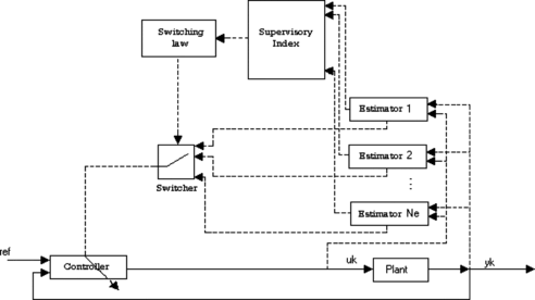
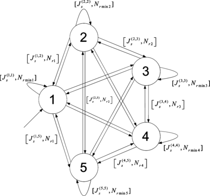
A graph theory-based description of the switching subsystem described by Equations (1) is now given which is then used to describe the general adaptive multiestimation scheme described previously. Basically, the vertices of the graph represent estimation algorithms (or equivalently parameterizations of the dynamical system (1)) while the arcs represent switches between different estimators. Auto loops are used to highlight the fact that a minimum residence time at each active estimation algorithm (or system parameterization) has to be respected in order to make the switching law well posed. Now, the switching law of the multi-estimation scheme displayed in Figure 1, composed of N _e estimation algorithms running in parallel, can be represented by a complete symmetric pseudo-digraph, called a switching graph, constructed using the following rules:

	Rule 1. Consider the complete symmetric pseudo-digraph of order N e , .
	Rule 2. Select one vertex as the starting vertex marking it with an arrow. This rule may be interpreted as the selection of the initial estimation algorithm chosen to start to run the switched linear system.
	Rule 3. There is a vector weight associated with each arc between vertices whose first component is the (non-negative) supervisory index associated with the switching between both estimators, while its second component is the (positive) time associated with the residence time interval within which the system has been parameterized by the previous estimation scheme.
	Rule 4. There exists a vector weight associated with each auto loop composed of two components: The first one is the supervisory index of the current parameterization of the system if it does not switch to another parameterization once the residence time constraint has been fulfilled. The second one is the minimum residence time the switching mechanism is bound to maintain the current system parameterization active in order to guarantee the switching rule is well posed.

Remarks

1.	The proposed switching graph represents the operation mechanism of the switching process and, hence, it is a complete description of the switching rule. Thus, the graph represents a switching rule where the system is able to switch from one system parameterization to any other once the residence time constraint is fulfilled.
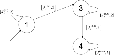
2.	A walk in this switching graph can be interpreted as a concrete realization of the switching rule applied to a particular case study.
3.	Note that the first superscript in the supervisory index (6) indicates the estimator which has been parameterizing the adaptive controller during the last residence time interval, while the second one labels the next estimator which potentially can parameterize the adaptive controller at the following time instant.

In order to represent the graph in a more formal way by using concepts and descriptions from the graph theory, the following definition of extended adjacency matrix is introduced:

Definition 1

The extended adjacency matrix of a pseudo-digraph G = (V, A) with card(V) = n is the square n × n matrix [a _ij ] whose entries are defined by the vector if (v _i ) ∈ A, if (v _i , v _j ) ∈ A and a _ij  = [0, 0] = 0_1×2. Otherwise, where N _rmini is the minimum residence time (minimum residence number of samples), a selected estimation algorithm must remain parameterizing the adaptive controller to guarantee the switching law is well posed, while N _ri is the real residence time (real residence number of samples) the selected estimation algorithm has been parameterizing the adaptive controller before switching to another estimation algorithm. Hence, the switching rule can be formally determined by defining the switching graph together with the extended adjacency matrix. For example, the extended adjacency matrix for a switching graph composed of five identifiers running in parallel is:

Remarks

1.

The extended adjacency matrix is not symmetric despite the digraph is topologically symmetric and complete. The main reason for this stands on that the supervisory index is different from since the system is being parameterized by the 2-th estimator within the residence time in the former, while the system is being parameterized by the third one in the latter. These supervisory indexes are dynamically determined through online measurements over the plant.

2.

Note that since the vector weights of the graph (in particular, the supervisory index ) are time varying; the extended adjacency matrix will also be time varying.

Example of the Graph Representation of the Switching Law

An example of the switching graph representation for the discrete SISO linear control scheme defined previously is developed. Consider the following system described by the (unknown for control purposes) plant:

which can be represented by the parameter vector θ ^T  = [1.4 − 0.95 0.510.1 − 0.3]. We will consider five estimation algorithms of least-squares type (Aström and Wittenmark 1995) running in parallel, whose equations are:

where ϕ _k is the defined regressor, 0⁽ⁱ⁾ arbitrary and bounded, and (bounded) for i = 1, 2,…, N _e and initialized by:

while the covariance matrix is initialized by . The first estimator is the one which starts parameterizing the adaptive controller. This example can be represented by the graph displayed in Figure 2. K _p5*, with the extended adjacency matrix defined, is the performance index (by choosing β₁ = 1, β₂ = 0 in (6)), where the forgetting factor is λ = 0.95 and N _rmini  = 2 samples ∀ i = 1, 2,…, 5. The reference signal is a square wave with a period of 20 samples and an amplitude of ±1.

FIGURE 2 Switching graph for a multi-model scheme composed of five models in parallel.

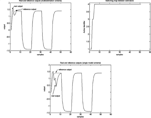
Figure 3 shows simulations of the multi-estimation control scheme.

FIGURE 3 Simulation example of a discrete multi-estimation-based scheme.

Moreover, the realization of the switching law over this concrete plant and multi-estimation scheme until time t = 50T has led the system to describe the path displayed in Figure 4.

FIGURE 4 Walk describing the realization of the switching graph in a concrete example.

ARTIFICIAL NEURAL NETWORKS

In this section, an artificial neural network (ANN) (Fausett 1998; Wang and Qing 2004; Etxebarria and de la Sen 1996; Melin and Castillo 2003) representation for the multi-estimation-based control scheme described previously is presented. First, we will introduce a possible representation of the parallel estimation scheme into a unique estimation neural network. Then, the architecture of the complete multi-estimation scheme will be formally described by using a set of different interconnected neural networks. Furthermore, the selected estimation algorithm chosen to parameterize the adaptive controller in real time is used for monitoring the evolution of the estimated parameter vectors of the remaining estimation algorithms running in parallel to the directions of this one which achieves a better closed-loop response.

ANN for Representing Single Estimation-Based Schemes

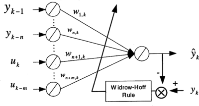
The following two-layered ANN is presented as a model for a discrete time single model-based adaptive control in Etxebarria (1994). The difference equation (2–3) is implemented by the ANN displayed in Figure 5, where the activation functions are linear for all neurons.

FIGURE 5 Single neural network estimator.

The ANN output (whose role is played by the estimated plant output) can be written as:

where w _k (with at least one component being non-zero) is the network weights vector and ϕ is the defined regressor. Comparing Equation (7) with Equation (5), it can be observed that the network weight vector w _k plays the same role as the estimated plant parameter vector k. Network weights (or equivalently plant parameters) are updated by using the well-known Widrow-Hoff rule for multiple-input, single-output ANN (Fausett 1998; Etxebarria 1994).

where ŷ _k denotes the ANN estimated plant output, while y _k denotes the real measured plant output (Etxebarria 1994). Thus, the network weights are updated by comparing the network output with the real plant output (which it is the target value). Then, the weights vector (whose role is represented by the estimated plant parameters vector) is used for controller design purposes. This neural network is extended to represent multi-estimation structures in the following section.

ANN for Representing Multi-Estimation Schemes

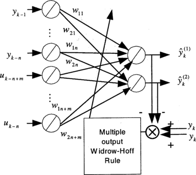
Now, the multi-estimation scheme introduced previously can be represented using an ANN by increasing the number of neurons in the output layer of the given ANN to a number of neurons equal to the number of different estimators used in the multi-estimation scheme. Since the output layer has one single neuron in the previous network, a multiestimation scheme with N _e estimators running in parallel will have N _e neurons in its output layer, as Figure 6 displays for the case of N _e  = 2.

FIGURE 6 Multi-estimation neural network.

Hence, the number of connections between neurons and the number of weights are increased. Thus, the proposed ANN is a unique structure containing itself the N _e estimated parameter vectors (which are represented by the corresponding weights vectors). Furthermore, the ANN plant estimated outputs are obtained as:

From the weight values w _{ij, k} , two estimated plant parameter vectors may be defined by . The target vector (with which the ANN is trained) is defined in this case by repeating the original target value as many times as the number of estimators used. Since the original target value was the real measured plant output, y _k , in the general case with N _e estimators, the new target vector will be:

Then the switching logic compares the performance indexes (6) associated to each output of the ANN and chooses the set of weights (estimated parameter vector) associated with the best estimated output, according to the controller selection algorithm described previously in order to calculate the control signal. The training rule is the generalization of the Widrow-Hoff single output training rule (8) to the multiple output case:

where ϕ _{j, k−1} stands for the jth component of the vector ϕ _k−1. Note that the updating law for the network weights (or, equivalently, the estimated plant parameters vectors) is formulated for the multiple output ANN as a unique entity as well. This idea can be extended to a more general case in which the ANN has a number of layers greater than two and a number of neurons in the output layer greater than one with arbitrary (generally nonlinear continuous) activation functions. Thus, the following rules are proposed in order to obtain multi-model-based ANN controllers from a previously designed ANN single model one. Suppose the single model ANN had N _ℓ layers and N _o neurons in its output layer and N _e were the number of models we want to design the network with.

	Rule 1. The new ANN has the same number of layers as the original single model ANN.
	Rule 2. Increase the number of neurons in the output layer to a quantity of N o ′ = N e N o .
	Rule 3. Build a new target vector by repeating the original one as many times as the original target vector used for training the network. Thus, the new training vector is given by: where x is the target vector of the original neural network.
	Rule 4. Extend the original training algorithm to the new neural network by considering the new output set and the original input one.

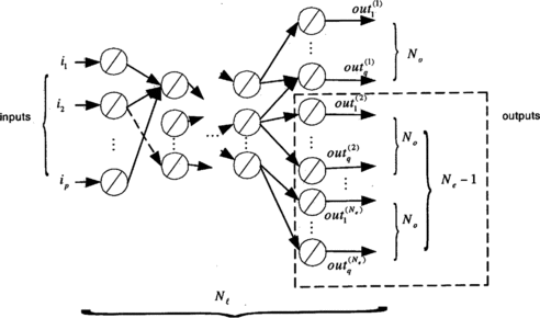
Note that the number of network outputs is increased N _e times from the original neural network, leading to the possibility of selecting which ones of them are used later. Hence, these rules define a multi-model neural network which includes all the sets of estimation algorithms, while the switching logic acts as an intelligent supervisor deciding the set of weights and/or the set of outputs that will be used for control purposes at each time instant. In such an easy way, the multi-model structure can be integrated together with conventional neural network-based controllers in order to obtain more general ANN-based multi-model structures. The general multi-model neural network scheme is displayed in Figure 7.

FIGURE 7 General multi-model ANN scheme.

Simulation Example for the ANN Representation

In this section, a simulation example containing two estimation algorithms and training rule (9) for the ANN displayed in Figure 6 is presented. The switching logic is assumed to respect a minimum residence number of samples given by N _r  = 2 between successive switchings between estimation algorithms in order to guarantee closed-loop stability (Ibeas et al. 2003). The switching law and the controller design (based on a model following pole placement algorithm) are described with detail in Ibeas et al. (2003). The discrete plant and reference model are described, respectively, by the parameter vectors:

while the estimators are initialized with the following estimated parameter vectors (or network weights):

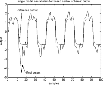
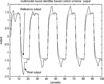
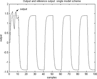
It is taken ε = 0.001 and α = 1. The input signal is a unity square wave with a 20 sample period. The performance index to decide switches is given by Equation (6) with λ = 0.95, β₂ = 1, and β₃ = 0. This choice for the parameters β indicates that the switching process only takes into account the identification error in order to choose the estimator which will parameterize the adaptive controller. The single adaptive control scheme is initialized with the first estimator. The following simulations comparing both the single estimation ANN and the multi-estimation one are obtained.

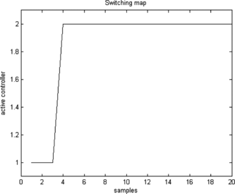
It can be concluded that a transient response improvement might be achieved by a using a multi-estimation scheme (see Figures 8 and 9). The transient overshot is less in the multi-estimation scheme than in the single-based one, while the real plant output tends to the desired output more smoothly in the multi-estimation case than in the single-based one as well. Also, note that the system improves its behavior by using the best weight set at each time (respecting the residence time constraint). The switching map c _k illustrating the switching process between both sets of weights (estimated parameter vectors) is shown in Figure 10. The proposed ANN integrates in a unique structure the complete set of estimation models running in parallel and the updating equations for the weights, whose role is represented by the estimated parameter vectors of a classic multi-estimation scheme. Thus, a multi-model ANN has been designed from a previously designed single model-based one in an easy way and applied to a concrete problem.

FIGURE 8 Single model-based output.

FIGURE 9 Multi-model-based neural controller.

FIGURE 10 Switching map for the multi-model ANN.

ANN Description of the Architecture of the Multi-estimation Control Scheme

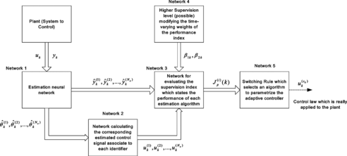
In this section, an ANN description of the architecture of the complete multi-estimation control scheme is stated. The key idea that develops the description is that ANN can be used to approximate (generate) any continuous nonlinear function (Fausett 1998). In particular, ANN will be able to generate the control signals and the supervision indexes that evaluate the identification performance of each estimation algorithm. Hence, we can describe the complete scheme by using a set of interconnected neural networks as displayed in Figure 11.

FIGURE 11 Description of the complete control scheme using neural networks.

The scheme is composed of the following networks:

	Network 1 (identification neural network). The aim of this network is to identify the parameters of the plant using the measurements of the output and the input to the plant y k , u k , respectively (obtained online for all time instants), in order to then use the estimated parameter values to calculate the control law by using the certainty equivalence principle. This set of estimation algorithms may be implemented either by N e independent identification neural networks running in parallel (which means that there is no information crossing between them despite all of them use the same input/output measurements to update their corresponding vectors), or by the complete ANN proposed in the previous section, where the evolution of some parameters modify the evolution of the remaining ones since all of them are trained together in a unique network. The entire network is trained by comparing the estimated output with the real plant output. Furthermore, it is not necessary to define the weights of the neural network as being the plant parameter vectors. The proposed architecture is applicable to any adaptive neural network controller, where the information that transmits the identification network to the next one is the network weights and/or outputs.
	Network 2 (estimated control signals network). Once the identification neural network has supplied the set of estimated parameter vectors and estimated outputs (in general its weights and outputs), a new ANN is used to calculate the potential control input corresponding to each estimated parameter vector. This step is necessary since the performance index may include a term weighting the change in the control signal due to switching. If the performance index were chosen without this term, this network would be removed from the presented scheme. This network may also be organized as composed by a number of individual ANNs working in parallel or by a unique one calculating all potential control signals in parallel. Since this network is disposed to calculate the potential pole-placement based control signals, it is not necessary to train it since it is basically used for calculation purposes.
	Network 3 (performance index calculation). Then the performance index can be calculated by using the estimated plant outputs and the estimated potential control inputs. Note that the performance index (6) includes a sum of these values over a window of previous samples. Hence, it would be necessary to include a battery of delays in the ANN first layer to hold the previous values of the estimated plant outputs and estimated plant parameter vectors. The length of this battery is the size of the supervision window H. Also, the performance index (6) involves a set of weights which act to modify the relative contribution of each addend to the global index. These weights could be supervised by alternative supervision algorithms as well (see, for instance, Ibeas and de la Sen [2004]).
	Network 4 (network for supervising the weights of the performance index). The workings of the supervision algorithm are based on heuristic rules and dynamically modify the value of the weighting factors according the evolution of the system through time. If the values of the weighting factors were constant, then this network implementing the supervision could be removed from the scheme leading to a simpler one.
	Network 5 (switching rule implementation). Finally, the switching rule selects one of the estimators to parameterize the adaptive controller using the values provided by the performance index, or in other words, it selects the estimated control signal that will be effectively applied to the plant.

Thus, note that the system architecture can be implemented by using an ANN technology. The system can be simplified by removing the corresponding networks associated with different supervision levels in the overall scheme. Moreover, it has been considered that the identification neural network can be divided into N _e independent neural networks, each one implementing one identification algorithm, while it being possible to possess a number of estimation algorithms running in parallel with mutual cross information. If we detect that an estimation algorithm is working better than the other ones, then we can aim the rest of them in the direction of the estimated parameter vector that is working in a better way. The following coupled (with mutual cross information between the estimation algorithms which compose the parallel scheme) multi-estimation algorithm is proposed.

Coupled Multi-estimation Scheme

The key idea that allows to define a coupled estimation algorithm lies on the fact that when the system detects that a concrete estimation algorithm leads to a better behavior than the others, then the scheme makes the remaining estimators evolve in the direction of the former. Thus, the following algorithm is proposed:

Algorithm 2. (Coupled identification algorithms)

	for k > 0 do
	if (k - lastSwitchingSample) < (residenceTime) then // the residence time constraint is not fulfilled
	for i = 1, 2,…, N e do // Update estimated parameter vectors according to the standard algorithm
	end_for
	else
	for i = 1, 2,…, N e do
	if then(ε > 0, fixed by the designer)
	else
	end_if
	end_for
	end_if
	end_for,

where the gain (which may be constant through time) is chosen to satisfy , with δ > 0 (fixed and finite) being selected by the designer while the maximum bound (finite of infinite) is determined by the stability and asymptotic properties of the standard least-squares algorithm obtained from the Lyapunov theory (Aström and Wittenmark 1995).

In the case when , the upper bound , defined in the same way, goes to infinity and no condition over the system gain value is stated since δ is finite. In practice, this condition means that the contribution of the new term to the dynamics of the estimation algorithm is small enough to maintain the asymptotic and stability properties of the original one. Note that the modification rule is only applied after the minimum residence time constraint is fulfilled. Therefore, the best estimation algorithm is known when the residence time constraint is respected. While in the other situation, we do not know which one is the best and thus the standard least squares algorithm has to be used. The following example illustrates the workings of this algorithm in a case study.

Case Study

Consider the following (unknown for control purposes) plant:

There are thirty estimation algorithms running in parallel initialized by:

for i = 1, 2,…, 30 while the covariance matrix is initialized by for all i. The control law is pole-placement based (Aström and Wittenmark 1995), with the control reference model:

where U _m (z), Y _m (z) are the z-transforms of the reference input and the model output sequences. Furthermore, a tracking performance index is proposed in order to compare the performances of the different schemes:

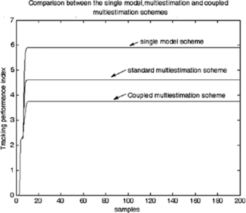
This index is a measure of the accumulated deviation of the real closed-loop output from the reference one, which gives an idea of the transient behavior of the scheme. The single model-based adaptive controller is initialized by the first estimator, while the parameters of the standard multi-estimation scheme are λ = 0.95 and β₁ = 0.95;β₂ = 0.05 in the supervision index (6). The coupled estimation algorithm works with a constant value of for all i and all k. The reference input is a sine wave of amplitude ±1 and angular frequency of ω = 2πrad/s.

In can be concluded that the coupled estimation algorithm may improve the closed-loop response of the control scheme, reducing the mean deviation of the real output from the reference one as the performance index reveals in Figure 12.

FIGURE 12 Comparison between the independent and coupled estimation algorithms.

GENETIC ALGORITHMS

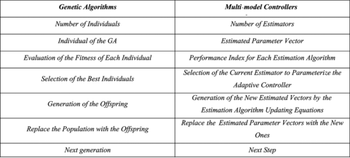
Genetic algorithms are used usually as optimization tools in complex problems (Abdennour 2004; Wetter and Wright 2004; Jamshidi et al. 2003). However, they have been applied recently to the intelligent control of dynamic processes (Mwembeshi et al. 2004). In this section, a genetic algorithm representation for multi-estimation-based control schemes is given. The key idea is to use the natural selection and the genetics to obtain, at each generation, more accurate solutions to an original problem (Beyers 1998). The multi-estimation-based adaptive control architecture has a great similarity with the structure and operation process of a genetic algorithm as Figure 13 illustrates.

FIGURE 13 Parallelism between multi-model controllers and genetic algorithms.

Thus, typical operators in the genetic algorithm context, namely, selection, cross-over, and mutation, have an adaptive counterpart in this context. The mutation operation is used in the sequel to select the estimated plant parameter vectors, which have an improved robustness property in comparison to the remaining estimators. The role of the cross over operator is represented by the estimation algorithm, while the selection operator is represented by the estimation algorithm selection policy (switching rule). Note that since a set of N _e estimation algorithms integrate the parallel multi-estimation scheme, it is obvious the usefulness of selecting the subset of them that better fits the identification performance to run the multi-estimation scheme with them while removing the rest, leading to worst behavior from the scheme. Hence, the mutation operation, typical in GA processes, can be applied to our problem in the following concrete way. At each time instant, mutate randomly the set of estimated parameter vectors to obtain a set of perturbed estimated parameter vectors . This new set is obtained by summing a Gaussian random perturbation with zero mean, variance unity, and maximum amplitude A to each component of the estimated plant parameter vector. The amplitude of the mutation is expressed as a % of the values of the original estimates vector:

where is the jth component of the vector, while (prefixed, finite, and selected by the designer as a very small positive number) is a bound which makes the definition wellposed. These perturbed estimated plant parameter vectors are then used to calculate a perturbed estimated plant output through the equations:

Thus, the perturbed estimated plant output can be compared with the unperturbed estimated plant one over a certain time interval to evaluate the robustness quality of each estimator. The proposed performance index is given by:

with β₁ + β₂ + β₃ = 1, β₁, β₂, β₃ ≥ 0. Note that the inverse of the index (6) has been considered in this case since a larger value for reveals a worse behavior of the corresponding estimator, while the GA philosophy states that the chromosomes quality function must be increasing with quality. Thus, the estimator selected to parameterize the adaptive controller, once the residence time constraint has been fulfilled, is the one associated to the maximum performance index (which is equivalent to select the estimator with the minimum value of the indexes). A penalty term about the identification robustness quality of each estimator has been incorporated to the original supervisory index (6) to obtain the proposed genetic index (12). Note that the robustness test is performed over a window of N samples size. The inclusion of this term is adequate when the plant is operating in a noisy environment. Thus, the deviation of the perturbed plant estimated outputs from the estimated unperturbed ones can be interpreted as a measure of the robustness property of the corresponding estimator and included in the criteria for switching between estimators.

Genetic Robustness Refinement

Moreover, the number of estimation algorithms can be decreased through time in order to reduce the computational cost of the algorithm. Thus, the number of estimation algorithms running in parallel can be pruned according to the following algorithm.

Algorithm 3. (Prune of estimation algorithms from the multi-estimation parallel scheme)

	{N e0, ΔN e  > 0, N eThreshold , N test  ≠ N r are selected by the designer}
	N e (0) ← N e0, k lastTest  ← 0
	or k > 0 do
	if k = k lastTest  + N test then
	if N e (k) > N eThreshold then
	Ne (k) ← Ne (k − 1) −)Δ Ne
	klastTest ← k
	else
	Ne (k) ← Ne (k − 1)
	end_if
	else
	Ne (k)← Ne (k − 1)
	end_if
	end_for ,

where χ represents a permutation of the N _e (k) estimation algorithms. When the residence number of samples for the prune algorithm N _test is fulfilled, then the estimators are ordered in a decreasing sequence according to the value of their supervision indexes . Then ΔN _e estimators with the minimum values of are pruned from the estimation process at regular time instants t = kT N _test (T being the sampling period), where k is a positive integer number, until the number of estimators reaches a minimum threshold of estimates N _eThreshold , when the prune process is stopped. After such a process, the system is only able to switch between the remaining estimators. The main usefulness of the scheme relies on reducing the computational cost of the multi-estimation scheme (in memory requirements basically), removing those estimators with the worst performance index. As it is typical in intelligent control (de la Sen et al. 2004; de la Sen and Almansa 2002), both supervisors have been designed to act with a different rate over the system. This choice avoids conflictive decisions between both supervisors. The following simulation example illustrates the workings of the proposed schemes. The simulation compares the workings of a single model-based adaptive control scheme, the classical multi-model-based adaptive control scheme for which β₃ = 0, and the genetic algorithm approach in both schemes. The first one in which the number of estimators remains constant through time and the second one in which the number of estimators reduces as time grows through a genetic prune process.

Simulation Example

Suppose that the plant input and output were affected by a Gaussian random perturbation with zero mean, unity variance, and a maximum amplitude of 4% of the original plant input and output signals. To generate the perturbed plant vectors , a Gaussian random perturbation is added to the estimated vectors as well. This test over the robustness quality of each estimator is used in the verification step, when the plant is working under the effect of a noise which will be simulated as a Gaussian random perturbation independent from the one used to define the perturbed plant outputs. In order to make a statistically meaningful interpretation of the proposed schemes, each scheme has been simulated 40 times affected by the random noise, and then the results have been averaged. The performance index (10) is used to compare the performance of all the schemes while the value of this index is averaged 40 times. The example is concerned with the same plant as in previous sections and the same reference model. There are 30 estimators running in parallel, while the single model-based adaptive control is initialized by the first one. The estimators are initialized by:

for i = 1, 2,…, 30. The amplitude of the test perturbation is A=5%. N _e0 = 30, ΔN _e  = 2, N _eThreshold  = 4, and N _test  = 6 samples. For the standard multi-estimation scheme, β₁ = 0.85;β₂ = 0.15;andβ₃ = 0. While for the robust schemes β₁ = 0.85;β₂ = 0.05;andβ₃ = 0.1. λ = 0.95 in all cases in (6). The results are presented in Figure 14.

FIGURE 14 Comparison between the single model-based adaptive control and the multi-estimation schemes.

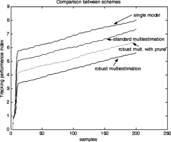
It can be concluded that multi-estimation based-techniques may improve the transient response of the adaptive system via a convenient parameterization of the adaptive controller through time. Thus, the performance index (10) is smaller for the multi-estimation schemes than for the single model-based one. Furthermore, the robustness term of the performance index (11) allows to improve the behavior of the standard multi-estimation scheme in the presence of noise as Figure 14 reveals for the performance index (12) for the robust multi-estimation scheme with a constant number of estimation algorithms. Also, if a prune over the multi-estimation scheme is performed, then the scheme improves its behavior in comparison to the single model-based one, but it gets worse in comparison to the original genetic algorithm one, which incorporates robustness issues. However, in this case, some computations are pruned, which reduces the memory storage requirements with the drawback that a worse behavior than the original complete genetic algorithm scheme, which maintains the number of estimators constant through time, is achieved.

FUZZY LOGIC APPROACH

In this section, a fuzzy logic approach for multi-estimation-based control schemes is given. As it is well known, fuzzy set theory is a generalization of the classical set theory (Tilli 1992; Alonso-Quesada et al. 2004; Ibeas and de la Sen 2004; de la Sen and Almansa 2002, Ibeas et al. 2004; de la Sen et al. 2003; Liutkevicius 2003; Wang and Qing 2004; Mwembeshi et al. 2003; Liutkevicius 2003; Wang and Qing 2004; Mwembeshi et al. 2003; Wetter and Wright 2004; Feng 2004). It allows a class of objects with a continuum grade of membership to a set. Such a set is characterized by a membership (characteristic) function which assigns to each object its grade of membership to the set ranging from one to zero. The classic set theory operations are extended to the fuzzy case as well. Inference relations over fuzzy set objects define the so-called fuzzy logic. Fuzzy logic, together with artificial neural networks and genetic algorithms, completes the set of techniques used in intelligent control (Liutkevicius 2003; Wang and Qing 2004; Mwembeshi et al. 2004; Wetter and Wright 2004; Feng 2004; Etxebarria and de la Sen 1996; Melin and Castillo 2003). 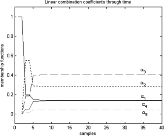Thus, in the multi-estimation scheme presented previously, an estimated parameter vector is chosen from a set of parameter estimated vectors to parameterize the adaptive controller at each sampling time. However, instead of choosing a single estimated vector, it is also possible to define a combined estimated vector as:

where 0 ≤ α _{i, k}  ≤ 1, 1 ≤ i ≤ N _e and ∀ k ≥ 0. The linear combination (13) is convex in the sense that , ∀ k ≥ 0. Definition (13) implies that at each time instant, the combined estimated parameter vector belongs to the convex hull (Co) (lbeas and de la Sen 2004) of the individual estimated parameter vectors and then:

In the standard cases (considered here and in Ibeas et al. [2003]), only one coefficient α _{i, k} is different to zero and equal to unity while the rest of the parameters take a value of zero. However, it is also possible to let each coefficient α _{i, k} take a value running from zero to unity. Then, we can interpret each one as a membership function of the combined estimated vector _k to the corresponding estimation algorithm with vector . According to a recent work (Alonso Quesada et al. 2004), the following membership function is proposed in order to clarify the interpretation:

where the symbolizes the performance indexes defined in (6), and used for evaluating the quality of each estimation scheme potentially parameterizing the adaptive controller. Also, note that a larger performance index for an estimation algorithm leads to a less membership function of the combined estimated vector to the corresponding estimation algorithm. Also, the updating of the membership functions must respect a minimum residence time in order to guarantee the closed-loop stability, (Ibeas and de la Sen 2004). Thus, the following updating rule is proposed for interpretation purposes:

where N _r  > 0 is the residence number of samples with α _{i, 0} being an arbitrary initialisation. This kind of combined multi-estimation control scheme has been applied recently to the nonlinear adaptive control of robotic manipulators as well Ibeas and de la sen 2004). Figure 15 illustrates the diagram of the proposed multi-estimation scheme.

FIGURE 15 Fuzzy logic inspired multi-estimation scheme.

This approach to multi-estimation schemes has been used in robotics (Ibeas and de la Sen 2004) to define a combined estimated plant parameter vector. In addition, combining different estimation algorithms to obtain a new one to parameterize the adaptive controller has been broadly used in the multi-model adaptive control literature (see, for instance, Cezaylirli and Ciliz [2004]), where the coefficients of the linear combination were updated by using a metric-based approach. Nevertheless, it has never been pointed out the relationship between this and the fuzzy logic/fuzzy set theory. Therefore, it may be possible to define fuzzy rules for determining online the values of the coefficients of the linear combination weights in order to achieve a predefined closed-loop behavior, opening a wide variety of applications of the fuzzy logic to multi-model control.

Simulation Example

The following simulations comparing the single model-based and the fuzzy logic-based multi-estimation schemes show the usefulness of the proposed scheme. The plant, the input signal, and the performance index used in (15) are the same as in the ANN example. The estimation algorithm is of standard least squares type for all the estimation algorithms. The residence time is two samples. There are five estimators running in parallel and initialized by:

with for i = 1, 2,…, 5. The initial values for the membership functions are:

and they are updated by Equation (15), respecting the residence time constraint (with β₂ = β₃ = 0). The single adaptive control scheme is initialized by the first estimator. The simulations in Figures 16, 17, and 18 are obtained.

FIGURE 16 Classical adaptive control scheme.

FIGURE 17 Combined adaptive control scheme.

FIGURE 18 Membership functions α _{i, k} .

It is apparent from Figures 16-18 that the fuzzy logic-based combined multi-estimation scheme improves the transient response of the adaptive system. The transient over peak is reduced due to switching to a more convenient parameterization of the adaptive controller through the convex linear combination of the estimators of the multi-estimation scheme, according to the updating rule (15). The transient response improvement is achieved once the residence number of samples constraint is fulfilled since the updating rule is not allowed to modify the weight values until then.

CONCLUSIONS

In this paper, an artificial intelligence representation of multi-estimation-based controllers has been developed. A graph theory-based representation of the switching process between the different estimation schemes is introduced. This representation allows to describe in a formal way the structure and workings of the switching process, providing a concise description of the switching logic. A neural network interpretation of multi-model based-controllers has been given, while a method for generating multi-model-based artificial neural network controllers from previously designed single model ones has been proposed. The ANN description of the overall system allows to implement the complete scheme using ANN technology. Also, a coupled estimation algorithm has been proposed in order to take opportunity of the information contained in the set of estimators running in parallel. The estimator selected to parameterize the adaptive controller guides the evolution of the remaining ones to its location. Moreover, the genetic algorithm and fuzzy logic-based approaches have been given to represent multi-estimation-based schemes. These artificial intelligence techniques have suggested new ideas to be incorporated into the classic multi-model controllers. The genetic algorithm approach has inspired a robustness test over the set of estimation algorithms which allows the improvement of the workings of the multi-estimation scheme in noisy environments. Also, the fuzzy logic approach suggests a way to combine the estimation algorithms in order to build an estimated parameter vector which parameterizes the adaptive controller. Some simulation examples show the usefulness of the proposed multi-estimation structures for improving the transient response of adaptive systems.

Acknowledgments

The authors are grateful to MEC and to the UPV-EHU by its partial support of this work through projects DPI 2003-00164, UPV 9/UPV 00I06.I06-15263/2003. Also, the authors are grateful to reviewers who have helped to improve the final version of this manuscript and to Professor J. M. Tarela whose comments about genetic algorithms helped to improve the paper. A. I. is very grateful to MECD by its support of this work through the FPU grant P2002-2727.

REFERENCES

- Abdennour , A. 2004 . Multi-objetive optimal tuning of power plant controls using genetic algorithms . Control and Intelligent Systems 32 ( 2 ): 80 – 88 . [CSA]
- Alonso-Quesada , S. , M. De la Sen , A. Bilbao-Guillerna , and A. Ibeas . 2004. A semiempirical identification method by using a multiestimation technique via reduced-order nominal models. In: Proceedings of the 2004 American Control Conference, pages 4372–4377.
- Aström , K. J. and B. Wittenmark , 1995 . Adaptive Control, Addison-Wesley Publishing Company. , 2nd Edition .
- Beyers , H. G. 1998 . The Theory of Evolution Strategies . Berlin: Springer-Verlag .
- Cezayirli , A. and K. Ciliz . Multiple model based adaptive control of a DC motor under load changes , Proc. Of the International Conference on Mechatronics 2004 , Istanbul, 1–3, June, 2004 .
- Chang , M. H. and E. J. Davison . 1999 . Adaptive switching control of LTI MIMO systems using a family of controllers approach . Automatica 35 : 453 – 465 . [CSA] [CROSSREF]
- Chartrand , G. and L. Lesniak 1979 . Graphs and Digraphs, , Second Edition . Pacific Grove , CA : The Wadsworth and Brooks/Cole .
- Chen , L. and K. S. Narendra . 2001 . Nonlinear adaptive control using neural networks and multiple models . Automatica 37 ( 8 ): 1245 – 1255 . [CSA] [CROSSREF]
- Ruan , D. , ed. 1997 . Intelligent Hybrid Systems, Fuzzy Logic, Neural Networks and Genetic Algorithms . Boston : Kluwer .
- de la Sen , M. and A. Almansa . 2002 . Adaptive stable control of manipulators with improved adaptation transients by using on-line supervision of the free parameters of the adaptation algorithm and sampling rate . Informatica Lithuanian Academy of Sciences 13 ( 3 ): 345 – 368 . [CSA]
- de la Sen , M. , S. Alonso-Quesada , A. Bilbao-Guillerna , and A. J. Garrido . 2003 . A supervised multiestimation scheme for discrete adaptive control which guarantees robust closed-loop stability . Int. Math. J. 3 ( 9 ): 907 – 937 . [CSA]
- de la Sen , M. , J. J. Miñambres , A. J. Garrido , A. Almansa , and J. C. Soto . 2004 . Basic theoretical results for expert systems. Application to the supervision of adaptation transients in planar robots . Artificial Intelligence 152 ( 2 ): 173 – 211 . [CSA] [CROSSREF]
- Diestel , R. 2000 . Graph Theory. , Second Edition . New York : Springer-Verlag .
- Etxebarria , V. 1994 . Adaptive control of discrete systems using neural networks . IEE Proc. Contr. Theory and Appl. Part D. 141 ( 4 ): 209 – 215 . [CSA] [CROSSREF]
- Etxebarria , V. and M. De La Sen . 1996 . An approach to adaptive neural control of robot manipulators . International Journal of System Science 27 ( 11 ): 1143 – 1152 . [CSA]
- Fausett , L. V. 1998 . Fundamentals of Neural Networks . Englewood Cliffs , NJ : Prentice Hall .
- Feng , G. 2004 . Stability Analysis of discrete-time fuzzy dynamic systems based on piecewise Lyapunov functions . IEEE Transactions on Fuzzy Systems 12 ( 1 ): 22 – 28 . [CSA] [CROSSREF]
- Gregorcic , G. , A. Mullane , and G. Lightbody . 2001 . Simulink implementation of adaptive control and multiple model network control . In: Proceedings of the Nordic Matlab Conference , pages 167 – 173 , October .
- Hocherman-Frommer , J. , S. R. Kulkarni , and P. J. Ramadge . 1998 . Controller switching based on output prediction errors . IEEE Transactions on Automatic Control 43 ( 5 ): 596 – 607 . [CSA] [CROSSREF]
- Ibeas , A. and M. de la Sen . 2004 . Intelligent control of robotic manipulators based on a multiestimation scheme . In Proceedings of the IASTED International Conference Artificial Intelligence and Applications , pages 694 – 699 .
- Ibeas , A. , M. de la Sen , and S. Alonso-Quesada . 2003 . Adaptive stabilization of discrete linear systems via a multiestimation scheme . Int. Math. J. 3 ( 4 ): 381 – 407 . [CSA]
- Ibeas , A. , M. de la Sen , and S. Alonso-Quesada . 2004 . Intelligent control of discrete linear systems based on a supervised adaptive multiestimation scheme . Journal of Intelligent and Robotic Systems 40 ( 4 ): 359 – 411 . [CSA] [CROSSREF]
- Jamshidi , M. , L. dos Santos Coelho , R. A. Krohling , and P. J. Flemming . 2003 . Robust Control Systems with Genetic Algorithms . Boca Raton , FL : CRC Press .
- Liutkevicius , R. 2003 . Coupled adaptive fuzzy control of nonlinear, time-varying plant . Informatica Lithuanian Academy of Sciences 14 ( 3 ): 323 – 336 . [CSA]
- Melin , P. and O. Castillo . 2003 . Adaptive intelligent control of aircraft systems with a hybrid approach combining neural networks, fuzzy logic and fractal theory . Applied Soft Computing 3 ( 4 ): 353 – 362 . [CSA] [CROSSREF]
- Mosca , E. and T. Agnoloni . 2001 . Inference of candidate loop perfomance and data filtering for switching supervisory control . Automatica 37 : 527 – 534 . [CSA] [CROSSREF]
- Mwembeshi , M. M. , C. A. Kent , and S. Salhi . 2004 . A genetic algorithm based approach to intelligent modelling and control of pH in reactors . Computers & Chemical Engineering 28 ( 9 ): 1743 – 1757 . [INFOTRIEVE] [CSA] [CROSSREF]
- Narendra , K. S. and J. Balakrishnan . 1994. Improving transient response of adaptive control systems using multiple models and switching. IEEE Transactions on Automatic Control 39(9):1861–1866. [CSA] [CROSSREF]
- Narendra , K. S. and J. Balakrishnan . 1997 . Adaptive control using multiple models . IEEE Transactions on Automatic Control 42 ( 2 ): 171 – 187 . [CSA] [CROSSREF]
- Sun , Z. 2004 . A robust stabilizing law for switched linear systems . Int. J. Control 77 ( 4 ): 389 – 398 . [CSA] [CROSSREF]
- Sun , Z. and S. S. Ge . 2003 . Dynamic output feedback stabilization of a class of switched linear systems . IEEE Trans. On Circuits and Systems 50 ( 8 ): 1111 – 1115 . [CSA] [CROSSREF]
- Tilli , T. 1992 . Fuzzy Logic . Munich : Franzis-Verlag .
- VanDoren V. , ed. 2003 . Techniques for Adaptive Control . Amsterdam : Elsevier Science .
- Wang , J. and M. Qing . 2004 . An output tracking control strategy for unknown nonlinear systems . Applied Artificial Intelligence 18 ( 1 ): 1 – 16 . [CSA]
- Wetter , M. and J. Wright . 2004 . A comparison of deterministic and probabilistic optimization algorithms for nonsmooth simulation-based optimization . Building and Environment 39 ( 8 ): 989 – 999 . [CSA] [CROSSREF]