APPLICATION OF HIERARCHICAL NEURAL FUZZY MODELS TO MODELING AND CONTROL OF A BIOPROCESS

Abstract

Hierarchical structures have been introduced in the literature to deal with the dimensionality problem, which is the main drawback to the application of neural networks and fuzzy models to modeling and control of large-scale systems. In the present work, hierarchical neural fuzzy (HNF) models are reviewed, focusing on the model-based control of a biotechnological process. The model considered here consists of a set of neural fuzzy systems connected in cascade and is used in the modeling of an industrial plant for ethyl alcohol (ethanol) production. Based on the HNF model of the process, a nonlinear model predictive controller (HNF-MPC) is designed and applied to control the process. The performance of the HNF-MPC is illustrated within servo and regulatory scenarios.

In recent years, model predictive control (MPC) algorithms (Soeterboek 1992; Qin and Badgwell 1997; Camacho and Bordens 1994; Morari and Lee 1999) have successfully been applied to control of complex industrial processes. In most of these applications the controller is implemented using a linear model of the process under interest. Industrial processes, however, are usually nonlinear and, in these cases, the use of MPCs based on linear models may lead to poor closed-loop performances.

The development of more efficient mathematical models of nonlinear processes has been sustained on the successive advances in the capacity for memory storage and processing of the latest computational devices. In this context, two important classes of nonlinear models are the feedforward architectures of neural networks (Haykin 1999) and fuzzy systems (Yager and Filev 1994) especially because these models are universal approximators, i.e., they can approximate to arbitrary accuracy any continuous mapping defined on a compact (closed and bounded) domain. However, due to their generic structures, both neural and fuzzy models usually require the estimation of a large number of parameters. Generally, the number of parameters and data needed to provide a desired degree of accuracy increases exponentially with the dimension of the input space of the mapping to be approximated. This is the well-known problem called “curse of dimensionality” (Kosko 1997; Haykin 1999). In order to get around this problem, Raju et al. (1991) proposed a hierarchical structure of fuzzy systems in which a set of lower-dimensional subsystems are connected in cascade. In this structure the number of fuzzy rules increases linearly (instead of exponentially) with the dimension of the input space, thus being of particular interest to applications involving large-scale processes.

Mathematical results have shown that hierarchical fuzzy models can also be constructed as universal approximators (Wang 1998; Chen and Wang 2000; Campello and Amaral 2002), despite their reduced structure. Nevertheless, the application of these models in real-world problems requires efficient numerical approaches for the estimation of their free design parameters from a finite input-output data set measured from a system to be modeled. Wang (1999) proposed the use of neuro-computing techniques for this purpose, but only models with three input variables were considered. A similar approach based on a generic formulation suited for models with any number of inputs was proposed by Campello and Amaral (2000), who developed a hierarchical neural fuzzy system composed of simplified fuzzy relational subsystems which are, under certain conditions, completely equivalent to radial basis function (RBF) neural networks (Broomhead and Lowe 1988). This approach is considered in the present paper in the context of an industrial application.

The industrial application considered here is concerned with a biotechnological process. Biotechnology has become increasingly important in the activities of contemporary society as a “clean” and safe technology when compared to traditional chemical processes. Moreover, it provides extremely useful and valuable products in several industrial areas (pharmaceutical, foods, fuels, etc.). Biotechnological processes are characterized by their complex dynamics, such as inverse response, dead time, and strong nonlinearities, especially because the main driving force of these processes is derived from microorganisms (cells) that are very sensitive to any environmental variations in the fermentation broth (e.g., temperature, substrate concentration, and pH, among others). For these reasons, modeling, simulation, and control of those systems are still a relevant and timely research theme.

The present paper focuses on the modeling and control of a typical large-scale industrial plant to produce ethanol from sugar cane syrup. The process operational conditions are those typically found in the Brazilian industrial distilleries. A hierarchical neural fuzzy (HNF) model of this process is estimated and validated using data for those typical conditions. Based on this model, a constrained nonlinear predictive controller is designed to control the process. The controller makes use of the successive quadratic programming (SQP) algorithm to solve the optimal control problem at each sampling interval and performs properly even in the presence of strong disturbances acting on the plant.

SIMPLIFIED FUZZY RELATIONAL STRUCTURE

Consider a multi-input/single-output (MISO) system given by y = F(x ₁,…, x _n ), where F is a nonlinear operator which maps the inputs x _i (i = 1,…, n) into the output y. This system can be modeled using a simplified relational structure (Oliveira and Lemos 1998), given by the following equation:

where ŷ is the model output, Ω(m × 1) is the parameter vector, and Ψ(m × 1) is the fuzzy input vector. Vector Ψ is given by the Kronecker Product (⊗) (Graham 1981) of the individual fuzzy inputs, i.e.,

The inputs X _i (i = 1,…, n) are derived from the nonfuzzy inputs x _i as follows:

where is the jth fuzzy set of the ith input variable (with c _i fuzzy sets).

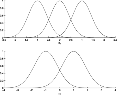
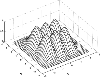
It is possible to demonstrate that the fuzzy model given by the equations presented is completely equivalent to an RBF neural network with Gaussian activation functions whenever Gaussian fuzzy sets are used (see the Appendix). The analogy between these models is illustrated in Figures 1 and 2 for a two-dimensional input space. Figure 1 shows Gaussian fuzzy sets defined on the domains of the input variables x ₁ and x ₂ of a simplified fuzzy structure. Figure 2 shows the activation functions of the equivalent RBF network. It can be noted that the fuzzy sets are the projections of the multivariate activation functions onto the unidimensional spaces of the input variables.

FIGURE 1 Fuzzy sets of a fuzzy model with two inputs: (above); (below).

FIGURE 2 Activation functions (6 neurons) of the equivalent RBF neural network.

Model Structure

The model given by Equations (1), (2), and (3) follows the conventional structure of fuzzy models (FM) and feedforward neural networks (NN) shown in Figure 3-a. The main problem with this structure is discussed in the sequel.

FIGURE 3 (a) Nonhierarchical model. (b) Relationship between the number of inputs, n, and fuzzy rules/neurons, m.

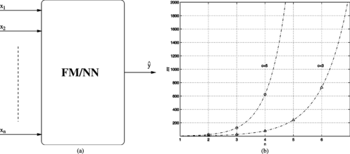
Consider, for simplicity and without loss of generality, that c _i  = c for i = 1,…, n in (3). Then, it can be seen from Equation (2) that the number of elements of both vectors Ψ and Ω in (1) is given by m = c ⁿ . This is the number of fuzzy rules associated with the model or, alternatively, the number of neurons in the equivalent RBF network. This is also the number of parameters to be estimated (synaptic weights in the RBF networks) if the fuzzy sets/activation functions are kept constant. On the other hand, if the centers and widths of the fuzzy sets/activation functions can be varied, then the number of parameters to be estimated becomes p = c ⁿ  + 2nc. Note that the approximation capability of the model depends directly on c.

The exponential relationship between the number of inputs, n, and the number of fuzzy rules/neurons, m, is shown in Figure 3-b for typical values of c. This figure illustrates the dimensionality problem in nonhierarchical models, i.e., the increase in the number of fuzzy rules/neurons needed to cover the input space with given “density” as an exponential function of the number of inputs n. Hierarchical models are presented in the next section as an alternative to avoid this dimensionality problem.

HIERARCHICAL NEURAL FUZZY (HNF) MODELS

As outlined previously, an approach to overcome the dimensionality problem of the conventional (nonhierarchical) models is the hierarchical structure shown in Figure 4-a, where n − 1 submodels (processing blocks) with two-dimensional input spaces are connected in cascade. Although submodels with different numbers of inputs could also be used, the configuration with just two inputs will be considered hereafter because it leads to the most parsimonious model (Raju et al. 1991). In this case, the number of fuzzy rules/neurons in each submodel is c ². Consequently, the total number of fuzzy rules/neurons in the model is m = (n − 1)c ²(n ≥ 2). This is also the number of parameters to be estimated if the fuzzy sets/activation functions are kept constant. Otherwise, the number of free design parameters becomes p = (n − 1)c ² + 2nc + 2(n − 2)c = (n − 1)c ² + 4(n − 1)c.

FIGURE 4 (a) HNF Model. (b) Relationship between the number of inputs, n, and fuzzy rules/neurons, m.

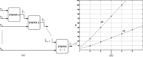
The relationship between the number of inputs, n, and the number of fuzzy rules/neurons, m, is displayed in Figure 4-b for typical values of c. This figure shows that the rate of growth in the number of fuzzy rules/neurons as a function of the number of inputs is constant (for n ≥ 2). This is a significant advantage in comparison with the behavior of the nonhierarchical structure shown in Figure 3-b.

Formulation

Based on the formulation presented previously, the equations that describe the model shown in Figure 4-a are:

where X _(·) and Y _(·) are the fuzzy sets associated with the inputs x _(·) and hidden (intermediate) outputs ŷ _(·), respectively, and is the parameter vector of the ith submodel. When Gaussian fuzzy sets are used, for instance, it follows that:

where (or ) and are the center and the width of the lth fuzzy set associated with the jth input x _j (or hth hidden output ŷ _h ), respectively. The formulation presented describes the hierarchical model as a kind of layered fuzzy neural network. The identification of this model by means of data-driven optimization algorithms is discussed in the sequel.

Optimization Problem

Consider a set of N input/output data pairs, i.e., , measured from a system to be modeled. Then, a hierarchical model of the system can be estimated by solving the following optimization problem:

where Γ denotes the set of all free design parameters of the model. Problem (10) can be solved using nonlinear optimization techniques (Bazaraa et al. 1993), such as the conjugate gradient algorithm of Fletcher and Reeves. This algorithm is particularly well suited to large-scale problems since it does not demand the computation of any Hessian matrix or its inverse. In addition, it ensures the convergence of the optimization procedure with second-order rate.

The optimization techniques mentioned require the computation of the gradient vector of the cost function J with respect to the set of parameters Γ. The set Γ related to the hierarchical models considered here is composed of the parameter vectors Ω_(·) in Equation (4), as well as the centers (θ_(·) and φ_(·)) and widths (σ_(·) and ϕ_(·)) of the fuzzy sets in Equations (8) and (9). The derivatives of J in (10) with respect to these parameters can be computed by applying the chain rule to Equations (4) through (9). The corresponding analytical equations can be found in Campello and Amaral (2000).

Parameter Initialization

The input and output variables should be normalized within a certain interval, such as [−1, 1], in order to avoid numerical problems during the model optimization procedure. Then, the fuzzy sets associated with a given input or hidden output can be initialized homogeneously within the normalization interval, which means equally spaced centers and widths equal to the distance between two consecutive centers. The fuzzy sets of the input variables could be initialized optionally using fuzzy clustering techniques (Babuška 1998).

The parameter vectors Ω_(·) should be initialized randomly with zero mean and absolute values small enough so that the initial values of the hidden outputs belong (at least approximately) to the normalization interval.

HNF MODEL-BASED PREDICTIVE CONTROL

Controllers of particular interest to chemical and biochemical processes are the so-called model predictive controllers (MPC) (Clarke 1994). The aim of these controllers is to select a set of future control actions in order to minimize an objective function typically given by:

where λ is a suppression factor, i.e., a tuning parameter that penalizes the control actions, Δu is the increment on the manipulated variable, N ₁ is the initial horizon, N _y is the prediction horizon, N _u is the control horizon, w is the reference trajectory (or setpoint), and ŷ _k+i is the model prediction of the controlled output at the future sampling instant k + i. The term d _k is a correction term, defined as d _k  = y _k  − ŷ _k (Clarke 1994), where y _k is the measured output at the current sampling instant k and ŷ _k is the respective model prediction (calculated at the previous sampling instant k − 1).

The optimization algorithm computes the increments Δu so as to minimize the objective function (11). The future control actions are then derived from the optimal control increments as:

It is important to remark that only the first N _u control actions are optimized, whereas the remaining ones are kept constant, i.e.:

The optimization problem is also subject to the following additional constraints:

where y _min and y _max, u _min and u _max, and Δu _min and Δu _max are lower and upper bounds for y, u, and Δu, respectively. In addition, the receding horizon strategy is adopted (Soeterboek 1992; Camacho and Bordons 1999), in which only the first control action u _k is implemented and the optimization problem is solved again at the subsequent sampling instant.

Particularly, owing to the characteristics of the nonlinear equations that govern the HNF model predictions, the optimization problem presented is nonconvex. Accordingly, an appropriate methodology is required to solve it. In this paper, the successive quadratic programming (SQP) algorithm is adopted (Edgar and Himmelblau 1981).

INDUSTRIAL PROCESS FOR ETHANOL PRODUCTION

Introduction

The Brazilian alcoholic fermentation processes arose from the production of the sugar cane liquor (aguardiente). Later, these processes were applied to production of ethanol from molasses obtained from the sugar production plants. In the 1980s, the Brazilian federal government's “pro-alcohol” program created an incentive for the use of ethanol as an alternative fuel in automobiles. As a consequence, there was an increase in research focusing on improving the productivity and yield of these processes. Current research concentrates on the optimization of the continuous operation of the processes.

As stated previously, an industrial plant for the production of ethanol is considered in the present work. Because of difficulties encountered when working directly with the plant in operating mode, especially owing to the high costs involved when interrupting its operation for tests, it has been chosen to work with a simulator whose kinetic parameters have already been validated in the real plant (Andrietta 1994; Andrietta and Maugeri 1994). This validated simulator models the biochemical process by means of a set of phenomenological nonlinear ordinary differential equations and presents excellent agreement with actual data measured from the industrial plant under interest.

Plant Description

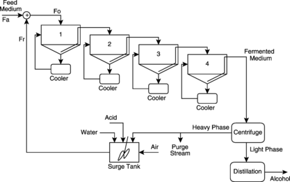
The fermentative process for ethanol production is illustrated in Figure 5. The system is a typical large-scale industrial process composed of four tank reactors (fermenters) arranged in series and operated with cell recycling to produce ethanol from sugar cane syrup. Each reactor has an external system of heat exchangers with independent control loops (PI controllers) whose objective is to maintain the constant temperature of the reactants (fermentation broth) at an ideal level for the fermentation process. The setpoint for the temperature was optimized by Andrietta (1994) to maximize the efficiency of the reactions (conversion) of the industrial plant.

FIGURE 5 Schematic illustration of the industrial plant for ethanol production.

The process is fed with a mixture composed of sugars (total reducing sugars - TRS) as well as sources of nitrogen and mineral salts, called feed medium. The feed medium is converted into ethanol by a fermentation process carried out using the yeast Saccharomyces cerevisae. A set of centrifuges splits the outlet fermented medium, which is formed of a mixture of water, CO₂, sugars, microorganisms (30–45 kg/m³ of cells), and alcohol, into two phases. The heavy phase contains most of the cells (160–200 kg/m³), whereas the light phase contains at most 3 kg/m³ of cells and is 9–12% alcohol. The light phase is sent to the distillation unit, where the alcohol is extracted. The heavy phase is submitted to an acid treatment and dilution before being recycled into the first reactor. The recycling procedure is important because the generation of new microorganism colonies is an expensive and time-consuming process.

The industrial process for ethanol production is highly nonlinear. The main nonlinearities arise from the behavior of the microorganisms. Increasing the feed medium flow rate, for example, causes the TRS concentration inside the tanks to increase. Under this condition, the ethanol production from the biological conversion of the sugar tends to increase. However, an excessive amount of sugar, which exceeds the microorganisms' processing capacity, will not be converted into ethanol (substrate inhibition phenomenon). This excess of sugar will appear in the final product, thus characterizing a drop in the conversion efficiency as well as a waste of raw material and energy. All of these factors influence the dynamics and the efficiency of the fermentation process. More details on this process can be found in (Andrietta 1994), and a set of trials illustrating its nonlinear behavior is presented in Dechechi (1998).

The fundamental objective of the study of the fermentative process for ethanol production is to generate models and controllers so as to maximize its efficiency. In the present context, this means to regulate the substrate concentration in the outlet of the fourth tank, which is directly related to the economic feasibility of the process.

Input, Output, and Disturbances Variables

The input, output, and disturbance variables of the process are:

	Feed Medium Flow Rate (F a [m3/h]): This is the manipulated input variable. The universe of discourse of this variable is the interval [50,150]. This interval is conservative in terms of the economic and operational viability of the plant. It represents the upper and lower bounds for the substrate feed flow and comprises the limitations related to valve operation and tank volumes as well.
	Recycle Rate (t r [dimensionless]): This variable relates the feed medium flow rate, F a , with the cell recycle flow rate (F r [m3/h]) and, accordingly, with the actual inlet feed flow rate in the first tank (F 0 [m3/h]), as shown in Figure 5. This relationship is given by F 0 = F a  + F r  = F a /(1 − t r ). Thus, a recycle rate of 0.3 implies F a  = 0.7F 0 and F r  = 0.3F 0. This is the pre-optimized industrial operation value for the plant under interest. This nominal value can eventually be changed slightly by a plant worker to fix problems in the microorganism colony. In this case, this variable is considered to be a measurable disturbance.
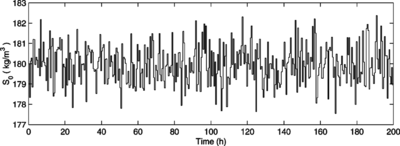
	TRS Concentration in the Feed Medium (S 0 [kg/m3]): The nominal value of this variable under real operational conditions is 180 kg/m3. However, since it depends on the sugar cane used, it is important to take into account possible disturbances around this value. In this case, this variable becomes a measurable disturbance.

The output variable of interest (according to the control objective discussed previously) is TRS Concentration in the Outlet of the Fourth Tank (S ₄ [kg/m³]), where the outlet product of the fourth tank is the fermented medium (see Figure 5).

HIERARCHICAL NEURAL FUZZY MODELING OF THE ETHANOL PRODUCTION PROCESS

Data Generation and Sampling

The strategy of dealing with a validated simulator of the actual process makes it possible to generate identification data as desired. Thus, a representative data set containing the input and output signals of the process related to 1000 hours (≈40days) of its simulated operation was generated. In these data, the manipulated variable F _a is a sequence of steps, each of which with period of 10h (long enough so that the process can nearly reach the steady state) and random amplitude uniformly distributed within the operational interval [50, 150]. The inputs t _r and S ₀ are also sequences of steps. However, they were given Gaussian distributions for the amplitudes and periods of 25 h and 50 h, respectively, so that they can express the underlying statistical characteristics of the measurable disturbances, i.e., their greatest probability of taking the respective nominal values or their neighboring values most of the time. To accomplish this, the Gaussian probability distribution functions were centered on the nominal values of t _r and S ₀, i.e., S₀ = 180kg/m³ and t _r  = 0.3. The standard deviations were set as 1/6 of the respective operational intervals ¹ in such a way that the amplitudes of the randomly generated steps belong to these intervals with a probability of approximately 99%.

The data set was sampled using the traditional procedure in which the sampling period T is derived in such a way that N _T  = T _s /T ≈ 4 to 10 (Aström and Wittenmark 1997) where T _s is the rise time of the process and N _T is the number of data samples during this time. The rise time of the industrial process considered in the present work is roughly between 2 h and 3 h, which implies T ≈ [12 min, 45 min]. In addition, the sampling period must be a multiple of 15 min, which is the typical interval between samples of the chromatograph (the device used for measuring the TRS concentrations involved in the process). For the sake of the considerations mentioned, a value of T = 30 min was selected. This value is large enough to avoid numerical problems and gives rise to a set of 2000 discrete-time input-output data pairs: the first 1000 pairs (≈20 days of plant operation) intended for the estimation of a hierarchical model of the process and the remaining ones intended for the validation of this model.

Structure Selection

Structure here refers to three distinct concepts: i) the regressors, i.e., the relevant past terms of the input and output variables of the process to be used as inputs into the model; ii) the hierarchical order of the model inputs; and iii) the internal structural settings of the model itself.

The most significant regressors of the process are known to be F _a (k − 1), F _a (k − 2), S ₀(k − 1), t _r (k − 1), and S ₄(k − 1) (Meleiro 2002). Their hierarchical order as inputs into the model, though not critical,was selected using a priori knowledge about the basic behavior of the process. More specifically, a set of dynamic response experiments performed in the ethanol production plant was considered (Dechechi 1998). These experiments point out that, as expected, the manipulated variable F _a is the most important input, having the highest influence on the dynamic response of the process. Hence, the corresponding regressors were placed on the first hierarchical levels, i.e., x ₁ and x ₂ (see Figure 4-a), since the number of parameters (degrees of freedom) that relates these inputs and the model output is the largest among all the others. The experiments cited also show that the nonlinearities associated with the disturbance S ₀ are stronger than those associated with the disturbance t _r . Hence, the hierarchical order of the former was set greater than that of the latter. Thus, an adequate hierarchical order for the regressors as inputs into the model was selected as x ₁ = F _a (k − 1), x ₂ = F _a (k − 2), x ₃ = S ₀(k − 1), x ₄ = t _r (k − 1), and x ₅ = S ₄(k − 1).

The internal structure of the model was defined as described previously. A small number of fuzzy sets (c = 2) was adopted to prevent an excessive number p of unknown parameters to be estimated. This number of fuzzy sets is capable of providing adequate results in the present application, as shown in the next section.

It is important to remark that all the structural settings specified could optionally be included into a genetic algorithm (Bäck et al. 2000) to be determined in an automated manner together with the remaining parameters of the model. This strategy would, however, increase the computational requirements of the model estimation procedure.

Model Estimation and Validation

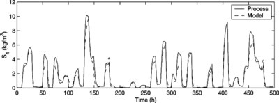
The HNF model was trained using the estimation data set throughout 1000 iterations of the Fletcher and Reeves algorithm, when the optimization procedure could no longer significantly improve the model and no overfitting had yet occurred. The synthetic data simulation of the resulting model using the validation data is shown in Figure 6. The term “synthetic data” denotes a recursive simulation in which the model does not rely on past values of the system output to predict its future behavior. In this sense, this simulation is much more stringent than the well-known one-step-ahead prediction.

FIGURE 6 Synthetic data simulation of the HNF model: validation data set.

The mean squared error (MSE) between the outputs of the process and the model is MSE = 0.3384. This result shows that the HNF model adequately represents the nonlinear dynamics of the process, especially considering the long-range prediction horizon comprised in the simulation.

PREDICTIVE CONTROL OF THE ETHANOL PRODUCTION PROCESS

The HNF model derived in the previous section is used as the internal nonlinear model for the predictive controller described previously, named hereafter the hierarchical neural fuzzy model predictive controller (HNF-MPC). The operational constraints on the manipulated and controlled variables of the process are:

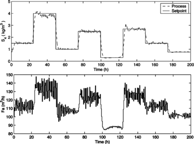
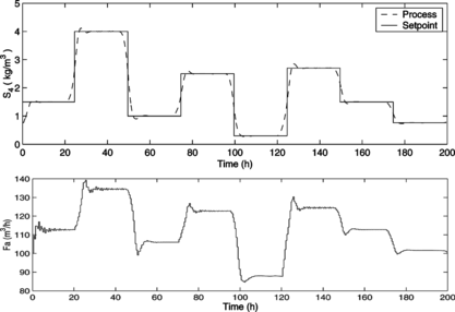
As discussed previously, the disturbances acting on the process are the TRS concentration in the feed medium, S ₀, and the recycle rate, t _r . It can be shown that these disturbances strongly influence the process dynamics (Dechechi 1998). Initially, however, it is assumed that there are no disturbances acting on the process, i.e., S ₀ and t _r are kept constant at their nominal values (S ₀ = 180kg/m³ and t _r  = 0.3). Under this assumption, the controller is tuned as N ₁ = 1, N _y = 10, N _u = 2 and λ = 0.005. The closed-loop simulation of the ethanol production process is presented in Figure 7, which shows that the designed HNF-MPC is able to control this nonlinear process with good performance.

FIGURE 7 Closed-loop simulation of the HNF-MPC in servo scenario: reference and process output (above); manipulated input (below).

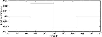
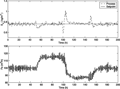
In what follows, the presence of disturbances acting on the process is taken into account. In the first experiment, S ₀ is still considered to be constant, whereas t _r is varied as shown in Figure 8. The closed-loop simulation of the process is shown in Figure 9, which shows that the controller is capable of rejecting the disturbance.

FIGURE 8 Changes in the recycle rate.

FIGURE 9 Closed-loop simulation of the HNF-MPC in regulatory scenario: reference and process output (above); manipulated input (below).

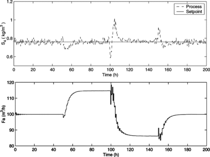
In the following experiments, the previous simulations are repeated assuming that S ₀ is a stochastic disturbance as shown in Figure 10. Figures 11 and 12 refer to the closed-loop response of the process in servo and regulatory scenarios, respectively. As expected, the disturbance worsened the performance of the control scheme, although the controller is still capable of controlling the process properly. It is very important to remark that the controller has not been retuned to deal with the disturbances so that its performance under adverse situations can be evaluated.

FIGURE 10 TRS concentration in the feed medium as a stochastic disturbance.

FIGURE 11 Closed-loop simulation of the HNF-MPC in servo scenario, taking into account stochastic disturbances in S ₀: reference and process output (above); manipulated input (below).

FIGURE 12 Closed-loop simulation of the HNF-MPC in servo scenario, taking into account stochastic disturbances in S ₀ and t _r : reference and process output (above); manipulated input (below).

CONCLUSIONS

In the present work a hierarchical neural fuzzy (HNF) model has been used for the identification of a complex biotechnological process for ethyl alcohol (ethanol) production. Simulations have shown that this model can adequately represent the process dynamics with a reduced number of free design parameters, even over long-range horizon predictions. A nonlinear predictive controller based on the HNF model of the process (HNF-MPC) has been designed and tested. This controller comprises constraints on manipulated and controlled variables, and makes use of the successive quadratic programming (SQP) algorithm to solve the optimal control problem at each sampling interval. The HNF-MPC has successfully been applied to control of the substrate concentration in the outlet stream of the process in both servo and regulatory scenarios, thus allowing an effective and economically feasible operation of the industrial plant.

Notes

1. S ₀ ∈ [170, 190] and t _r  ∈ [0.27, 0.33].

APPENDIX

Equation (1) can be rewritten explicitly as

where and denote elements of Ψ and Ω, respectively, in such a way that and . Each element can be written from Equations (2) and (3) as

Whenever Gaussian fuzzy sets are used, Equation (21) can be rewritten from (8) as

Since the product of n unidimensional Gaussian functions is an n-dimensional Gaussian function, Equation (22) results in

where

From Equations (20) and (23), it can be seen that the model output is given by a weighted sum of multivariate Gaussian functions, which is precisely the architecture of an RBF neural network (Haykin 1999).

REFERENCES

- Andrietta , S. R. 1994 . Modeling, Simulation and Control of Industrial-Scale Processes for Continuous Alcoholic Fermentation . Ph.D. thesis, State University of Campinas – UNICAMP, Campinas/SP/Brazil (in Portuguese) .
- Andrietta , S. R. and F. Maugeri . 1994 . Optimum design of a continuous fermentation unit of an industrial plant for alcohol production . In: Advances in Bioprocess Engineering , eds. E. Galindo and O. T. Ramírez , 47 – 52 . Kluwer Academic Publishers .
- Åström , K. J. and Wittenmark , B. 1997 . Computer-Controlled Systems. , Third edition , Prentice Hall .
- Babuška , R. 1998 . Fuzzy Modeling for Control . Kluwer Academic Publishers .
- Bäck , T. D. B. Fogel , and Z. Michalewicz . editors . 2000 . Evolutionary Computation 1: Basic Algorithms and Operators/Evolutionary Computation 2: Advanced Algorithms and Operators . Institute of Physics Publishing .
- Bazaraa , M. S. , Sherali , H. D. , and Shetty , C. M. 1993 . Nonlinear Programming: Theory and Algorithms, , Second edition . John Wiley & Sons .
- Broomhead , D. S. and D. Lowe . 1988 . Multivariate functional interpolation and adaptive networks . Complex Systems 2 : 321 – 355 . [CSA]
- Camacho , E. F. and Bordons , C. 1999 . Model Predictive Control . Springer-Verlag .
- Campello , R. J. G. B. and Amaral , W. C. 2000 . Optimization of hierarchical neural fuzzy models . In Proceedings of the IEEE-INNS-ENNS International Joint Conference on Neural Networks , Como/Italy .
- Campello , R. J. G. B. and Amaral , W. C. 2002 . Hierarchical fuzzy relational models: Linguistic interpretation and universal approximation . In Proceedings of the 11th IEEE Internat. Conference on Fuzzy Systems , Honolulu , Hawaii, USA .
- Chen , W. and Wang , L.-X. 2000 . A note on universal approximation by hierarchical fuzzy systems . Information Sciences 123 : 241 – 248 . [CSA] [CROSSREF]
- Clarke , D. W. , editor . 1994 . Advances in Model Based Predictive Control . Oxford University Press .
- Dechechi , E. C. 1998 . Modern Adaptive Predictive Control “Multivariate DMC,” Ph.D. thesis, State University of Campinas – UNICAMP, Campinas/SP/Brazil (in Portuguese) .
- Edgar , T. F. and Himmelblau , D. M. 1988 . Optimization of Chemical Processes . McGraw-Hill .
- Graham , A. 1981 . Kronecker Products and Matrix Calculus . Ellis Horwood Ltd .
- Haykin , S. 1999 . Neural Networks: A Comprehensive Foundation, , Second edition . Prentice Hall .
- Kosko , B. 1997 . Fuzzy Engineering . Prentice Hall .
- Meleiro , L. A. C. 2002 . Design and Application of Linear, Neural, and Fuzzy Model-Based Controllers , Ph.D. thesis, State University of Campinas – UNICAMP, Campinas/SP/Brazil (in Portuguese) .
- Morari , M. and Lee , J. H. 1999 . Model Predictive Control: Past, Present and Future . Computers and Chemical Engineering 23 : 667 – 682 . [CSA] [CROSSREF]
- Oliveira , J. V. and Lemos , J. M. 1998 . Improving adaptive fuzzy control performance by speeding up identification: Application to an electric furnace . Journal of Intelligent and Fuzzy Systems 6 : 297 – 314 . [CSA]
- Qin , S. J. and Badgwell , T. A. 1997 . An overview of industrial model predictive control technology . In: Chemical Process Control , eds. J. C. Kantor , C. E. Garcia , and B. Carnahan , volume 93 of AIChE Symposium Series , 232 – 256 .
- Raju , G. U. , J. Zhou , and R. A. Kisner . 1991 . Hierarchical fuzzy control . Int. J. Control 1201 – 1216 . [CSA]
- Soeterboek , R. 1992 . Predictive Control – A Unified Approach . Prentice Hall .
- Wang , L.-X. 1998 . Universal approximation by hierarchical fuzzy systems . Fuzzy Sets and Systems 93 : 223 – 230 . [CSA] [CROSSREF]
- Wang , L.-X. 1999 . Analysis and design of hierarchical fuzzy systems . IEEE Trans. Fuzzy Systems 7 : 617 – 624 . [CSA] [CROSSREF]
- Yager , R. R. and Filev , D. P. 1994 . Essentials of fuzzy modeling and control . John Wiley & Sons .
APPENDIX
Equation (Equation1) can be rewritten explicitly as