A BEHAVIORAL AGENT MODEL FOR SYNTHESIZING VEGETATION DISTRIBUTION PATTERNS ON 3D TERRAINS

Abstract

Vegetations, similar to other organisms, persist on terrains based on niches of their abiotic and biotic environments. Agent-based models of vegetation have demonstrated that, via the process of macro self-organization, are capable of forming forests and undergrowth by means of their behavior and the resources available in the ecosystem. In order to more accurately synthesize their collective behavior, a set of rules encompassing basic vegetation behavior were defined to enable realistic patterns to be formed locally via interaction and extra-locally via emergence in accord with their preferences in various controlled environments. Furthermore, the use of botanical parameters fine-tuned and regulated via simple rules could, in the near future, become a potential model for determining large-scale spatial and temporal distribution of dominant vegetation species, enhancing traditional methods and visualization in studies related to forest dynamics and research in landscape reconstruction.

View correction statement:

ERRATUM

Emergence—a phenomenon that occurs in living systems through the local interaction of organisms—has in recent years been studied and used extensively in the artificial life (alife) community and new trends of artificial intelligence (AI) (Kim and Cho 2006). The widespread popularity in studies related to the concept of emergence is attributed to its effectiveness and efficiency in problem-solving, and the comparatively simple modelling techniques utilized. It is found that the inherent properties in nature for self-reproduction, self-assembly, and self-organization necessarily embodies certain principles that could be used in a variety of domains with great effectiveness. By emulating these principles, scientists in various domains are now able to gain new perspectives in their fields and to resolve challenges that were unattainable using traditional methodologies. One of the modelling practices is “the bottom-up approach, which is based on parallel, distributed networks of relatively simple, low-level agents that simultaneously interact with each other” (Kim and Cho 2006). According to Resnick (1994b), one of the main characteristics of these low-level decentralized agents is that they are “organized without an organizer” and “coordinated without a coordinator.” This self-organization reflects the mechanisms of all adaptive and complex systems (Lewin 1993; Waldrop 1993; Mainzer 1994; Holland 1995; Stacey 1996). Indeed, “The most promising approaches to modelling complex systems like life or intelligence are those which have dispensed with the notion of a centralised global controller, and have focused instead on mechanisms for the distributed control of behavior” (Langton 1989).

Emergence as defined by Stacey (1996) is “the production of global patterns of behavior by agents in a complex system interacting according to their own local rules of behavior, without intending the global patterns of behavior that come about.” Agents in complex systems interact by the internal simple rules of behavior that accompanied them. Examples of biologically inspired agents with simple rules are extensive. Those studied (von Neumann and Burks 1966; Berlekamp, Conway, and Guy 1982; Wolfram 2002) and applied (Reynolds 1987; Huth and Wissel 1992; Niwa 1994; Bonabeau and Theraulaz 2000; Gajardo, Moreira, and Goles 2002; Kunz and Hemelnijk 2003) include the flocking and schooling behavior of birds and fishes and swarm intelligence in social insects. From the examples given, it is observed that as long as we can find the principle rules inherent in these systems, any variables of the physical system can be digitized and its characteristics synthesized for study or for problem-solving.

The benefits of synthesizing vegetation behavior using an agent-based approach are constrained only by time. If the model is well defined, landscapes from the past, the present, and even the future can be simulated, and forest formation in relation to climate changes is predictable for benefiting studies related to landscape archaeology, landscape architecture, and forest planning.

A survey of literature related to alife and vegetation modelling yielded only a handful of articles (Hanan 1995; Prusinkiewicz, Hammel, Me˘ch, and Hanan 1995; Mech and Prusinkiewiez 1996) of which only several (Damer, Marcelo, and Revi 1998; Lange, Thies, Kastner-Maresch, Dorwald, Kim, and Hauhs 1998) are useful for simulation in large landscapes. This is, of course, to be expected as the science of alife is relatively new for addressing this particular direction of research. A related model (Damer 1998), whilst claiming to exhibit properties of growth, decay, and energy transfer reminiscent of a simple ecosystem, presents a somewhat primitive solution from an alife perspective since it does not support plant growth or interaction between plants and the environment (Luck and Aylett 2000). A closer model is Lange et al.'s (1998) growth simulator using Tree Response to Acidification in Groundwater in C + + (TRAGIC +). Lange et al.'s method for tree growth is derived from local competition for energy and nutrients with only two input fluxes—energy and a growth-limiting nutrient. The model presented in this research contrasts with Lange's approach in the inclusion of a generic model of customizable vegetation lifecycle that corresponds to different vegetation types (trees, shrubs, herbs, grass, etc.) with seasonal differences (evergreen, deciduous). Competitions amongst plants for resources are determined by their canopy, density of leaves, height, vegetation types, and tolerance towards crowd spaces. Furthermore, the adaptable ecological factors and resources (sunlight, temperature, carbon dioxide, altitude, soil, hydrology, etc.) other than the two input fluxes described in Lange et al.'s model are important determinants for vegetation communities in an ecosystem (Grime, Hodgson, and Hunt 1988) and should be taken into account.

Other methods of plant modelling related to GIS are available (e.g., Davis and Goetz 1990; Spikins 1999, 2000; Gearey and Chapman 2005). However, some studies suggest that GIS has limitations with regards to cognitive representations, temporal analysis, three-dimensional analysis, and the accuracy of the represented model (Cross 2003; Ebert and Singer 2004; Fyfe 2005). Furthermore, models used for simulating the distribution patterns of plants did not utilize to the fullest the techniques that are currently available in alife. For example, a prominent work in landscape archaeological reconstruction (Spikins 2000) uses a top-down approach as evident by its nonagent-based technique. The program runs through two nested “loops,” the outer cycled through each date or period for whichthe model was being run; the second goes through the mapping of each different possible woodland type allocating a dominant type for each region of the terrain described with base maps. This if-else-then technique characterizes many GIS-based techniques. In a study (Cairns 2001), a comparison of three more advanced methods have shown that the accuracy of these methods varies depending on a specific situation, and that there may not be a single best predictive method. This may be due to the limitations of the approach in the predictive modelling.

The present research aims to fill up the lack in previous modelling techniques by leveraging the concept of emergence and the principles associated with artificial life. This necessitates the study of the life cycle of vegetation in order to extract, generalize, and synthesize its behaviour as internal rules in decentralized agents for the purpose of formulating a potential model for determining large-scale spatial and temporal distribution of dominant vegetation species.

VEGETATION MODELLING

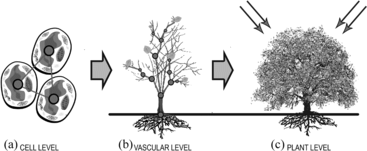
According to the bottom-up methodology in alife, an approach for modelling vegetation could begin from the cellular level (Figure 1a), with interacting cells forming the smaller components of a tree, and the smaller components forming the vascular systems (Figure 1b) whose structure eventually completes the tree. Another way is to model the vascular structure of a tree (Figure 1b) with its root and shoot system interacting with itself, the environment, and other plants to form a tree that is limited by its pattern architecture (species). Each of these approaches may be useful for certain studies; however, considering the limitations of computing resources and the specific problem domains we are attempting to solve, in order to determine vegetation dispersal patterns on large terrains, modelling vegetation as complete entities (Figure 1c) that respond to ecological factors, availability of resources, and threats from competition and the environment may be a more feasible approach.

Figure 1 A bottom-up approach for simulating vegetation. (A) Cell level; (B) vascular level; (C) plant level.

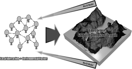
Learning from examples in living systems, we could perceive landscapes as large organisms composed of many decentralized entities (species of vegetation), which collectively form and replenish the larger systems (landscapes) by forming patterns of forests and colonies by relying on the availability of resources and the suitability of the ecology on the ecosystem (Figure 2). In accordance with the concept of emergence, the local interaction of these vegetative communities, in addition to ecological variables, should appropriately synthesize the formation of vegetation communities on niches of each species' ecology on terrains, if the behavioral rules of these agents are well-defined.

Figure 2 Perception of a landscape as a large organism composed of vegetation as its entities.

ARTIFICIAL LIFE-BASED VEGETATION MODEL

Modelling the different species of vegetation requires a thorough understanding of plant life in order to generalize its life cycle, properties, and behaviors for the purpose of configuring this information into states and rules suitable in an environment that is entirely described by data structures and algorithms. A mapping of real botanical parameters to variables within each agent is also necessary for synthesizing their behaviors. With a small amount of “fine tuning” of the properties acquired from studies related to botany (Tansley 1965; Grime, Hodgson, and Hunt 1988; Ingrouille 1995), individual plants can be modelled to a level of accuracy sufficient for solving problems in vegetation dispersal patterns. Knowledge in the category listed below is necessary for modelling plant life:

	the life cycle of different plants
	the preferences of plants
	the growth type of plants (evergreen, deciduous, etc.)
	the tolerance or adaptability of different plants to different environmental conditions
	the reproductive life cycle
	the conditions suitable for seed germination.

Studies have been conducted and experiments carried out in order to determine the most appropriate way of using alife concepts to synthesize vegetation. The following algorithms are formulated for synthesizing plant life:

	plants reproduce in their assigned season.
	seeds are dispersed in different directions and dispersal agents are simulated by dispersing the seeds much further away.
	seeds have a period of dormancy before suitable environmental conditions cause them to germinate; seeds expire if they are not germinated within an assigned period of time.
	Plant tolerance/adaptation to ecosystem factors is based on an upper, ideal, and lower value. Different plants have different values.
	Plants compete for availability of sunlight, space, and nutrients based on environmental conditions and the sizes and shapes of competing plants.

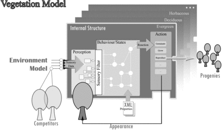
Figure 3 illustrates a generic model of vegetation used in this study. The agent-based plant possesses sensors for sensing ecological and seasonal changes, both reacting and adapting to variations based on properties and preferences, which includes seed germination and adaptability information of plants toward different environmental conditions. The alife-based vegetation germinates from a seed before beginning its life cycle of growth, adaptability, competition, reproduction, and death. The procedure of synthesizing vegetation into computational models of life necessitates the generalization and distillation of their behaviors into rules. The rules are defined in the subsections below.

Figure 3 A generic, agent-based vegetation model.

Plant Adaptability

Adaptation in vegetation denotes avoidance and tolerance to environmental hazards (Slatyer 1967; Bjorkman 1968; Chapin 1980; Clark and Ben Forado 1981; Fitter and Haw 1981; Solbrig 1981; Vitousek 1982; Crawley 1986). Adaptations of plants in botany-related studies have shown that over thousands of years, survival of plants in extreme environmental conditions may be countered via the development of physical characteristics that are tolerant to hazardous conditions. Adaptation of vegetation in this research uses Ch'ng's adaptability measure (Ch'ng 2007). Equation (1) shows an example:

where C is the current environmental condition or resource availability sensed by an agent, U and L refer to the upper and lower tolerance value of condition C, p is an ideal condition preferred by the plant, and b in the range [0, 1] defines the hardiness of the plant.

Rules for Nutrient Availability

The availability of nutrient is derived from three sources—condition of the soil, decaying components from living agents, and the decaying components from dead agents. The first is a global parameter that varies according to seasonal changes, and the latter two supplement the level of nutrients accessible to the local clustering of vegetation communities. Intensity of nutrients naturally increases around a higher number of vegetation clusters and from dead agents. The rule of nutrient accessibility and agent-based plant decay is defined as follows. Nutrients from decaying matter from an agent are accessed only if the agent has the following distance from another agent:

where i is an opponent agent with location, x _i and y _i . The location of the source agent is at x, y with radius r.

The level of nutrients from the decaying components of a living agent nearby is:

where c _i is the canopy of individual agent with leaf density d _i and radius r _i .

If a nearby agent has expired and is decaying, the nutrient generated by that plant is :

where g is the gradient generally [0.1, 0.5], s _i is the size of the agent at the time of death, t is the time-step from the virtual environment, and d is the rate of decay. The size of the virtual representation is set to decrease over time at the same rate of decay and affects competition for space.

Equation (5) is the effective nutrients received by the source agent:

where n is the number of living and decaying agents at proximity. i, an individual agent, can be either dead , or living, ·N ^global refers to the global nutrient level, which is set to approximate the inverse of the level of sunlight in Figure 4.

Figure 4 Monthly mean temperature and sunlight.

Rules for Competition

The competition of a plant is mainly from sunlight and space. The effective sunlight received by a plant is determined by its height, canopy, and density of leaves in relation to other plants. It is possible that a plant in the undergrowth receives no sunlight in a dense forest. A simple rule of competition for sunlight is:

The effective shade of a competitor agent is measured by:

where i is the individual opponent with location, x _i and y _i , canopy c _i , and leaf density d _i . The location of the source agent is at x _s , y _s with radius r _s .

The effective sunlight received by an agent under the shade of nearby intersecting agents is therefore:

where n is the number of agents in competition, i is an opponent, and L ∊ [0, 1] (Figure 4) is the sunlight received by the source agent if it is not under any canopy.

Certain plants are tolerant to crowded spaces whereas others are not. The competition for space among plants is dependent on their size, form, and distance. A plant's establishment in age and its size is advantageous to those that are smaller. Via observation of plant clusters, the rule for competition for space is:

The competitor agent occupies a space based on its size. The intensity of the competition between different agent and competitor sizes is modelled. Two formulas are used for determining the occupation of space—one for larger opponents and the other for opponents smaller or equal in size. The space occupied by a larger opponent is generated by the rule,

where λ, with the most effective range [0.25, 0.3], is the space used if the source agent is at size s, x _i is the size of the opponent. Experiments suggest the following values as most effective: For agent size s ≤ 10 meters, I = 5, w = 3. For agent size 10 > s < 25 meters, I = 5, w = 2. For agent size s > 25 meters, I = 10, w = 2.

The space occupied by a smaller opponent is generated by the rule

where λ, with the most effective range [0.25, 0.3], is the intensity of the use of space, x _i is size of the opponent, s is the size of the source agent. For agent size s ≤ 10 meters, I = 1. For agent size 10 > s < 25 meters, I = 5. For agent size s > 25 meters, I = 10.

The effective space occupied collectively by competitors is therefore

where C is the totality of the space occupied by opponent agents, n is the number of agents in competition, i is an opponent, and P _i is space occupied by an opponent.

MODELS OF SYNTHETIC ENVIRONMENT

The environment is a crucial factor in determining the physical conditions of living systems. The simulation environment for the synthesis of life and the task environment for distributed agents need to be well-defined. Quoting Herbert Simon in The Sciences of the Artificial (1997), Resnick (1994) stated that we should not underestimate the role of the environment in influencing and constraining behavior: “People often seem to think of the environment as something to be acted upon, not something to be interacted with. People tend to focus on the behaviors of individual objects, ignoring the environment that surrounds (and interacts with) the objects…a richer view of the environment is particularly important in thinking about decentralized and self-organizing systems.”

Synthesizing dispersal patterns of vegetation required knowing the environment in the target landscape in order to provide equal opportunities for plants suited to different habitat to thrive and compete in the following:

	The global environment conditions of the landscape—variable seasonal sunlight, temperature, moisture, nutrients, and carbon dioxide
	The local environment conditions affected by plants at proximity—effective sunlight, moisture, and availability of space, soil Ph, soil depth
	Temperature-altitudinal ratio
	Hydrology
	Ground and soil conditions—soil acidity, soil depth, ground texture, slope angle.

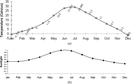
In the synthetic environment, the terrain is continuous and defined by 3D polygons. Experimental scenarios for studying the behaviors of agent-based vegetation using custom terrains for better control of the environment. Time is discreet and global bioclimatic parameters are derived from a monthly mean temperature, soil humidity, CO₂, and other important environmental conditions. For efficiency of simulation when dealing with large time-scales (hundreds to thousands of years), the use of month-time is logical in many systems (e.g. Fischlin and Bugmann 1994; Zimmerman and Kienast 1999; Bergengren, Thompson, Pollard, and Deconto 2001). Figure 4 shows two global ecological parameters—temperature in Celsius and sunlight measured in the range [0, 1].

Temperature is set to decrease proportionally at T = 0.6°C per 100 m. This temperature-altitudinal ratio is simulated with

where T _effective is the effective temperature, T is the ratio of decrease, E is the current altitude where a plant is at, and T _global is the seasonal global temperature defined in Figure 4.

Hydrology is defined with the range [0, 1]. The distribution and increase of moisture content of the soil is a continuous gradient to below the water surface so that water-resistant plants and plants tolerant to waterlogging can be synthesize, the rule for defining hydrology on a terrain is

where W _effective is the effective moisture level, M is the moisture level below the water surface, E is the current altitude where a plant is at, W _surface is the water surface, and g is the gradient.

Two models define the local environments such as the local effective sunlight, temperatures, ground, and soil conditions on the 3D terrain. In the first model, the local environments are affected by the presence of vegetation. Trees and large plants affect the sunlight received by the undergrowth which in turn affects its temperatures. The second model uses height fields for defining the four conditions of the soil and ground—soil acidity, soil depth, ground texture, and slope angle.

OBSERVATIONAL STUDY: ARTIFICIAL VEGETATION BEHAVIOR

Nonlinear simulations such as these require observational studies of individual agent behaviors and their collective responses to the environment. Observational studies will enable us to determine the credibility of the model in terms of correlations with naturally occurring phenomenon in the behaviors of biological plants. This section describes the simulation outcome of the model in a virtual environment.

Effects of Environmental Factors

Four species of agent-based plants (green, red, yellow, blue) were released into a simulated environment (Figure 5). The topology of the landscape increases in elevation towards the top of the screen. This implies that as we approach the top of the landscape, the temperature decreases proportionally. The sensing ability of the agents was limited to only temperature and elevation. Competition occurs in the occupation of available space between agents at proximity. At T3, each species begins producing offspring. T15 shows that certain agents and some of their offspring begin to die (turning white) as a result of competition and the environment. The global temperature were gradually increased in T34 and plants were observed to migrate north due to the simulated global warming. The simulation in T34 also showed a species (red) that cannot adapt to the environment, leaving no offspring. It finally exceeded its lifespan, resulting in the extinction of that species. T56 showed a condition known as the climax community, where the emerging patterns of species colonization have reached a stable condition.

Figure 5 Simulated global warming and its effects on agent-based plant species (plan-view).

In Figure 6, three species of plants each having a different adaptability trait were scattered on a landscape with hydrological influence—the higher regions of the terrain have less soil moisture content as compared to the lower regions of the landscape where water converged. T0 shows the initial placements of the species. At T8, the niches of each species have become obvious through the expiration of species unable to adapt to dry or wet soils. A stable condition can be seen in T12.

Figure 6 A scenario showing the preference of three agent-based plant species in a landscape with different levels of soil moisture content.

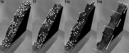
Figure 7 is a terrain with compressed elevation-temperature ratio where T = 10°C for Equation (11). This implies that at the two ends of the landscape elevation are the extreme conditions. Labels R, G, B are overlaid on the figures for clarity. The red species (R) are adaptable to hot temperatures as compared to the blue species (B), which adapts to extremes of cold. The green species (G) has a moderate adaptation. T0 is an initial random scattering of each species. T7, T10, and T16 show the developments of the species in their respective niche. T16 shows a clear separation of habitat.

Figure 7 A scenario showing the preference of theree agent-based plant species in a landscape with a compressed temperature-elevation ratio.

Competition for Space

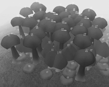
A landscape populated with three species of plants can be seen in Figure 8:

	Tall trees–intolerant to crowd
	Shrubs–possessing an intermediate adaptability to crowd
	Undergrowth–high adaptability to crowd.

Figure 8 Agent-based plant species competing for space.

In the scenario, the fitness of each agent (shown as “h:fitness”) varies as they are affected by competition from other agents with different sizes. Number of competing plants are shown as “c:competitors.” Trees, being intolerant of crowds, are the most affected species. Shrubs and the undergrowth did not show signs of vulnerability in this simulation.

Effects of Sunlight and Shade

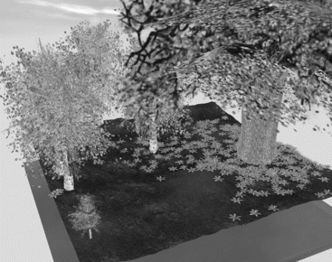
Figure 9 is a scenario where plant species clustered. The simulation demonstrates the effects of shade on certain species. Large trees were not affected as they do not have competitors. Most of the shrubs showed a level of fitness of “ < 0.01,” indicating their inability to adapt to shaded conditions. Figure 10 is a simulation with representations of three species of vegetation—oaks, birches, and ferns. The simulation demonstrates the effects of sunlight and shade on the fern species, which can be observed to grow only in the shade of the trees where the sunlight and temperature are milder. The preferences of the species are shown in the Appendix.

Figure 9 Effects of sunlight and shade on agent-based fern species.

Figure 10 Generic ground condition for illustrating the agent-based plant's adaptability.

Effects of Ground and Soil

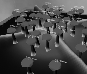
Figure 11 demonstrates the fitness and adaptability of one species of plant towards a generic soil condition. White represents the ideal condition. The increasingly darker areas represent uninhabitable regions. The fitness of plants (shown as “F:fitness”) are higher in the lighter regions of the landscape. In Figure 12, three conditions of the soil are established. White regions are the extreme condition of the soil. In Figure 12(a), white regions have the coarsest ground texture. The white regions in Figure 12(b) have the highest concentration of soil acidity. The white regions in Figure 12(c) depict the shallowest soils. In the simulation, the red species in 12(a), 12(b), and 12(c) have the highest population, demonstrating its adaptability to all levels of conditions.

Figure 11 Effects of ground and soil conditions on different species of agent-based plants.

Figure 12 An ecological simulation of the interaction between agent-based plants and their environment.

Collective Environmental Effects

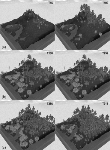
In the previous section, individual environmental effects have demonstrated the feasibility of the model described using the agent-based plant rules. This section demonstrates the collective effects of the environment described in the previous sections towards four species of agent-based vegetation—pine, birch, willow, and the hazel—which is set to arrive via migration at T150. The preferences of these species are shown in the Appendix.

The simulation showed the progression and colonization of each species in their respective niche. The population densities of species in certain regions depict the niches of that species' environment. In the simulation, the willow species appear to colonize around where water converged. Pine and hazel are the dominant species in the terrain, covering the majority of the landscape. Birches have the lowest population density and appeared only in the upper regions of the terrain.

DISCUSSIONS

The way different plants colonize a landscape possesses different characteristic patterns. Such patterns can be observed in abundance in nature. Ferns appear to cluster together in abundance around shady areas with lower temperatures and higher soil moisture content, and the growth of certain species of cactus is sparse in dry deserts. In a pine forest, the pine species are grouped together in sparse distances with undergrowth covered by shade-tolerant species. Willows are observed to grow near water sources. The environment plays an important role in the colony of plant species. In situations where there is a progressive gradual rise of the earth's surface temperature, such as global warming, plants unable to adapt or migrate at a speed necessary to survive will eventually die out.

In order to verify the agent-based vegetation's behavior, it is necessary to observe such patterns in the virtual environment. The agent-based experimental studies have demonstrated credible relationships between the artificial and the natural, all through the rules described in the methodology. In the first experiment where global warming is simulated, the agents appear to “move” towards regions where the environment is habitable. This is achieved by the dissemination of progenies. Agents unable to adapt eventually expires, and if no offspring is left, the particular species of agent becomes extinct. This also implies that the ecological niches of a certain species warrant a higher population density of that species (e.g., Figures 5–7, 10, and 12). For example, a clear distinction of each species' niche is shown in Figures 6 and 7. In the two experiments, the environments describe a gradual transition from two extreme conditions—Figure 6 on hydrology and Figure 7 on temperature. The experiments showed that, except for species with intermediate adaptability (green), which inhabit the intermediate and one of the extreme conditions, the other species thrived in their respective niches. The studies presented above also demonstrate a phenomenon observable in nature—ecotones and ecoclines—the local clustering of similar species over time due to reproduction and suitable ecology.

Knowledge and observations acquired from botany suggests that competition among plants occurs mainly in three directions—sunlight, space, and nutrients. Depending on the genotype of the agents (see Appendix), the simulations in Figures 8 and 9 suggest that different species have different adaptability towards crowded settings due to competition. The experiments showed that by using the rules of competition, plant competition can be simulated, that is, crowd-tolerant plants thrive on compact spaces, whereas crowd-intolerant plants are disadvantageous in terms of their growth and reproduction. The rules also suggest that smaller plants are at a disadvantage. However, in another scenario (Figure 10), instead of competition, the large tree became a catalyst for growth of a smaller species (ferns) due to its preference for decreased sunlight and local temperature variation.

For survival and reproduction in all the studies, but especially Figures 5 and 13 have shown that open spaces afford a better chance of continuation of that species as competition is at a minimum.

Figure 13 The position of the Shotton River Valley in the North Sea.

It is interesting to note that a set of simple rules described and experimented in the previous sections could simulate naturally occurring behaviors, particularly that of the plant. And that vegetation colonization of a virtual terrain via collective interaction between these plants and its immediate environment can be properly simulated. Through observations in nature and in the present research, implementing it has taught us that many systems can be reduced to a set of rules and behaviors using agent-based systems. Coupled with parameters acquired from related sciences, these systems can be simulated to a level of accuracy for solving real world problems. Looking into the future, we can imagine a system for solving problems in landscape reconstruction research such as in archaeology, geology, predictive modelling of the effects of climate change on forest dynamics, and perhaps even evolution of the plant species in advanced future developments.

CONCLUSION AND FUTURE WORK

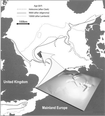
The model presented in this article has provided a way for synthesizing generic plant species. The emerging patterns formed by the local interaction between plant species and its response to global and local environment witnessed in the experiments demonstrate the feasibility of the model in many related applications where vegetation is needed. Currently, in collaboration with the Institute of Archaeology and Antiquity (IAA) and the Hewlett-Packard Visual and Spatial Technology Centre (HP VISTA), at the University of Birmingham, UK, the model is being refined as a tool for research on a submerged landscape. The Shotton River Valley (Figure 13) is located within the currently submerged area of the Southern Basin of the North Sea (off the eastern coast of the United Kingdom). The underwater landscape, which dates back to the Mesolithic Period, 10,000 to 7,000 years ago, was a possible transit to the United Kingdom of ancient migrants from mainland Europe, some of whom may have populated the regions surrounding the river valley just before the flooding of the North Sea, which drove settlements away and eradicated living organisms from the once thriving landscape.

APPENDIX: PLANT DNA

•  < Plant >

•  < Name >

•  < Common > Pine < /Common >

•  < Scientific > Pinus Sylvestris < /Scientific >

•  < /Name >

•  < Growth >

•  < MaximumAge > 200 < /MaximumAge >

•  < Type LeafType = “Evergreen” > Tree < /Type >

•  < MaxHeight > 50 < /MaxHeight >

•  < Canopy > 17.112 < /Canopy >

•  < LeafDensity > 0.9 < /LeafDensity >

•  < /Growth >

•  < Tolerance hardiness = “0.3” >

•  < Sunlight Upper = “0.99” Lower = “0.42” > 0.6 < /Sunlight >

•  < Temperature Upper = “35” Lower = “ − 20” > 9 < /Temperature >

•  < Moisture Upper = “0.58” Lower = “0.2” > 0.55 < /Moisture >

•  < Nutrient Upper = “0.55” Lower = “0.32” > 0.41 < /Nutrient >

•  < Elevation Upper = “2440” Lower = “ − 3” > 750 < /Elevation >

•  < Space Upper = “0.78” Lower = “0.1” > 0.32 < /Space >

•  < CO2 Upper = “0.6” Lower = “0.4” > 0.5 < /CO2 >

•  < SoilPh Upper = “8” Lower = “3” > 6 < /SoilPh >

•  < SoilDepth Upper = “1” Lower = “0.2” > 0.45 < /SoilDepth >

•  < Ground Upper = “0.7” Lower = “0” > 0.3 < /Ground >

•  < /Tolerance >

•  < /Plant >

•  < Plant >

•  < Name >

•  < Common > Oak < /Common >

•  < Scientific > Quercus < /Scientific >

•  < /Name >

•  < Growth >

•  < MaximumAge > 350 < /MaximumAge >

•  < Type LeafType = “Deciduous” > Tree < /Type >

•  < MaxHeight > 30 < /MaxHeight >

•  < Canopy > 35 < /Canopy >

•  < LeafDensity > 0.9 < /LeafDensity >

•  < /Growth >

•  < Tolerance hardiness = “0.3” >

•  < Sunlight Upper = “1” Lower = “0.43” > 0.69 < /Sunlight >

•  < Temperature Upper = “36” Lower = “ − 7” > 20 < /Temperature >

•  < Moisture Upper = “0.66” Lower = “0.32” > 0.45 < /Moisture >

•  < Nutrient Upper = “0.7” Lower = “0.4” > 0.55 < /Nutrient >

•  < Elevation Upper = “450” Lower = “ − 5” > 21 < /Elevation >

•  < Space Upper = “0.4” Lower = “0.01” > 0.19 < /Space >

•  < CO2 Upper = “0.6” Lower = “0.4” > 0.5 < /CO2 >

•  < SoilPh Upper = “8” Lower = “2” > 4.5 < /SoilPh >

•  < SoilDepth Upper = “1” Lower = “0.3” > 0.45 < /SoilDepth >

•  < Ground Upper = “0.5” Lower = “0” > 0.3 < /Ground >

•  < /Tolerance >

•  < /Plant >

•  < Plant >

•  < Name >

•  < Common > Hazel < /Common >

•  < Scientific > Corylus Avellana < /Scientific >

•  < /Name >

•  < Growth >

•  < MaximumAge > 80 < /MaximumAge >

•  < Type LeafType = “Deciduous” > Tree < /Type >

•  < MaxHeight > 6 < /MaxHeight >

•  < Canopy > 8 < /Canopy >

•  < LeafDensity > 0.5 < /LeafDensity >

•  < /Growth >

• < Tolerance hardiness = “0.55” >

•  < Sunlight Upper = “0.98” Lower = “0.27” > 0.4 < /Sunlight >

•  < Temperature Upper = “36” Lower = “ − 6” > 20 < /Temperature >

•  < Moisture Upper = “0.56” Lower = “0.25” > 0.47 < /Moisture >

•  < Nutrient Upper = “0.6” Lower = “0.2” > 0.5 < /Nutrient >

•  < Elevation Upper = “600” Lower = “ − 10” > 50 < /Elevation >

•  < Space Upper = “0.5” Lower = “0.01” > 0.25 < /Space >

•  < CO2 Upper = “0.6” Lower = “0.4” > 0.5 < /CO2 >

•  < SoilPh Upper = “10” Lower = “3” > 7 < /SoilPh >

•  < SoilDepth Upper = “1” Lower = “0.2” > 0.4 < /SoilDepth >

•  < Ground Upper = “0.5” Lower = “0” > 0.3 < /Ground >

•  < /Tolerance >

•  < /Plant >

•  < Plant >

•  < Name >

•  < Common > Birch < /Common >

•  < Scientific > Betula papyrifera < /Scientific >

•  < /Name >

•  < Growth >

•  < MaximumAge > 50 < /MaximumAge >

•  < Type LeafType = “Deciduous” > Tree < /Type >

•  < MaxHeight > 30 < /MaxHeight >

•  < Canopy > 23 < /Canopy >

•  < LeafDensity > 0.7 < /LeafDensity >

•  < /Growth >

•  < Tolerance hardiness = “0.3” >

•  < Sunlight Upper = “0.98” Lower = “0.4” > 0.5 < /Sunlight >

•  < Temperature Upper = “36” Lower = “ − 6” > 20 < /Temperature >

•  < Moisture Upper = “0.6” Lower = “0.35” > 0.5 < /Moisture >

•  < Nutrient Upper = “0.7” Lower = “0.2” > 0.55 < /Nutrient >

•  < Elevation Upper = “760” Lower = “ − 5” > 312 < /Elevation >

•  < Space Upper = “0.45” Lower = “0.01” > 0.25 < /Space >

•  < CO2 Upper = “0.6” Lower = “0.4” > 0.5 < /CO2 >

•  < SoilPh Upper = “8” Lower = “1.5” > 4 < /SoilPh >

•  < SoilDepth Upper = “1” Lower = “0.2” > 0.4 < /SoilDepth >

•  < Ground Upper = “0.5” Lower = “0” > 0.3 < /Ground >

•  < /Tolerance >

•  < /Plant >

•  < Plant >

•  < Name >

•  < Common > Willow < /Common >

•  < Scientific > Salix < /Scientific >

•  < /Name >

•  < Growth >

•  < MaximumAge > 70 < /MaximumAge >

•  < Type LeafType = “Deciduous” > Tree < /Type >

•  < MaxHeight > 12 < /MaxHeight >

•  < Canopy > 12 < /Canopy >

•  < LeafDensity > 0.6 < /LeafDensity >

•  < /Growth >

•  < Tolerance hardiness = “0.3” >

•  < Sunlight Upper = “0.98” Lower = “0.34” > 0.67 < /Sunlight >

•  < Temperature Upper = “36” Lower = “ − 6” > 20 < /Temperature >

•  < Moisture Upper = “0.89” Lower = “0.42” > 0.7 < /Moisture >

•  < Nutrient Upper = “0.7” Lower = “0.4” > 0.55 < /Nutrient >

•  < Elevation Upper = “854” Lower = “ − 10” > 22 < /Elevation >

•  < Space Upper = “0.43” Lower = “0.01” > 0.25 < /Space >

•  < CO2 Upper = “0.6” Lower = “0.4” > 0.5 < /CO2 >

•  < SoilPh Upper = “10” Lower = “4” > 7 < /SoilPh >

•  < SoilDepth Upper = “1” Lower = “0.2” > 0.5 < /SoilDepth >

•  < Ground Upper = “0.5” Lower = “0” > 0.3 < /Ground >

•  < /Tolerance >

•  < /Plant >

•  < Plant >

•  < Name >

•  < Common > Crested Male Fern < /Common >

•  < Scientific > Dryopteris filix-mas < /Scientific >

•  < /Name >

•  < Growth >

•  < MaximumAge > 8 < /MaximumAge >

•  < Type LeafType = “Deciduous” > Perrennials < /Type >

•  < MaxHeight > 1 < /MaxHeight >

•  < Canopy > 0.852 < /Canopy >

•  < LeafDensity > 0.4 < /LeafDensity >

•  < /Growth >

•  < Tolerance hardiness = “0.3” >

•  < Sunlight Upper = “0.93” Lower = “0.09” > 0.45 < /Sunlight >

•  < Temperature Upper = “32” Lower = “ − 4” > 20 < /Temperature >

•  < Moisture Upper = “0.89” Lower = “0.1” > 0.21 < /Moisture >

•  < Nutrient Upper = “0.32” Lower = “0.08” > 0.21 < /Nutrient >

•  < Elevation Upper = “656” Lower = “ − 5” > 312 < /Elevation >

•  < Space Upper = “0.98” Lower = “0.07” > 0.68 < /Space >

•  < CO2 Upper = “0.26” Lower = “0.09” > 0.14 < /CO2 >

•  < SoilPh Upper = “10” Lower = “3” > 7 < /SoilPh >

•  < SoilDepth Upper = “1” Lower = “0.05” > 0.25 < /SoilDepth >

•  < Ground Upper = “0.5” Lower = “0” > 0.3 < /Ground >

•  < /Tolerance >

•  < /Plant >

References

- Bergengren , J. C. , S. L. Thompson , D. Pollard , and R. M. Deconto . 2001 . Modeling global climate-vegetation interactions in a doubled CO2 world . Climate Change 50 : 31 – 75 .
- Berlekamp , E. R. , J. H. Conway , and R. K. Guy . 1982 . Winning Ways for Your Mathematical Plays . New York : Elsevier .
- Bjorkman , O. 1968 . Further studies on differentiation of photosynthetic properties in sun and shade ecotypes of Solidago virgaurea . Physiologia Plantarum. 21 : 84 – 99 .
- Bonabeau , E. and G. Theraulaz . 2000 . Swarm smarts . Scientific American 282 : 72 – 79 .
- Cairns , D. M. 2001 . A comparison of methods for predicting vegetation . Plant Ecology 156 : 3 – 18 .
- Ch'ng , E. 2007 . Modelling the adaptability of biological systems . The Open Cybernetics and Systemics Journal 1 : 13 – 20 .
- Chapin , F. S. 1980 . The mineral nutrition of wild plants . Annual Review of Ecology and Systematics 11 : 233 – 260 .
- Clark , J. R. and J. Benforado . 1981 . Wetlands of Bottomland Hardwood Forests . New York : Elsevier .
- Crawley , M. J. E. 1986 . Plant Ecology . Oxford : Blackwell Scientific Publications .
- Cross , J. W. 2003 . Wearable computing for field archaeology . Electronic, Electrical and Computer Engineering . Birmingham , The University of Birmingham , p. 222 .
- Damer , B. , K. Marcelo , and F. Revi . 1998 . Nerve Garden: A public terrarium in cyberspace. In: Proceedings of Virtual Worlds and Simulation Conference (VWSIM '99), Society for Computer Simulation Series .
- Davis , F. W. and S. Goetz . 1990 . Modelling vegetation pattern using digital terrain data . Landscape Ecology 4 : 69 – 80 .
- Ebert , D. and M. Singer . 2004 . GIS, Predictive Modelling, Erosion, Site Monitoring. Retrieved 14 April, 2006 from http://www.shef.ac.uk/assem/issue8/ebertandsinger.html. Last accessed 14 April, 2006. .
- Fischlin , A. and H. Bugmann . 1994 . Comparing the behavior of mountainous forest succession models in a changing climate . In: Mountain Environments in Changing Climates , pp. 202 – 219 , London : Routledge .
- Fitter , A. H. and R. K. M. Haw . 1981 . Environmental Physiology of Plants . London : Academic Press . Vol. xxxiii (issue 4) .
- Fyfe , R. 2005 . GIS and the application of a model of pollen deposition and dispersal: A new approach to testing landscape hypotheses using the POLLANDCAL models . Journal of Archaeological Science 1 – 11 .
- et al. . 2002 . Complexity of Langton's ant . Discrete Applied Mathematics 117 : 41 – 50 .
- Gearey , B. R. and H. P. Chapman . 2005. Digital gardening: An approach to simulating elements of palaeovegetation and some implications for the interpretation of prehistoric sites and landscapes. In: Digital Archaeology Bridging Method and Theory , eds. T. L. Evan and P. Daly , Routledge . 2006 , NY.
- et al. . 1988 . Comparative Plant Ecology: A Functional Approach to Common British Species . London : Unwin Hyman Ltd .
- Hanan , J. 1995 . Virtual Plants-Integrating Architectural and Physiological Plant Models . ModSim 95 , Perth : Australia, The Modelling and Simulation Society of Australia .
- Holland , J. H. 1995 . Hidden Order: How Adaptation Builds Complexity . Helix Books, Addison-Wesley Publishing , Reading , MA .
- Huth , A. and C. Wissel . 1992 . The simulation of the movement of fish schools . Journal of Theoretical Biology 156 : 365 – 385 .
- Ingrouille , M. 1995 . Historical Ecology of the British Flora . London : Chapman & Hall .
- Kim , K. J. and S. B. Cho . 2006 . A comprehensive overview of the applications of artificial life . Artificial Life 12 : 153 – 182 .
- Kunz , H. and C. K. Hemelrijk . 2003 . Artificial fish schools: Collective effects of school size, body size and body form . Artificial Life 9 : 237 – 253 .
- Lange , H. , B. Thies , A. Kastner-Maresch , W. Dorwald , J. T. Kim , and M. Hauhs . 1998 . Investigating forest growth nodel results on evolutionary time scales . In: Artificial Life VI: Proceedings of the Sixth International Conference on Artificial Life . Cambridge : The MIT Press .
- Langton , C. G. 1989 . Artificial Life . Reading , MA : Santa Fe Institute Studies in the Sciences of Complexity Addison-Wesley .
- Lewin , R. 1993 . Complexity: Life on the Edge of Chaos . London : Phoenix .
- Luck , M. and R. Aylett . 2000 . Applying artificial intelligence to virtual reality: Intelligent virtual environments . Applied Artificial Intelligence 14 : 3 – 32 .
- Mainzer , K. 1994 . Thinking in Complexity: The Complex Dynamics of Matter, Mind, and Mankind . Berlin : Springer-Verlag .
- Mech , R. and P. Prusinkiewicz . 1996 . Visual models of plants interacting with their environment . In: SIGGRAPH, Proceedings of the 23rd Annual Conference on Computer Graphics and Interactive Techniques . ACM Publications , NY , USA .
- Niwa , H. S. 1994 . Self-organizing dynamic model of fish schooling . Journal of Theoretical Biology. 171 : 123 – 136 .
- Prusinkiewicz , P. , M. Hammel , R. Me˘ch , and J. Hanan . 1995 . The artificial life of plants . In: Artificial Life for Graphics, Animation, and Virtual Real. Siggraph '95 Course Notes . CSIRO .
- Resnick , M. 1994 . Learning about life . Artificial Life Journal , 1 ( 1–2 ): 229 – 241 .
- Resnick , M. 1994 . Turtles, Termites, and Traffic Jams: Explorations in Massively Parallel Microworlds . Cambridge , MA : MIT Press .
- Reynolds , C. W. 1987 . Flocks, herds, and schools: A distributed behavioral model . In: Computer Graphics, Siggraph '87 Conference Proceedings . Anaheim , CA , USA .
- Simon , H. A. 1997 . The Science of the Artificial . Cambridge : MA : The MIT Press .
- Slatyer , R. O. 1967 . Plant-Water Relationships . London : Academic Press .
- Solbrig , O. T. 1981 . Studies on the population biology of the genus Viola. II. The effect of plant size on fitness in Viola sororia . Evolution 35 : 1080 – 1093 .
- Spikins , P. 1999 . Mesolithic Northern England: Environment, Population and Settlement . London : Basingstoke Press .
- Spikins , P. 2000 . GIS models of past vegetation: An example from Northern England, 10,000–5000 BP . Journal of Archaeological Science 27 : 219 – 234 .
- Stacey , R. 1996 . Complexity and Creativity in Organizations . San Francisco : Berrett-Koehler .
- Tansley , A. G. 1965 . The British Isles and Their Vegetation . Cambridge University Press , Cambridge , MA .
- Vitousek , P. M. 1982 . Nutrient cycling and nutrient use efficiency . American Naturalist 119 : 553 – 572 .
- von Neumann , J. and A. W. Burks . 1966 . Theory of Self-Reproducing Automata . Urbana , IL : University of Illinois Press .
- Waldrop , M. M. 1993 . Complexity: The Emerging Science at the Edge of Order and Chaos . London : Viking .
- Wolfram , S. 2002 . A New Kind of Science . 2002 , Champaign , IL : Wolfram Media Inc .
- Zimmerman , N. E. and F. Kienast . 1999 . Predictive mapping of alpine grasslands in Switzerland: Species versus community approach . Journal of Vegetation Science 10 : 469 – 482 .