NEURAL PREDICTIVE FORCE CONTROL FOR A HYDRAULIC ACTUATOR: SIMULATION AND EXPERIMENT

Abstract

This paper proposes a neural-based predictive control algorithm for online control of a force-acting industrial hydraulic actuator. In the algorithm, a multilayer feedforward neural network is employed to modeling the highly nonlinear hydraulic actuator. The nonlinear neural model is instantaneously linearized at each sampling point. Estimated parameters from the linearized model are used in the generalized predictive control (GPC) algorithm to control the contact force. Simulation and experimental results show that the neural-based predictive controller can adapt to different environments and keep the contact force in a desired value despite high nonlinearity and uncertainty in the hydraulic actuator system.

Many tasks completed by robots need the robotic machines to interact with uncertain environments in a controlled manner (Zeng and Hemami 1997). For example, robots perform the tasks of pushing, scraping, grinding, and twisting. All of these capabilities intrinsically require that the robots be force-controlled. Furthermore, in bioengineering area, when bio-robots are engaged in surgery and other human-like operations, such as human skin harvest and muscle exercise (Duchemin et al. 2005; Jaax and Hannaford 2004), force contact control is a critical issue to guarantee satisfactory performance.

There are various ways to implement force controls. Among them, hydraulic servo actuators are considered ideal candidates for many practical cases due to their standard, safe, high-load capacity, and reliable performance. However, because of high nonlinearity and uncertainty in the hydraulic system, designing a controller to effectively control the force generated by the hydraulic actuator can be very difficult (Conrad and Jensen 1987). In a hydraulic actuator, the spool valve, which is used to control the flow of hydraulic fluid into and out of the actuator, is proportional to the derivative of the actuator force. In addition, the input voltage used to activate the spool valve must increase to a certain threshold so that the actuator can be moved. (The threshold is often referred as to deadband.) Moreover, most parameters, such as the values of deadband and valve friction, vary with operating conditions. Also, the effective bulk modulus in hydraulic systems can significantly change under different oil temperature or air content in the oil (Chen and Lu 1994). Thus, designing a controller in the presence of such a large amount of uncertain parameters and nonlinearity is challenging.

As indicated in Kiguchi and Fukuka (1999), soft computing technique such as neural networks, as a class of very attractive general mathematical function structures, have received increasing attention in handling the uncertainty and nonlinearity of a system. Multilayer feedforward neural networks have been theoretically proven to be able to approximate any arbitrary nonlinear function of several variables to any degree of accuracy on a compact set as long as there are enough nodes in the hidden layer(s) (Hornik, Stinchcombe, and White 1990). In this article, the possibility of modeling the hydraulic contact force system using neural networks is investigated. The instantaneous linearization of the neural model is used to predict the future interactive forces at each sampling instant. The instantaneous linearized model is then used in the generalized predictive control (GPC) algorithm to control the acting force of a hydraulic actuator.

Neural adaptive force controls for robotic manipulators have been intensively studied (Kiguchi and Fukuka 1999; Kwan, Yesildirekm, and Lewis 1999), where DC motors are normally used as actuators. Few neural adaptive controls to keep a desired force action using a hydraulic actuator have been reported in the literature. The articles (Lee, Choi, and Choi (2002) and Parnichkun and Kaitwanidvilai (2005) discussed neural stable force control with pneumatic actuators. Also, the research work presented in Daachi and Benallegue (2003) reported the neural adaptive control of a hydraulic actuator using a PD controller. The weights of the neural network were updated according to the error Lyapunov function between the real force and desired force. However, the generated force under the control strategy appears very sensitive to measurement noise.

In this article, the problem background and the proposed methodology will be presented in details. First, a hydraulic actuator system and the mathematical model of the hydraulic actuator in contact with a springy environment are presented. Second, the identification of the nonlinear force system using a multilayer feedforward neural network is provided. In the subsequent section, the GPC control algorithm is described and the instantaneous linearized model is derived. Following is an adaptive control strategy using the instantaneous linearized model to predict the system parameters is analyzed and evaluated in simulations and experiments.

HYDRAULIC ACTUATOR SYSTEM AND MATHEMATICAL MODEL

A Hydraulic Actuator System

Figure 1 shows a single-link hydraulic actuator system. The system consists of a hydraulic unit, a force/torque sensor, as well as a personal computer (PC) with Intel Pentium II 350 MHz CPU, from Gateway Inc, California, USA.

FIGURE 1 Hydraulic actuator force control system.

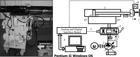
The hydraulic unit contains a pump, a valve, and a cylinder. The pump runs on a 3700 W electric motor and is capable of providing a constant supply pressure of approximately 7000 kPa at 18 liter/minute. The electro-hydraulic valve is a low bandwidth, low-cost, closed-center, four-way proportional valve (Danfuss PVG-32, from Flo Draulic Inc, Canada). The positioning of the valve spool is based on the pulse width modulation principle, i.e., the desired voltage signal sent by a computer in terms of duty cycle with the full duty cycle representing the maximum voltage. The valve operates within a range of ±1.8 volt. The deadband is approximately ±0.3 volt ∼ ±0.5 volt within which the actuator resists motion. The reaction time of the valve from the neutral position to maximum spool travel is measured at around 120 milliseconds. The valve flow gain at a 20 bar pressure differential is about 10 liter/minute per unit input signal (volt). The actuator's cylinder, having an annulus area of 1140 mm², is fixed on a frame and the force is applied to the end of the piston rod (with an area of 630 mm²) of the actuator.

The contact environment is generated using a group of springs with varying stiffness. A spring is connected to the end of the piston rod while the actuator moves forth and back. The variation of stiffness of springs helps the actuator realize different environments and adjusts the parameters in the force control algorithm to adapt to them. A force/torque sensor is inserted between the environment and the end of the piston rod of the hydraulic actuator. It reads the contact force with the accuracy of 1% and sends a measured signal to the PC computer.

The PC computer, equipped with a DAS-1601 data acquisition board from Keithley Instruments Inc, USA, plays a central role in controlling the hydraulic actuator. The A/D conversion unit of the data acquisition board is 12-bit, which is used to transfer the measured force signal in voltage into a digital signal. The feedback signal is used to generate the desired pulse-width-modulation control signal which will be the input to the hydraulic valve amplifier circuit. The step response experiment of the test station shows that, given an environmental stiffness of 40 kN/m, the time constant, T, is approximately 0.1 second. Based on the theory of sampling (Iserman 1981), the maximum sampling interval can be chosen as 0.05 second. The sampling time, in the experiments of this study, was chosen between 0.02 second.

Mathematical Model

The test station displayed in Figure 1 works in constant pump pressure mode with a closed-center valve. The input signal controls the fluid flow rates to change the line pressures. The resulting hydraulic force produces a piston displacement, y. Consider Coulomb friction, viscous friction, and the net force, f _a  = P _i A _i  − P _o A _o , the piston's dynamics is:

where P _i and P _o are the line pressures at two sides of the piston rod, A _i and A _o are the corresponding piston areas, m is the piston mass, g(..) is a nonlinear function representing Coulomb and viscous frictions. f denotes the contact force.

The derivatives of the line pressures are controlled by the following equation:

where β is the fluid bulk modulus; H _l and L _l are the high and low limits of the piston displacement, respectively; V _i and V _o are the volumes of fluid in the connecting lines, respectively.

The input signal, u, controls the spool displacement, x _sp , to generate necessary flow rates Q _i and Q _o (Merritt 1967):

where P _s and P _r are the supply and return pressures, respectively; c _d is the orifice coefficient of discharge; ρ is the mass density of the fluid; and Δ_o(..) describes the nonlinear relationship between the orifice area and the displacement of the spool valve.

By combining the aforementioned two equations and considering that the contact force is a function of the position displacement of the piston rod, we can have the following nonlinear autoregressive moving average (NARMA) model:

where Γ(..) represents the nonlinear relationship between the previous inputs and contact forces and the one-step ahead contact force output.

OUTLINE OF THE CONTROLLER

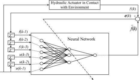
Neural Networks Modeling and Training

A multilayer feedforward neural network (NN) with one hidden layer is chosen to model the hydraulic force system, Γ(..). With reference to Figure 2, the NN can be described as:

FIGURE 2 Training a multilayer neural network using NARMA model.

where p (t) = [f(t − 1)f(t ⁻2)f(t − 3)u(t − 1)u(t − 2)u(t − 3)]T and (t) is a function of six inputs and one output, respectively;

and b ² are weight matrices and bias vectors in the hidden layer and output layer; is tan-sigmoid type activation function vector in the hidden layer (s₁ is the number of nodes in the hidden layer).

The Levenberg–Marquardt back-propagation learning algorithm was used to train the network, i.e., given a performance index, , where , with Newton's method, the modification of an n-dimensional variable vector x , in the descent direction, is

where

and J is the Jacobian matrix.

Since the term,

is difficult to calculate for most application cases, in the Levenberg–Marquardt algorithm, an adaptive factor μ is used to represent it:

In Equation (7), I is an identity matrix and μ is adaptively adjusted to make the algorithm converge faster. The parameter, μ, is increased whenever a step results in a smaller value of E _N ( x ). Otherwise, μ is decreased. Notice that when μ is large, the algorithm becomes the steepest gradient descent, while for a small value of μ, the algorithm becomes Gauss–Newton. The Levenberg–Marquardt algorithm is called as a trust region modification to Gauss–Newton. The Levenberg–Marquardt back-propagation algorithm is described in details elsewhere (Hagan and Manhaj 1994). The method, although very effective, is computationally intensive. A modification to this method has been proposed (He, Sepehri, and Unbehauen 2001), which allows updating the weights and biases layer-by-layer (starting from the output layer). In this way, only the Jacobian matrix containing the weights and bias in one layer is solved at a time. Therefore, less memory is required and convergence is faster. The modified Levenberg–Marquardt back-propagation algorithm is used in the article for training the neural network.

Predictive Control

A predictive control algorithm aims at good performance of a system a few steps ahead. Based on the prediction of future outputs from the mathematical model of a system, the predictive control algorithm normally produces a sequence of future control signals by minimizing the error between desired outputs and model outputs.

There are many predictive algorithms. Compared to other predictive algorithms, the generalized predictive control algorithm, which was introduced by Clarke, Mohtadi, and Tuffs (1987), has the following advantages: 1) robustness against unknown parameters and unknown order of the systems; 2) good adaptation of highly nonlinear systems and multivariable plants. In this article, we will use the algorithm to control the contact force of the hydraulic actuator.

Given a controlled autoregressive integrated moving average (CARIMA) model as follows:

where A(q ⁻¹) and B(q ⁻¹) are polynomials, of degree n _a and n _b , in the backward shift operator q ⁻¹ and Δ = (1 − q ⁻¹); ξ(t) is an uncorrelated random sequence; u(t) and y(t) represent the input and the output, respectively.

The objective of a predictive control algorithm is to decide a set of n-step ahead control signals based on j-step ahead predicted plant output, ŷ(t + j), so that the error between the desired outputs and the predicted plant outputs is minimal. The j-step ahead predicted plant output can be written as follows:

where E _j (q ⁻¹) and F _j (q ⁻¹) are uniquely defined polynomials of orders (j − 1) and n _a , respectively. The coefficients in E _j and F _j are computed, recursively, as follows:

with initial condition

Since the disturbance consists of only the unknown future values, the optimal predictor is

where .

Considering the prediction at nth-step ahead point, the optimal predictor is written as follows:

where ; u  = [Δu(t), Δu(t + 1),…, and

The vector, f _k , is composed of signals which are known at the time t,

From Equation (14), one can have

For g _ji in Equation (15), j presents jth-step ahead prediction and i presents the coefficient of the backward shift operator q ⁻ⁱ . Since the first j terms in G _j (q ⁻¹) are parameters of the step-response, g_ji = g_i, which is independent of the particular G_j (q ⁻¹) polynomial. The matrix G is then written as

Based on the prediction of future outputs, the GPC algorithm produces a sequence of future control signals by minimizing the following performance index:

where n ₁ is the minimum output horizon; n ₂ is the maximum output horizon; n _u is the control horizon; and λ(j) is a control weighting sequence that is usually set to a constant λ;y _d (t + j) is the j-step ahead desired output.

Minimizing the performance index produces the following control increment vector:

where and I is an identity matrix. The first element of vector, Δ u , is the current control input increment.

The parameters n ₁, n ₂, n _u , and λ in the performance index can be adjusted to produce a satisfactory response of the system. The parameter, n ₁, can be normally set to 1 with no loss of stability. The parameter, n ₂, is approximately equal to the rise time of the system. When more future control increments are taken into minimization, the system response is more stable. Notice that the GPC algorithm assumes that after n _u (< n ₂) number of time steps, the control signal is held as a constant. Finally, the control sequence, λ, acts as a damping agent for the system (Clarke et al. 1987).

Since the real control signal in the CARIMA model is u, other than Δu, we have

where λ _c is called a relax factor, which is used to adjust the amount of the input increment for a practical application.

Instantaneous Linearization of Neural Model

We have shown earlier that the hydraulic force system can be described by NARMA model (4). In order to apply the GPC algorithm to the model, the instantaneous linearization of the neural model around the current operating point (Sorensen 1994) is exploited.

Neural approximation of the hydraulic force system, described by Equation (4) can be written as follows:

The current state, x , is a vector composed of the arguments of the function N:

Linearizing the function, N, around the current state, x(t _i ), at t = t _i , to obtain the instantaneous linearized model:

where

For the neural network represented in Equation (5), the parameter vector is given by:

where

The matrices W ₁, W ₂, and b ₁ will be obtained from Equation (5) and updated by Equation (20).

Although we use the instantaneous linearization of the nonlinear model (20) at each sampling moment to provide predicted parameters to the model (9) in the GPC algorithm, the nonlinear neural model is recursively updated based on the error between the measurement and the output of the neural model. Therefore, the major difference between the proposed methodology and a normal linear model is that it retains the nonlinear characteristics of a physical system by using a nonlinear model approximation and extracts a linear model using instantaneous linearization at each sampling instant to feed the GPC algorithm, which requires the parameters from a linear model.

SIMULATION AND EXPERIMENTAL RESULTS

Pretraining of a Multilayer Feedforward Neural Network

First, the modeling and predictive capabilities of the proposed neural model are experimentally evaluated. A spring of 40 KN/m stiffness was used as the force contact environment. The amplitude-modulated, pseudo-random binary sequence (APRBS), i.e., pseudo-random binary sequence signals with the amplitude being modulated by a uniformly distributed number, was used as the input signals. Figure 3 shows the input signal (in volts) and the measured contact force output (in KNS). The sampling time for this experiment was about 0.02 second and 1497 sampling data were obtained within the time duration of 30 seconds.

FIGURE 3 Experimental input–output data for pretraining a neural network.

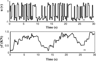
The neural network in Equation (5) was used to approximate the input and output data. The hidden nodes were chosen as three. The weights and biases were initialized with random numbers uniformly distributed over the range from − 1 to 1. After 150 epochs with the modified Levenberg–Marquard back-propagation learning algorithm, the root mean squares (RMS) of error was monotonically reduced to 0.0098 KN. The 30-step ahead prediction of the output, using the instantaneous linearized neural mode, was tested. The RMS of error for the 30-step ahead prediction was 0.074 KN, which is four times smaller than the error of 0.24 KN obtained by a normal linear model with the least mean square method.

Simulation of Neural Predictive Control

The simulation was completed using MATLAB software on a PC with Intel Pentium IV 2.4GHz CPU, manufactured by HP INC, California, USA.

The mathematical model previously described is used as the controlled actuator system. In this model, the coefficient of viscous friction and the coefficient of Coulomb friction were chosen as 1600 Ns/m and 0 Nm, respectively. The supply and return pressures are 400 psi and 0 psi, respectively. The piston mass was 20 kilograms. The fluid bulk modulus of the hydraulic system was chosen as 4e⁵ psi. The deadband of the actuator response to the input voltage was chosen as 0.3 volt. The high and low limits of the piston displacement, H _l and L _l , were 1.04 m and 0 m, respectively. The volumes of fluid in the connecting lines, V _i and V _o , were chosen as 0.015 m. The maximum spool displacement, x _spmax , is 0.002415 m. The equivalent flow coefficient was chosen as The nonlinear relationship between the orifice area and the displacement of the spool valve, Δ _o , was approximated as the variable, x _sp , to the third power with the deadband of 0.3. The fourth order Runge–Kutta method was used to solve the group of differential equations to achieve the acting force under a certain environment.

The calculated force was used to online train a multilayer feedforward neural network given by Equation (5). The initial weights of the neural network were obtained from pretraining. The modified Levenberg–Marquardt algorithm was used to online train the neural network. The length of the window was chosen as five input/output data. The error goal in root mean square error was chosen as 0.06. The adaptive factor, μ, was chosen as 0.01. The factor β was chosen as 1.2 for the increment of the adaptive factor and 0.9 for the decrement of the adaptive factor.

The trained neural model was instantaneously linearized. The parameters of the instantaneous linear model were used in the GPC algorithm to generate the desired control signal. The parameters in the GPC algorithm were chosen as n ₁ = 1;n _u  = 1;n ₂ = 30;λ = 0.1 and the relaxing factor for the increment input signal was 0.2.

The simulations were implemented to complete the following control duty: the value of a desired force was changed between 200 Newtons and 800 Newtons with a time interval of 5 seconds. The neural network was online trained to identify the variation of the environment. The input to the neural network was the measured force signal with a sampling interval of 0.02 second. Based on the parameters provided by the instantaneous linearized neural model, the GPC algorithm was used to calculate the desired input signal. The input signal was sent to the valve circuit, which was described by the first-order differential equation with a time constant of 0.02 seconds, to control the acting force in the mathematical model provided earlier.

Figure 4 provides the force response (in KNs) and the pertaining control signal (in volts) via time. From the result, we can see that the force response can track the desired force well. Since the control signal is proportional to the derivative of the force signal, when the desired force is changed, the resultant control signal will fast regulate the acting force to follow the desired force. When the control signal is within the deadband and the force output of the system will keep constant.

FIGURE 4 Desired force (– –) and force response (-) with control input u (simulation: stiffness = 40 KN/m).

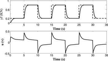
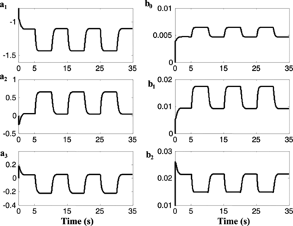
Figure 5 displays the instantaneously linearized parameter a_{j (j=1,2,3)} and b_{j (j=0,1,2)}. According to the variation of the desired force, the parameters also change periodically. The parameters a₁, a₂, and a₃ represent the influence of the forces in two previous sampling times to the current force output and the parameters b₀, b₁, and b₂ represent the influence of input signals to the current force output. Among the parameters, b₀, b₁, and b₂, the parameters b₁ and b₂ play more important roles since the average values of both parameters are around 0.025, which is much larger than the average value of parameter b₀—0.005.

FIGURE 5 Parameter estimations pertaining to Figure 4 (experiment).

In the simulation, the disturbances existing in the real system were not considered in the model. Therefore, the trajectory was tracked in an ideal environment than that in practice cases. Nevertheless, it proved that the algorithm is principally feasible and the performance of the controlled system was satisfactory.

Experimental Test of the Neural Modeland Predictive Controller

The experiments focused on the capability of neural networks to handle uncertain and nonlinear environments. To avoid a possible large overshoot that could easily overload the force sensor, the weights obtained from the pretraining of the neural network were taken as initial weights.

The experimental conditions were similar to that in the simulation, i.e., the initial condition for training the neural network and the parameters in the GPC algorithm and the desired force trajectory were the same as those in the simulation. However, the real actuator system was used here and the C code compiled by the Borland C compiler was used to generate the machine code. The measured force signal was achieved through the DAC1601 data acquisition board. The generated control signal was sent to the valve circuit via the same data acquisition board. To ensure that the piston was always in contact with the environment, the rod-end was initially positioned to apply a force around 80 N against the springs.

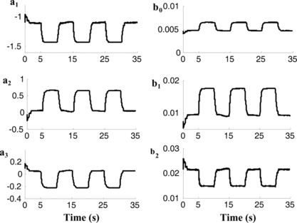
Figure 6 shows the contact force response and the pertaining control signal with the stiffness of the spring as 40 KN/m. Due to the application of a closed-loop system, the neural network takes about 1 second (50 epochs) to adapt the model and environment. After 1 second, it can be seen that the neural adaptive controller could control the system to follow the desired output closely, despite the friction and unknown deadband area. The control result reaches the desired design objective. Figure 7 shows the change of parameters of the instantaneous linearized neural model. The estimated parameters are close to the parameters obtained from simulation in spite of some noise from real measurement sensors and devices.

FIGURE 6 Desired force (– –) and force response (-) with control input u (experiment: stiffness = 40 KN/m).

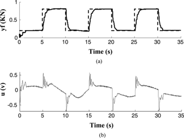
FIGURE 7 Parameter estimations pertaining to Figure 6 (experiment).

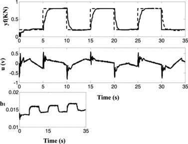
In order to test the capability of the neural adaptive force controller to adapt to different environments, the stiffness of the spring was changed to 25 KN/m. The same parameters were used in the GPC algorithm. Figure 8 shows the contact force and input signal as well as parameter b ₁. Since the spring became soft, the value of estimated b ₁ was vibrated around the desired value. However, after about a 2 second online training of the neural network to adapt to the new environment, the control result is quite comparable to the result obtained with the environment of 40 KN/m stiffness.

FIGURE 8 Desired force (– –) and force response (-) with control input u (experiment: stiffness = 25 KN/m).

CONCLUSIONS

This paper presented design, simulation and experimental evaluation of a neural-based adaptive predictive force controller for an industrial hydraulic actuator. First, it has been shown that the instantaneous linearized neural model can be used for a multistep prediction of such actuator force control systems. The parameters obtained from this model can be then applied to the GPC algorithm to control the acting force under an unknown environment. Simulation and experimental results have demonstrated that the resultant algorithm can adapt well to different environmental stiffness despite high nonlinearity and uncertainty existing in the hydraulic actuator systems.

The experiments were conducted at the Experimental Robotics and Tele-Operation Laboratory at the University of Manitoba. The author thanks Drs. Nariman Sepehri, Kamayar Ziaei, and David Niksefat for their many helpful discussions and technical supports to the research work.

REFERENCES

- Chen , J. and Y. Lu. 1994 . The variation of oil effective bulk modulus with pressure in hydraulic systems . ASME. J. Dynam. Syst. Measure., Contr . 116 : 146 – 150 .
- Clarke , D. W. , C. Mohtadi , and P. S. Tuffs. 1987 . Generalized predictive control-Part I: The basic algorithm . Automatica 23 : 137 – 148 .
- Conrad , F. and C. Jensen. 1987 . Design of hydraulic force control systems with state estimate feedback . Proc. IFAC 10th Triennial Congress , Munich , Germany , 307 – 312 .
- Daachi , B. and A. Benallegue. 2003 . A stable neural adaptive force controller for a hydraulic actuator . J. System Control Engineering 217 : 303 – 310 .
- Duchemin , D. , P. Maillet , P. Poingnet , E. Dombre , and F. Pierrot. 2005 . A hybrid position/force control approach for identification of deformation models of skin and underlying tissues . IEEE Trans. Biomedical Engineering 52 : 160 – 170 .
- Hagan , M. T. and M. B. Manhaj. 1994 . Training feedback networks with the Marquadt algorithm . IEEE Trans. Neural Networks 5 : 980 – 993 .
- He , S. , N. Sepehri , and R. Unbehauen. 2001 . Modifying weights layer-by-layer with Levenberg–Marquardt backpropagation algorithm . Int. J. Intelligent Automation Soft Computing 7 : 233 – 247 .
- Hornik , K. , M. Stinchcombe , and H. White. 1990 . Universal approximation of an unknown mapping and its derivative using multilayer feedforward networks . Neural Networks 3 : 551 – 560 .
- Iserman , R. 1981 . Digital Control Systems. New York : Springer-Verlag .
- Jaax , K. and B. Hannaford. 2004 . Mechatronic design of an actuated biomimetic length and velocity sensor . IEEE Trans. Robotics and Automation 20 : 390 – 398 .
- Kiguchi , K. and T. Fukuka. 1999 . A survey of force control of robot manipulator using soft computing techniques . IEEE SMC'99 Conference Proceedings 2 : 764 – 769 .
- Kwan , C. M. , A. Yesildirekm , and F. L. Lewis. 1999 . Robust force/motion control of constrained robots using neural network . Journal of Robotic System 16 : 697 – 714 .
- Lee , H. K. , G. S. Choi , and G. H. Choi. 2002 . A study on tracking position control of pneumatic actuators . Mechatronics 12 : 813 – 831 .
- Merritt , H. E. 1967 . Hydraulic Control Systems . New York : John Wiley and Sons .
- Parnichkun , M. and S. Kaitwanidvilai. 2005 . Force control in a pneumatic system using hyfrid adaptive neuro-fuzzy model reference control . Machatronics 15 : 23 – 41 .
- Sorensen , O. 1994 . Neural Networks in Control Applications , PhD thesis , Denmark : Aalborg University .
- Zeng , G. and A. Hemami. 1997 . An overview of robot for force control . Robotica 15 : 473 – 482 .