ENSEMBLING REGRESSION MODELS TO IMPROVE THEIR PREDICTIVITY: A CASE STUDY IN QSAR (QUANTITATIVE STRUCTURE ACTIVITY RELATIONSHIPS) WITH COMPUTATIONAL CHEMOMETRICS

Abstract

The last several years have seen an increasing emphasis on mathematical models, both based on statistics and on machine-learning. Today Bayesian nets, neural nets, support vector machines (SVM), and induction trees, are commonly used in the analysis of scientific data. Moreover, a recent emphasis in the modelling community is on improving the performance of classifiers through ensembling more different and accurate models in order to reduce the prediction error. Ensembling in fact is a way of taking advantage of good models that make errors in different parts of the data space. We will outline the developments in model construction and evaluation through those techniques justify their use and propose some quantitative structure activity relationships (QSAR) and models based on ensembling. The models presented here are in the area of predicting acute toxicity for the purpose of regulatory systems. The emphasis is on the better performances of ensembles, since the general goal of delivering usable QSAR models requires others that are out of the scope of this article.

INTRODUCTION

The development of computer programs capable of containing in explicit form the knowledge about some domain was the basis of the development of expert systems in the 1970s (Jackson 1999). Soon expert systems moved from the initial rule-based representation to the modern modelling and interpretation systems. Most of the emphasis in the beginning has been on the idea of making use of more representations of the problem, more paradigms of knowledge representation, and more algorithms to find a solution. A seminal work by Gallant (1993) introduced a way to look at both neural networks and rule-based systems. In his approach, a net built from data and absent of symbolic knowledge, is used to extract rules. This idea developed in the artificial intelligence (AI) community in the well-known area of integrating connectionist and symbolic systems.

In the same year the starting machine-learning community developed another way to make use of data in the absence of knowledge, which led to the development of inductive trees, well exemplified by C4.5 (Quinlan 1993) and there after by the commercial system CART. Integrating different representations and solutions is a direction taken in AI in the years around 1995. The term expert system in those years was practically replaced by the term intelligent system or intelligent agent. Using different representations to reach a common agreement or a problem solution led to the idea of using computational different methods on different problem representations, so to make use of their relative strengths. Examples are the hybrid neural and symbolic learning systems (d'Avila Garcez, Broda, and Gabbay 2002). Another kind of hybrid intelligent system is the neuro-fuzzy system (Funahashi 1989) that combines connectionist and symbolic features in the form of fuzzy rules.

While the neural representation offers the advantage of homogeneity, distribution, and parallelization, and of working with incomplete and noisy data, the symbolic representation brings the advantages of human interpretation and knowledge abstraction (Neagu and Gini 2003).

A fundamental stimulus to the investigations of integrated systems is the awareness that combined and integrated approaches will be necessary to solve real-world problems using AI tools. Research in this area is very active in the different traditional tracks as the integrations of neural networks with expert systems, fuzzy systems, and global optimization algorithms, to the hybridization of soft computing with other machine-learning techniques as support vector machines, rough sets, Bayesian networks, probabilistic reasoning, and statistical learning. Recently, such systems become popular due to their capabilities in handling complex problems, involving imprecision, uncertainty, and vagueness, high-dimensionality—all of them to be handled in domains as financial prediction (Chen and Wang 2004).

Independently, a similar evolution in the pattern recognition community proposed to combine classifiers. In this area, most of the intuition started with a seminal work, about bagging classifiers (Breiman 1996; Avnimelech and Intrator 1999), which opened the way to ensemble systems (Bauer and Kohavi 1999; Dietterich 2000; Freund, Yishay, and Schapire 2004). Combining the predictions of a set of classifiers has shown to be an effective way to create composite classifiers which are more accurate than any of the component classifiers (Ho, Hull, and Srihari 1994).

In literature we can find at least two main streams, namely, “ensembles'’ of highly correct classifiers that disagree as much as possible, and “mixture of expert's, built on the idea to train individual networks on a subtask, and then combine their predictions with a “gating” function that depends on the input. Basic combinations like a majority vote or an average of continuous outputs are sometimes effective. Finally, it is possible to train the output classifier separately using the outputs of the input classifiers as new features. There are many methods for combining the predictions given by component classifiers, as voting (Bauer and Kohavi 1999), combination (Kittler, Hatef, Duin, and Matas 1998; Ho 2002), ensemble (Krogh and Vedelsby 1995), and a mixture of experts (Jacob, Jordan, Nowlan, and Hinton 1991).

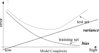
Why ensembles work and why they outperform single classifiers can be discussed considering the error in classifiers. Usually the error is expressed (Friedman 1997) as:

where the noise is irreducible while the other components are:

	bias, the expected error of the classifier due to the fact that the classifier is not perfect;
	variance, the expected error due to the particular training set used.

We observe that models with too few parameters can perform poorly, but the same applies to models with too many parameters. In fact a model that is too simple, or too inflexible, will have a large bias; a model that has too much flexibility will have high variance. Usually, the bias is a decreasing function of the complexity of the model, while variance is an increasing function of the complexity, as illustrated in Figure 1.

FIGURE 1 The error function for different complexities of the model.

The concepts of bias and variance are of help in understanding the balance between the conflicting requirements of fitting our training set accurately to obtain a good predictor. We seek a predictor that is sufficiently insensitive to the noise on the training data, to reduce variance, but which is also flexible enough to approximate our model function and so minimize bias. There is a trade-off between the two components of the error, and balancing them is an important part of error reduction. Increasing complexity of the model is not (in general) a way to reduce the error, so simple models that fit enough data are usually developed.

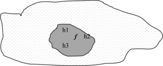
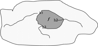
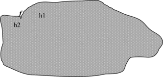
At least three reasons why ensembles are effective in reducing the error have been indicated in Dietterich (2000) and are briefly illustrated:

• Statistical Problem: There are many hypotheses with the same accuracy, and the learning algorithm chooses one of them, but an ensemble mixes them to better approximate the true hypothesis, as shown in Figure 2.

• Computational Problem: The learning algorithm cannot guarantee reaching the best hypothesis, so mixing the different hypothesis improves the result, as shown in Figure 3.

• Representational Problem: The hypothesis space does not contain any positive approximation of the target classes, so additional hypotheses near the border are combined as shown in Figure 4.

Our application domain is in chemometrics the information aspects of chemistry. Chemometrics encompasses the basic steps of data analysis, experimental design, and modelling. While the basic of chemometric strategies evolved from statistical experimental design, which gives the basis for the ways to generate a set of examples, reduce attribute dimensionality, and attribute value ranges, transform data to simplify the response function, the methods for model extraction belong to different areas such as pattern recognition, clustering, and machine-learning.

FIGURE 2 Statistical problem.

FIGURE 3 The computational problem.

FIGURE 4 The representational problem.

One of the most active areas in chemometrics is quantitative structure activity relationships (QSAR), developed in the last 40 years to assess the value of drugs, and more recently proposed as a way to assess general toxicity, as well as a way to obtain new knowledge from data. Quantitative structure activity relationships can be both regression or classification: for drug activity and toxicity to a given target, most of the QSAR models are regressions, referring to the dose giving the toxic effect in 50% of the animals. The correct modelling of QSAR derives from “postulates” as defined from evidence and theory, as so expressed:

	The molecular structure is responsible of all the activities shown.
	Similar compounds have similar biological and chemico-physical properties (Meyer 1899).
	Hansch (1963) postulate: biological system + compound gives answer = f1 (lipolificity) + f2 (electronics) + f3 (steric) + f4 (molecular property).
	Congenericity postulate: QSAR is applicable only to similar compounds.

This definition of QSAR makes it evident that the locality of the model should be preserved and generalization requires attention.

Finally, the predictive toxicology problem is the problem of developing predictive models, in order to obtain improved applicability of these systems to real regulations to acquire knowledge from data to speed up scientific discovery. The final target of this research is to work in silico, not in vivo(a “virtual” laboratory for toxicity). This trend is not new in chemistry, which is largely a computer-based area: computer models and computation are present in any area of analysis and synthesis, where models are searched to provide an explanation to the experimental results.

Ensembles are appealing in QSAR to improve the accuracy of statistical models. As widely known, no single method can be considered as the only way to predict toxicity (Benfenati, Mazzatorta, Neagu, and Gini 2002). Several methods can give good predictions in a comparable way, since each approach can incorporate some parts of knowledge. Examples of application of those concepts in chemometrics are appearing in literature (Merkwirth, Mauser, Schulz-Gasch, Roche, and Lengauery 2004). In our previous research, we have extensively combined local experts to assess good predictive models of challenging data, as the Duluth data set of environment protection agency (EPA) which contains toxicities against the fathead minnow (Koening, Gini, Craciun, and Benfenati, 2004; Gini, Craciun, Koening, and Benfenati 2004), the carcinogenicity set from RTECS and the gold data set (Gini, Lorenzini, Benfenati, Brambilla, and Malve 2001).

In the following sections we will develop our approach creating models and ensembling them. In the present investigation, we approach the area of QSAR for regulatory purposes; we work on the dataset of pesticide as developed in the EU project Demetra to develop basic models on different animal endpoints and to integrate them to get a final model for public release (Benfenati 2007). We report here on some of this development.

THE QSAR PROBLEM IN THE ENSEMBLING PARADIGM

Different computer-based approaches to analyze chemical and biological information and to automatically discover knowledge implicitly contained in the data have been reported (Gini and Katrizky 1999).

To get an ensemble we need to build basic models that are accurate and diverse. We start building basic models in various techniques, so to guarantee that they are independent, we check their results and finally investigate ensembles. The models produce an equation or a subsymbolic representation of the correlation between the structural descriptors of the molecules and the biological property considered. Usually we apply a logarithmic transformation of the output to reduce its range.

The chosen method for ensembling is stacking classifiers through a learning system able to integrate them. While inputs to the basic models are the chemical descriptors, input to the ensemble model are the n values predicted for each molecule by the n integrated models; the output is always the toxicity for that molecule. The models can be chosen and compared using a graphical method, as we show in the subsequent section.

In many cases, published QSAR models implement a leave-one-out cross-validation procedure and compute the cross-validated R ², called q ². A high value of q ² (for instance, q ² > 0.5) is considered an indicator or even the ultimate proof that the model is highly predictive. A high q ² is the necessary condition for a model to have a high predictive power; however, it is not a sufficient condition. Besides the wide accepted criteria of checking q ², some additional more strict conditions should be imposed, as we will list.

Besides the better prediction value we can obtain from the combined model, we may want to understand its statistical meaning in a more complete way. This idea is at the basis of the receiver operating characteristic (ROC) curves for classifiers, and has been exemplified in the recent predictive toxicology challenge (Helma and Kramer 2003). The ROC curves have proven to be a valuable way to evaluate the quality of binary classifiers. The expected performance of a classifier can be characterized by the area under the ROC curve (AUC), which gives a simple way to individuate a valid classifier that should have an AUC > 0.5.

The authors of Bi and Bennett (2003) devised a methodology for regression problems with similar benefits to those of ROC curves. In regression, existing measures of residuals such as mean-squared error, mean absolute deviation, R ², and q ², provide only a single snapshot of the performance of the regression model; the regression error characteristic (REC) curves instead plot the error tolerance on the x-axis versus the percentage of points predicted within the tolerance on the y-axis (accuracy).

The resulting curve estimates the cumulative distribution function of the error, which can be defined as the difference between the predicted value f(x) and the actual value y of response for any point (x, y), or the squared residual (y − f(x))². Accuracy is defined as the percentage of points that are fit within the tolerance. If we have zero tolerance, only those points that the function fits exactly would be considered accurate. If we choose a tolerance that exceeds the maximum error observed for the model on all of the data, then all points would be considered accurate. So as the tolerance increases, the accuracy also increases and eventually goes to 1. The area over the REC curve (AOC) is a measure of the expected error for a regression model (Bi and Bennett 2003), since it is an approximation of (1 − R ²).

The range of the tolerance adjusts the appearance of REC curves. We scale the box to draw the REC curves for our ensembles using the average model, i.e., a model with all points equal to the mean of the response of the basic models on the training data. The x-axis starts with 0 and ends at the largest value of the errors obtained by the average model. It is easy to see the best model checking the dominant curve or the curve that first reaches accuracy 1.

All the REC computation in the following are done using Matlab functions.

Besides REC, we applied the additional conditions, proposed by Golbraikh and Tropsha (2002), to conclude if a QSAR model has an acceptable prediction power. We check that both the q ² in cross-validation and the R ² on an external test set are above a minimum value, and that the regression line has a correct slope and intercept, as expressed in the following conditions:

To compute the conditions in Equation (2), we proceed as in Equation (3). If , and y _i are the predicted and actual logProperty values, and respectively, are the average value of the predicted and observed logProperty. The parameters are calculated as follows:

BUILDING AND INTEGRATING MODELS

In the European Union pesticides are currently assessed via the EU Directive 91/414/EEC (EEC, 1991). This directive and the associated annexes cover the risk to the operator, consumer, and environment. Annex II outlines what data are required on the active substance. The risk to the environment covers both the fate and behavior of an active substance (i.e., exposure) as well as its possible effects to nontarget organisms. Nontarget organisms considered under 91/414/EEC include: birds, mammals, aquatic life (fish, aquatic invertebrates, algae, and aquatic plants), non target arthropods, honeybees, earthworms, soil macro-invertebrates, soil microbial processes, and terrestrial nontarget plants.

Table 1 provides part of the toxicity studies that may be requested when an active substance is considered under 91/414/EEC.

TABLE 1 Ecotoxicological Data Required Under 91/414/EEC (Partial List)

Annex Point	Data Requirement	What Is Required?
8.1	Effects on Birds
8.1.1	Acute oral toxicity	One study is required either mallard duck, Japanese quail, or bobwhite quail.
8.1.2	Short-term dietary toxicity	One study is required either the bobwhite quail or the mallard duck.
8.1.3	Subchronic toxicity and reproduction	Test species are usually either the bobwhite quail, Japanese quail, or the mallard duck.
8.2	Effects on Aquatic Life
8.2.1	Acute toxicity to fish	A warm and coldwater fish species must be tested. These are usually the bluegill sunfish and the rainbow trout.
8.2.2	Chronic toxicity to fish	Generally a study conducted to OECD 204/215 guideline.
8.2.2.1	Chronic toxicity test on juvenile fish	Generally a study conducted to OECD 204/215 guideline.
8.2.2.2	Fish early life stage toxicity test	Test species are usually fathead minnow or rainbow trout.
8.2.2.3	Fish life cycle test	Generally a study submitted to US EPA protocol 72-5 is submitted.
8.2.3	Bioconcentration in fish	Generally a study conducted to OECD 305 guideline.
8.2.4	Acute toxicity to aquatic invertebrates	Generally a study conducted to OECD 202 guideline.
8.2.5	Chronic toxicity to aquatic invertebrates	Generally a study conducted to OECD 211 guideline.
8.2.6	Effects on algal growth	Generally a study is conducted to OECD 201 guideline.
8.2.7	Effects on sediment dwelling organisms	Usually a study conducted along the lines of the draft OECD.
8.2.8	Aquatic plants	Usually a study conducted along the lines of the draft OECD guideline 221.
8.3	Effect on Arthropods
8.3.1	Bees
8.3.1.1	Acute toxicity	Study covers the contact and oral toxicity of the active substance.
8.3.1.2	Bee brood feeding test	Studies conducted according to Oomen et al. (1992).
8.3.2	Other arthropods	Data may be submitted on two standard sensitive species as well as two crop relevant species.

From Table 1 we can observe that important endpoints are avian acute toxicity, avian dietary toxicity, and acute toxicity on bees.

In previous studies on the classification of toxicity of pesticides, several models have been proposed. For instance, classifiers were combined, which improved the overall results (Benfenati et al. 2002) on rat toxicity for 57 organophosphorus pesticides. Good results were obtained, but there is a need to create models on different chemicals since modern pesticides are based on very different chemical structures, which usually means different mechanisms of action. There has been an interest in understanding and explaining some specific activities, for instance, of compounds with anti-cholinesterase activity (Lin, Lai, and Liao 1999), but in general we do not have knowledge of the existence of a specific receptor with a given structure for each of the pesticides. So our models have to take chemicals of different classes and correlate the chemical structure to the effect.

In the basic QSAR approach, given the compound structure there are different ways to compute descriptors that account for the geometry, physics, and activity of the molecule. We had several choices, such as physico-chemical, namely, log P, steric parameters, electronic parameters, or topological indices. A large number, about 3000, can be easily computed from available software. We used only 2D descriptors, namely, descriptors that are computed from the 2D structure and do not require the optimization the molecular structure in 3D space.

After the preparation of the data sets, as illustrated in (Benfenati (2007), and the computation of descriptors, a group of partners developed the first level models using various methods. After choosing reasonably accurate models, we integrate them.

We take, as the basic measure of the value of our ensemble, the model obtained averaging the single component models. The average model is always an improvement of the basic models since it reduces the variance of the error (Bauer and Kohavi 1999). Using the stacking approach other kinds of hybrid models are then built and checked against the average model, and retained only if they are doing better.

Developing the First Level Models

We illustrate here an experiment on the Oral Quail LD50 endpoint, studied in the above-mentioned Demetra project. The data set contains heterogeneous chemicals and is available on the Demetra website¹ and also given in the Appendix A. We used various machine learning algorithms and checked their prediction both in leave-more-out and over an external test set.

APPENDIX A Molecules and Toxicity for Oral Quail. The Elements in Grey Have Been Left Out During Training to be Used as a Test Set for the Ensemble Model

ID	Chemical	TOXICITY (Log(Kg/mmol))
3	DCDMH(Glychlor Formulation)	−0,9397318
4	Dichloropropene	−0,136638
21	Alachlor	−0,7447597
22	Aldicarb	1,9784088
25	Ametryn	−0,9954303
26	Amitraz	−0,4289921
29	Atrazine	−0,6392374
30	Bendiocarb	1,0700379
32	Bensulide	−0,5423496
35	Bromacil	−0,9606828
46	Carbofuran	1,6425116
48	Oxythioquinox	0,0775533
50	Chlorethoxyfos	1,0791942
51	Chlorhexidine diacetate	−0,5075817
54	Chlorophacinone	−0,1207709
58	Chlorpyrifos	1,0396619
62	Clodinafop-propargyl	−0,6190929
63	Clomazone	−1,0199695
68	Cyhexatin (Plictran)	0,1085988
75	DBNPA	−0,1654213
83	Dichlobenil	−0,598867
84	Dichlorprop(2,4-DP)	−0,1778061
85	Dichlorvos	1,3998703
87	Dicloran (DCNA)	−0,6382302
90	Dienochlor	−0,1718614
95	Dimethenamid	−0,5879298
103	Dodine	−0,3803019
104	Dowicil	−0,758412
111	Ethion	0,4783994
125	Fenridazone-sodium	−1,1728725
126	Fenthion	1,5933485
139	Formetanate Hydrochloride	0,7931
146	Hydramethylnon	−0,5677835
150	Iprodione	−0,449719
152	Isofenphos	1,5988534
157	Lithium perfluorooctane sulfonate	1,0809527
160	MCPP Acid	−0,5176683
165	Methomyl	0,8263426
176	N,N-Diethyl-meta-toluamide(DEET)	−0,8565877
185	Imidacloprid	0,2250138
187	Octhilinone	−0,2551775
188	Oryzalin	−0,1651605
194	Paradichlorobenzene	−1,0389687
195	Paranitrophenol	−0,6177862
197	Methyl Parathion	1,5418136
198	Pentachlorophenol	−0,3718638
204	Phorate	1,5705763
216	Propachlor	0,3812587
217	Propanil	0,0354397
236	Phostebupirim	1,1955043
238	Temephos	1,2311104
240	Terbufos	1,0037497
244	Thiazopyr	−0,6835594
252	Tribuphos	0,3187404
257	Triclosan	−0,4547454
262	Trimethacarb	−0,0904125
264	Uniconazole	−0,69955
273	3,5Dimethyl-1-(hydroxymethyl)pyrazole	−0,7792513
275	2,4-D Isopropyl Ester	−0,8537564
277	3-Iodo-2-propynyl butylcarbamate	−0,4256055
278	4,5-Dichloro-1,2-dithio-3-one	−0,1206928
282	Bentazon Sodium Salt	−0,6498248
285	Bifenazate	−0,5359942
297	DDAC	0,2223448
304	Dipropyl isocinchomeronate	−0,730124
307	Etridiazole	−0,3545426
311	Fluazinam	−0,583352
323	Naphthalene	−1,321932
328	Parachlorometacresol	−1,0334317
331	Pirimiphos-methyl	0,8827806
333	Prallethrin	−0,5908136
340	Thiodicarb	−0,7563429
346	Sodium dichloro-s-triazinetrione	−0,9046667
347	2-(Hydroxymethylamino)ethanol	−1,281636
351	Azinphos-methyl	0,9830382
353	Bromethalin	2,0991249
354	Bromo-3-chloro-5,5-dimethylhydantoin(BCDMH)	−0,6465026
355	Bromoxynil heptanoate	0,0349668
361	Coumaphos	2,1867433
364	Cyproconazole	0,2890089
366	Diazinon	1,767427
368	Dicamba (Acid)	0,0100171
369	Diclofop-methyl	−1,1104437
371	Endosulfan	0,9862597
372	Endothall	−0,4237939
376	Fenamiphos	2,2778956
377	Fenitrothion	1,0699752
378	Fluchloralin	−1,2939775
385	Hexazinone	−0,950355
386	Hymexazol	−1,1738945
391	Methiocarb	1,0605822
394	Methyl Bromide	0,1141264
395	N6-Benzuladenine	−0,8511258
400	Propiconazole	−0,916675
411	Sulfluramid	0,04623
412	TCMTB	−0,4428331
423	4-Aminopyridine	0,7976368
424	Chlorobenzilate	−0,2710382
425	Chloroprop, Sodium salt	−0,7717249
426	Cyromazine	−1,0309549
427	Decyl isonomyl dimethyl ammonium chloride	1,0101627
428	Dimethoxane	−0,9589313
429	Dinoseb acid (Cancelled in U.S.)	0,7785853
431	Disulfoton	1,359282
432	Esfenvalerate	0,0422519
433	Grotan	−0,8407455
434	MCPA Acid	−0,2739455
435	Mecoprop-P	−0,4054415
436	Mefenoxam	−0,5454892
437	Methamidophos	1,1453595
438	Pyrithiobac-sodium	−0,6613467
439	Sodium dodecylbenzenesulfonate	−0,5900943
440	Sulprofos	0,8364184
441	Trichlorfon	1,060428
442	Trichloro-s-triazinetrione	−0,8575006

Oral Quail Toxicity

In the Oral Quail data set, 2D descriptors were used to build the models, after considerations reported in previous QSAR analyses (Benfenati 2007). The total number of chemicals for which the LD50 is available through the Demetra project is 116. The output considered is TOXICITY (Log(Kg/mmol), reported in Appendix B.

APPENDIX B Names of the Descriptors Computed Through Dragon for the Oral Quail Basic Models

DRA0173 C-005

DRA0200 C-032

DRA0228 O-060

DRA0347 TIE

DRA0367 X1Av

DRA0405 IDDE

DRA0418 TIC0

DRA0540 T (S..S)

DRA0584 BEHm3

DRA0661 JGI6

DRA0716 MATS2e

DRA0747 GATS1e

For building the level 1 models, we used the WEKA data mining workbench created by the Department of Computer Science at the University of Waikato, New Zealand.² It comprises a wide range of different data mining algorithms for regression, classification, and clustering as well as tools for preprocessing evaluation and visualization of the data and the results. Windows XP was the operating system platform used and the Microsoft office tools were used for the data handling and preparing the data for “arff” format which is needed for WEKA. Small visual basic scripts were introduced in Excel sheets to get the desired format.

To be comparable with other models developed by other partners in the project, we chose 12 Dragon descriptors, selected after PCA analysis, namely: DRA0173, DRA0200, DRA0228, DRA0347, DRA0367, DRA0405, DRA0418, DRA0540, DRA0584, DRA0661, DRA0716, DRA0747, computed through e-Dragon.³ The external test set has been selected as 19 molecules in the space covered by the training set.

We used the criteria illustrated above for evaluating and accepting the models. In practice:

1. The value of R ² in 10-fold cross-validation (the more robust method used in WEKA instead of leave-one-out) should be greater than 0.55.

2. For choosing between the models with similar values of R ², we also kept in mind that the models should not predict a high toxic compound as a lower one, so we preferred models with less underestimated toxicity.

Some of the best models obtained are illustrated in the following. We want to observe here that many models have similar performances on the same data, so the decision of preference is not easy.

We report in Tables 2 and 3 examples of the best WEKA models obtained.

TABLE 2 NN Multilayer Perceptron Model for Oral Quail

Summary: NN, sigmoidal transfer function,six nodes in the hidden layer	10-fold cv
R ^2	0.57
Correlation coefficient	0.75
Mean absolute error	0.53
Root mean-squared error	0.68
Relative absolute error	68.23%
Root relative squared error	74.44%

TABLE 3 Pace Regression Model for Oral Quail

Summary: pace classifier regression withempirical Bayes estimator for normal mixture	10-fold cv
R ^2	0.57
Correlation coefficient	0.75
Mean absolute error	0.48
Root mean-squared error	0.59
Relative absolute error	62.61%
Root relative squared error	65.41%

The results that we have obtained are not completely satisfactory, particularly considering that errors are equally distributed and some high toxic compounds are predicted as less toxic. Therefore we investigated how to improve them through ensembling techniques.

Ensemble Models

Here we develop the combination of basic models and discuss the results obtained starting from the Oral Quail; we continue then on other endpoints as the dietary Quail and the Bee endpoints.

We start from a set of models all built on the same training set. We compute the mean model by averaging, and then we produce the ensemble model through stacking and compare their REC diagrams. We make the test on an external test set that has never been used by the classifiers.

Oral Quail

In addition to our own models, we selected four out of the many basic models developed in the Demetra (Benfenati 2007) project; we show in Table 4 their accuracy comparing their q ² and R ² values. Three of the models have very good performance and are based on different descriptors and methods as multilinear regression, Partial Least Squares (PLS), and neural nets. The first is poor but is inserted since it uses Neural Networks (NN).

TABLE 4 Basic Oral Quail Models Considered for Ensembling

	R ^2	q ^2
CSL05	0.423	0.421
CSL06	0.667	0.666
NEGRI01	0.606	0.606
NEGRI02	0.692	0.692

If we average the values computed by all the models on the training set, we get the mean model, which can be considered the first ensemble model, and whose values are R ² (mean) = 0.69; q ² (mean) = 0.67. As we see, the variance has been reduced about 20% only by averaging the models.

To improve this mean model, we must try more complex integrations, as we can see in the following.

We try a stacking method with NN with backpropagation. We define a three layer architecture with four neurons in the input layer (the four models), four neurons in the hidden layer, and one layer in the output (the toxicity). We train the net with the function “traingdx”; the activation functions are”tansig” and “lin” for the output. The results for this model are summarized in Table 5, both on the train sets and the test sets, and show an improvement over the mean model.

TABLE 5 Results for Ensemble 1 Oral Quail

			k
0.818	0.818	0.590	1.16	0.975	0.7

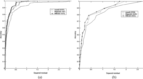
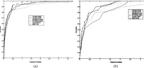
We can better analyze the models in the REC curve. we immediately see that the NN model dominates the other models (Figures 5a and 5b). We also observe that the AOC of the ensemble is minimum but the ensemble model reaches accuracy 1 after the single model Negri02. In the boxes of the REC curves, we give the value of AOC which should be minimized since it is an approximation of (1 − q ²).

FIGURE 5 REC curves for the Oral Quail on the (a) training set and (b) test set, respectively. We observe that the mean model has a nonconvex behavior and does not reach the accuracy.

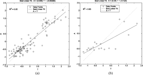
There is still a way to improve this ensemble model. We develop a new model using the training function “trainbr”, which applies Bayesian regularization, and a net with three neurons in the hidden layer, whose results are shown in Table 6. We see the regression line on the training set and the test set in Figure 6.

TABLE 6 Results for Ensemble 2 Oral Quail

			k
0.855	0.854	0.624	1.12	0.987	0.74

FIGURE 6 Regression lines for the second NN model for Oral Quail on the (a) training set and the (b) test set.

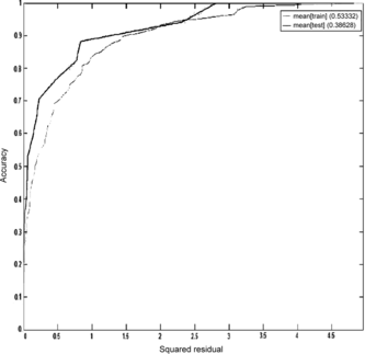
If we want to compare the two NN models, we can draw together their REC curves on the training set and the test set, as we see in Figure 7. Here we see that the second model is better that the first: it reaches unitary accuracy before and dominates the other model.

FIGURE 7 Comparison of the two NN models for Oral Quail on the (a) training set and (b) the test set.

Other Ensembling Models

Similar work has been carried out on other models. We report here about bee since it presents a new problem in model quality assessment.

For the bee endpoint, we started with the basic models of Table 7. Some of them are developed using genetic algorithms and clustering techniques. Other use the partial least squares (PLS) regression technique (projection to latent structures by means of PLS) implemented in a Simca – P8.0 package (Umetrics AB, Umea, Sweden).

TABLE 7 BASIC Models for Bee

	R ^2	q ^2
CSL01	0.607	0.606
CSL02	0.710	0.709
NEGRI04	0.658	0.658
NEGRI06	0.628	0.628

The parameters on those models are already acceptable according to the previously mentioned criteria. If we build the average ensemble model from them, we get:

The regression analysis on the mean model indicates that the slope of the regression line is much better in the test set than in the training set. We can observe this behavior also through the REC curves in Figure 8.

FIGURE 8 REC curves for the training set and test set of the mean model for bee.

We see that the accuracy on the training set is lower than on the test set. This analysis indicates that the ensemble model has a dubious value. In this case, we should go back to the first level models and check this anomaly. The real problem is that the model seems to underfit the training data, and can be a result of the scarce data available.

CONCLUSIONS

We have proposed and motivated the use of ensembling in QSAR as a way to reduce the error of the classifier. In particular, we have chosen the approach of stacking multiple classifiers to improve the performance of basic classifiers. The condition to make this ensembling useful is that basic classifiers are diverse and accurate enough. In our example, the basic classifiers chosen have been developed on the same data set by different partners and using methods going from PLS to neural networks to SVM. The full details on those models are not reported here since our discussion is about the statistical properties of the ensembles.

We have presented a step-by-step process to develop ensembles in a case of QSAR for heterogeneous compounds. We should mention that this case study is derived from the need of industry to explore QSAR methods for pesticides, considering that pesticides are of many different chemical classes, and that toxicity data are available more for old pesticides than for new ones. Since the considered compounds are really heterogeneous, we can expect that the performance of a single model is weak. We have observed that the ensemble model obtained through averaging performs better and can also make a good use of overfitted models. We need more adaptable techniques however, to integrate the models as in the developed gating network method experimented. Some of those ideas have been inserted into available methods to model pesticides, as reported in Benfenati (2007).

This exploratory study concluded that it is possible to significantly improve the performance of the QSAR model using techniques derived from machine-learning and data mining. In this study, we limited our integration to the use of a few models of good quality; the reason is that people can be more confident in the component parts. Theoretically, however, we can expect to get better performances from ensembling more many diverse models, for instance to explore a way to make use of the randomization of the feature selection method so to build models with different features instead of trying a priori to minimize their number. The cost of this ensembling, however, will be that the number of descriptors to be used will become significant.

The next step will be both the revision of the basic models as well as the exploration of ensemble an a with greater with number of basic classifiers. We feel that the statistic results will be much more significant, but that the confidence of users in the final model will be poor, since it would be impossible to say exactly what any single model is bringing into the ensemble.

We kindly acknowledge the EU projects ION for providing financial support, and Demetra for supporting Tushar Garg during his stage in Milan. Special thanks to the group of Istituto Mario Negri, Milano, and to BCX (France) for the preparation of data set.

Notes

The test set is composed of compounds with the following IDs: 32, 46, 48, 54, 75, 176, 194, 216, 277, 282, 347, 361, 385, 391, 423, 425, 431, 434, 439.

Subdivision of the data in training and test data is based on toxicity values only, and was done this way to obtain similar distributed data sets:

1. Sort toxicity values y = − Log(Toxicity [mmol/kg]).

2. 1 of 6 compounds of the sorted toxicity list is selected for the test set.

www.demetra-tox.net

www.cs.waikato.ac.nz/ml/weka

www.vcclab.org

REFERENCES

- Avnimelech , R. and N. Intrator . 1999 . Boosted mixture of experts: An ensemble learning scheme . Neural Computation 11 : 483 – 497 .
- Bauer , E. and R. Kohavi . 1999 . An empirical comparison of voting classification algorithms: Bagging, boosting, and variants . Machine Learning 36 ( 1–2 ): 105 – 139 .
- Benfenati , E. Ed. 2007 . Quantitative Structure-Activity Relationships (QSAR) for Pesticides Regulatory Purposes . Philadelphia : Elsevier .
- Benfenati , E. , J. R. Chretien , G. Gini , N. Piclin , M. Pintore , and A. Roncaglioni . 2007 . Validation of the models . In Quantitative Structure-Activity Relationship (QSAR) for Pesticide Regulatory Purposes , pp. 187 – 189 , Amsterdam : Elsevier .
- Benfenati , E. , P. Mazzatorta , D. Neagu , and G. Gini . 2002 . Combining classifiers of pesticides toxicity through a neuro-fuzzy approach . In Multiple Classifier Systems, Lecture Notes in Computer Science 2364 , Springer , 293 – 303 .
- Bi , J. and K. P. Bennett . 2003 . Regression error characteristic curves. Procs. 20th International Conference on Machine Learning (ICML-2003), Washington, DC. .
- Breiman , L. 1996 . Bagging predictors . Machine Learning 24 ( 2 ): 123 – 140 .
- Chen , S. H. and P. P. Wang . eds. 2004 . Computational Intelligence in Economics and Finance . Berlin : Springer-Verlag .
- d'Avila Garcez , A. S. , K. Broda , and D. M. Gabbay . 2002 . Neural-symbolic learning systems: Foundations and applications. Perspectives in Neural Computing . Berlin : Springer-Verlag .
- Dietterich , T. 2000 . Ensemble methods in machine learning . In Multiple Classifier Systems—1st Int. Workshop, MCS 2000, 1857, Lecture Notes in Computer Science , eds. J. Kittler , and F. Roli , Cagliari , Italy , pp. 1 – 15 .
- Freund , Y. , M. Yishay , and R. E. Schapire . 2004 . Generalization bounds for averaged classifiers . Annals of Statistics 32 : 1698 – 1722 .
- Friedman , J. 1997 . On bias, variance, 0/1 loss and the curse of dimensionality . Data Mining Knowledge Discovery 1 : 55 – 77 .
- Funahashi , K. 1989. On the approximate realization of continuous mappings by neural networks. Neural Networks 2:183–192.
- Gallant , S. I. 1993 . Neural Network Learning and Expert Systems . Cambridge , MA : MIT Press .
- Gini , G. and A. Katrizky (eds.) 1999 . Predictive toxicology of chemicals: Experiences and impact of AI tools. AAAI Spring Symposium on Predictive Toxicology SS-99-01 . Menlo Park , CA : American Association for Artificial Intelligence Press .
- Gini , G. , M. Craciun , C. Koening , and E. Benfenati . 2004 . Combining unsupervised and supervised artificial neural networks to predict aquatic toxicity . J. Chemical Information and Computer Sciences (The American Chemical Society) 44(6):1897–1902. .
- Gini , G. , M. Lorenzini , E. Benfenati , R. Brambilla , and L. Malvé . 2001 . Mixing a symbolic and a subsymbolic expert to improve carcinogenicity prediction of aromaticcompounds. Lecture Notes in Computer Science LNCS 2096 , Berlin : Springer-Verlag .
- Golbraikh , A. and A. Tropsha . 2002 . Beware of q2! J. Mol. Graph Model 20 : 269 – 276 .
- Hansch , C. , P. P. Malony , T. Fujita , and R. M. Muir . 1962 . Correlation of biological activity of phenoxyacetic acids with Hammett substituent constants with partition coefficents . Nature , 194 : 178 – 180 .
- Helma , C. and S. Kramer . 2003 . A survey of the Predictive Toxicology Challenge 2000–2001 . Bioinformatics 19 ( 10 ): 1179 – 1182 .
- Ho , T. K. 2002 . multiple classifier combination: Lessons and next steps . In Hybrid Methods in Pattern Recognition , eds. A. Kandel , and H. Bunke . World Scientific 2002. .
- Ho , T. K. , J. J. Hull , and S. N. Srihari . 1994 . Decision combination in multiple classifier systems . IEEE Transactions on Pattern Analysis and Machine Intelligence 16 ( 1 ): 66 – 75 .
- Jackson , P. 1999 . Introduction to Expert Systems, 3rd ed. Harlow, UK: Addison Wesley Longman. .
- Jacob , R. A. , M. I. Jordan , S. J. Nowlan , and G. E. Hinton . 1991 . Adaptive mixtures of local experts . Neural Computation 3 : 79 – 87 .
- Kittler , J. M. , R. Hatef , R. Duin , and J. Matas . 1998 . On combining classifiers . IEEE Trans. Pattern Analysis and Machine Intelligence 20 ( 3 ): 226 – 239 .
- Koening , C. , G. Gini , M. Craciun , and E. Benfenati . 2004 . Multi-class classifier from a combination of local experts: Toward distributed computation for real-problem classifiers . Int. J. Pattern Recognition and Artificial Intelligence 18 ( 5 ): 801 – 817 .
- Krogh , A. and J. Vedelsby . 1995 . Neural network ensembles, cross validation and active learning . In Advances in Neural Information Processing Systems , eds. G. Tesauro , D. S. Touretzky , and T. K. Leen , Cambridge , MA : MIT Press .
- Merkwirth , C. , H. Mauser , T. Schulz-Gasch , O. Roche , and T. Lengauerý . 2004 . Ensemble methods for classification in cheminformatics . J. Chem. Inf. Comput. Sci. 44 : 1971 – 1978 .
- Meyer , H. 1899 . Naunyn Schmiedebergs . Arch. Exp. Path. Pharm. 42 : 109 – 118 .
- Neagu , C. -D. and G. Gini . 2003 . Neuro-fuzzy knowledge integration applied to toxicity prediction . In: Innovations in Knowledge Engineering , eds. R. Jain , A. Abraham , C. Faucher , and B. Jan van der Zwaag , Advanced Knowledge International Pty Ltd, Ad, Australia. .
- Quinlan , J. R. 1993 . C4.5: Programs for Machine Learning . Los Altos , CA , USA : Morgan Kauffman .
- Toivonen , H. , A. Srinivasan , R. D. King , S. Kramer , and C. Helma . 2003 . Statistical evaluation of the predictive toxicology challenge 2000–2001 . Bioinformatics 19 ( 10 ): 1183 – 1193 .