APPLICATIONS OF DATA MINING TECHNIQUES TO AUTOMATIC FROG IDENTIFICATION

Abstract

An intelligent frog call identifier is developed in this work to provide the public with easy online consultation. The raw frog call samples are first filtered by noise removal, high frequency compensation, and discrete wavelet transform techniques in that order. An adaptive end-point detection segmentation algorithm is proposed to effectively separate the individual syllables from the noise. Eight features, including spectral centroid, signal bandwidth, spectral roll-off, threshold-crossing rate, delta spectrum magnitude, spectral flatness, average energy, and mel-frequency cepstral coefficients are extracted and serve as the input parameters of the classifier. Three well-known classifiers, the kth nearest neighboring, a backpropagation neural network, and a naive Bayes classifier, are employed in this work for comparison. A series of experiments were conducted to measure the outcome performance of the proposed work. Experimental results show that the recognition rate of the k-nearest neighbor classifier with the parameters of mel-frequency cepstral coefficients can achieve up to 93.81%. The effectiveness of the proposed frog call identifier is thus verified.

INTRODUCTION

Pattern recognition forms a fundamental solution to different problems in real-world applications (Kogan and Margoliash, 1998). The function of pattern recognition is to categorize an unknown pattern into a distinct class based on a suitable similarity measure. Thus similar patterns are assigned to the same classes while dissimilar patterns are classified into different classes.

In speech recognition, a source model is assumed and the signal is expected to obey the laws of a specific spoken language with a vocabulary and grammar. Frog vocalization is a representative instance of a category of natural sounds where vocabulary and other structural elements are expected. In comparison to the human speech recognition problem, animal sounds are usually simpler to recognize. Speech recognition often proceeds in a quiet and similar environment, while frog sounds are usually recorded in a much noisier environment, under which we must recognize simpler vocalizations.

In general, features include time-domain and frequency-domain features. Time-domain features are calculated directly from the sound waveform such as zero crossing rate and signal energy. A time-domain features signal is first transformed to the frequency domain using Fourier transform and new features are thereby derived from transformed frequency signals.

In this work, we propose an automatic frog call identifier to recognize the frog species based on the recorded audio signals that were sampled from recordings of frog sounds in an outdoor environment. The sampled signals were first converted into frequency signals. Then syllable segmentation and feature extraction methods are employed to separate the original frog calls into syllables and to derive the input features for the classifiers. Experimental results and analysis are given to verify the effectiveness of the proposed work.

RELATED WORK

Features used in sound recognition applications are usually chosen such that they represent some meaningful characteristics. Selection of actual features used in recognition is a critical part for the recognition system. A frog sound can be seen as an organized sequence of brief sounds from a species-specific vocabulary. Those brief sounds are usually called syllables (Duellman and Trueb, 1986). Through the use of preprocessing, we can extract those useful syllables and compute features for pattern recognition usage.

Recently, most research work on recognition of animal calls focused on animal species identification, such as bird species identification (Harma, 2003). To identify different species of animals according to recorded calls helped people to understand animal calls. Tyagi, Hegde, Murthy, and Prabhakar (2006) introduced a new representation for bird syllables that was based on the average spectrum over time and classification was based on template matching. Vilches, Escobar, Vallejo, and Taylor (2006) used data mining techniques for classification, and analyses were performed on a pulse-by-pulse basis in contrast to traditional syllable-based systems. Somervuo, Härmä, and Fagerlund (2006) and Fagerlund (2007) studied different parametric representations of bird syllables. Notably, all of the above-mentioned research work focused on bird calls. The collection of bird call samples turn out to be not so difficult because most of the birds can be seen and their calls can be heard during the daytime.

Some investigations consider animal calls among different animal calls. Mitrovic and Zeppelzauer (2006) used machine-learning technology to recognize different animal calls. Recognition classes include birds, cats, cows, and dogs. Guodong and Li (2003) employed support vector machines to identify 16 different classes of animal sounds.

In the applications of sound recognition, the call boundary detection (Beritelli, 2000) is an essential problem to be resolved. To a great extent, the performance of sound recognition depends deeply on whether a call boundary detection algorithm can perfectly detect the endpoints of the sound. This construct of segmentation before a recognition process assists the system in finding meaningful and complete calls. Proper segmentation of frog calls can exhibit the characteristic of the calls, thereby leading to a higher accuracy in frog recognition.

Many scholars have advanced call boundary detection algorithms contained in their literature in recent years. These algorithms work effectively in noise-free conditions. Most of these algorithms, including short-time energy, short-time amplitude (Liu, He, and Palm, 1997), and short-time zero-crossing rate (Erdöl, Castelluccia, and Zilouchian, 1993), adopt a short-time speech signal as the basis for discriminating between voiced and unvoiced speech signals, and thus can detect the endpoints easily from inputed signals. Nevertheless, the above-mentioned endpoint detection algorithms fail to work well in a noisy environment.

ARCHITECTURE OF THE INTELLIGENT FROG CALL IDENTIFIER

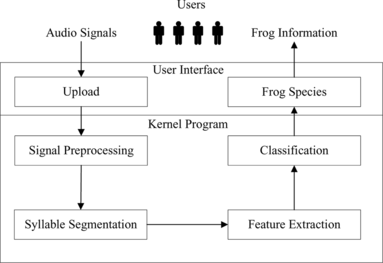
The architecture of the proposed frog call identifier can be divided into four main modules, including signal preprocessing, syllable segmentation, feature extraction, and classification modules, as illustrated in Figure 1. Undesirable information is first removed from the raw input signals in order to preserve the desired characteristics of frog call during the signal preprocessing stage. The resulting signal is then segmented by the syllable segmentation method and the segmented syllables are further processed during the feature extraction stage to produce meaningful parameters for the classifier.

FIGURE 1 Architecture of the intelligent frog call identifier.

Signal Preprocessing

The recorded sound signal is resampled at 16 kHz frequency and saved as 16-bit mono format. The amplitude of each sound signal is normalized within the range [−1, 1] for the ease of further processing. Three techniques, including pre-emphasis (Buckwalter, Meghelli, and Friedman, 2006), denoise (Donoho, 1995), and discrete wavelet transform (DWT) (Lung, 2004) are applied in order to “purify” the data in the noisy environment.

The motivation of using a pre-emphasis technique is to compensate the high-frequency part that was suppressed during the recording of audio signal by using a sound production mechanism. A denoise filter is employed to remove the noise during the signal analysis, while the application of DWT is to resolve high-frequency and low-frequency components within a small and large time windows, respectively.

Adaptive Endpoint Detection Segmentation

A syllable is basically a sound that a frog produces with a single blow of air from the lungs. The rate of events in frog vocalization is so high that the separation of individual syllables is difficult in a natural environment due to reverberation. Once the syllables have been properly segmented (Janqua, 1994), a set of features can be collected to represent each syllable. In this work, we propose an adaptive endpoint detection segmentation method, in which a cleaner waveform can be obtained by accurately measuring the positions of two endpoints of the waveforms. It is observed that the peak amplitude of each individual syllable is located around the middle portion of each separate frog call. We thus extract the major portion of each syllable by trimming two sides of the peak to filter out the noise contained in the audio signal. Meanwhile, the parts of the filtered signal whose volumes fall below a predefined threshold are discarded and the longest continuous segment is extracted for the ease of the processing at the feature extraction stage.

The first part of the algorithm that trims two sides of the peak amplitude is summarized as follows:

1. Compute the amplitude of the input acoustic signal using iterative time-domain algorithm. We denote the amplitude a matrix S(a, t), where a represents amplitude value and t is the time sequence. Initially set n = 1.

2. Find a _n and t _n , such that S(a _n , t _n ) = max {S(|a|, t)}. Set the position of the nth syllable to be S(a _n , t _n ).

3. If |a _n | ≤a _threshold , stop the segmentation process. The a _threshold is the empirical threshold. This means that the amplitude of the nth syllable is too small and hence no more syllables need to be extracted.

4. Store the amplitude trajectories corresponding to the nth syllable in function A _n (τ), where τ =t _n  − ε,…, t _n ,…, t _n  + ε and ε is the empirical threshold of the syllable. The step is to determine the starting time t _n  − ε and the ending time t _n  + ε of the nth syllable around t _n .

5. Set S(a, (t _n  − ε,…, t _n  + ε)) = 0 to delete the area of nth syllable. Set n = n + 1 and go to (2) to find the next syllable.

The second part of the algorithm that extracts the longest continuous segment is summarized as follows:

1. The volume level of jth frame for the ith syllable can be expressed by

   where n is the number of empirical frame size, α _{i, t} represents the amplitude value at time t.

2. Initially set i = 1.

3. A volume sequence S _i is obtained via (1) and (2). The volume sequence of the ith syllable can be expressed by

   where ν _{i, k} is the volume level of the kth frame for the ith syllable, and {k} is a continuous integer sequence. Initially set k = 1.

4. Find a subset s in S _i , such that each frame of the subset s is greater than ν _threshold and s is the longest continuous segment. The value of ν _threshold is determined by the experiments.

5. The first and last elements in the subset s are regarded as the start and end-points of the filtered syllable.

6. Set i = i + 1. If there are unprocessed syllables, go to (3).

Feature Extraction

Seven well-known features widely applied in pattern recognition are employed in this work. They are spectral centroid, signal bandwidth, spectral roll-off, delta spectrum magnitude, spectral flatness, average energy, and mel-frequency cepstral coefficients. In addition, a new developed feature, a threshold-crossing rate, is proposed in this work to reduce the impact of the noises in the sound samples.

Spectral Centroid

The spectral centroid is the centerpoint of the spectrum and in terms of human perception, it is often associated with the brightness of the sound. Brighter sound is related to the higher centroid. The spectral centroid for signal syllable is calculated as

where x _n is the discrete Fourier transform (DFT) of a signal syllable for the nth sample and H is half the size of DFT. The DFT of each frame is expressed by

where k = 0,…, N − 1.

Signal Bandwidth

A signal bandwidth is defined as the width of the frequency band of a signal syllable around the centerpoint of the spectrum. The bandwidth is calculated as

Notably, the bandwidth of a syllable is calculated as average bandwidth of DFT frames of syllables.

Spectral Roll-Off

This feature measures the frame-to-frame spectral difference. In short, it shows the changes in the spectral shape. It is defined as the squared difference between the normalized magnitudes of a successive spectral distribution. A spectral roll-off frequency can be expressed by

where C is an empirical constant ranging between zero and one and x _n is the DFT of a signal syllable for the nth sample. The DFT of each frame is expressed in Equation (5).

Threshold-Crossing Rate

Traditionally, a zero-crossing rate is the number of time-domain zero-crossings in each individual syllable. A zero-crossing occurs when adjacent signals have different signs. A zero-crossing rate is closely related to a spectral centroid as they both can be used to derive the spectral shape of a syllable. The so-called threshold-crossing rate is adopted in this work to ignore the time-domain zero-crossings in each individual syllable produced by the noises. The threshold-crossing rate is defined as

where the function tsgn(·), which represents the threshold, is defined as

Here η is an empirical amplitude threshold set for the syllable.

Delta Spectrum Magnitude

A delta spectrum magnitude measures the difference in spectral shape. It is defined as the 2-norm of difference vector of two adjacent frame spectral amplitudes. It gives a higher value for syllables with a higher between-frame difference. The formula for a delta spectrum magnitude calculations is given as

Spectral Flatness

Spectral flatness measures the tonality of a sound. It gives a low value for noisy sounds and a high value for voiced sounds. The measure can also discriminate voiced sounds from unvoiced if they occupy the same frequency range. Spectral flatness is the ratio of a geometric to arithmetic mean of signal spectrum and it is given in dB scale as follows:

where is a geometric mean and is an arithmetic mean of the magnitude values of the spectral points X _i .

Average Energy

The average energy is defined as the sum of the eigen-energies time weights:

where f is the number of frames and is the sum of energy in the kth frame.

Mel-Frequency Cepstral Coefficients (MFCCs)

Mel-frequency cepstral coefficients are coefficients that represent audio. They are derived from a type of cepstral representation of the audio clip. The difference between the cepstrum and the MFCC is that in the MFCC, the frequency bands are positioned logarithmically on the mel scale such that the human auditory system's response can be approximated more closely than the linearly spaced frequency bands obtained directly from the fast Fourier transform (FFT) or discrete cosine transform (DCT). This can allow for better processing of data, such as in the application of audio compression. However, unlike the sonogram, MFCCs lack an outer ear model and cannot accurately represent perceived loudness. Mel-frequency cepstral coefficients are commonly derived as follows:

1. Take the Fourier transform of a windowed excerpt of a signal.

2. Map the log amplitudes of the spectrum obtained above onto the mel scale, using triangular overlapping windows.

3. Take the DCT of the list of mel log-amplitudes.

4. The MFCCs are the amplitudes of the resulting spectrum.

Classification

Three well-known machine-learning techniques (Vapnik, 1998)—the k-nearest neighbor classifier (kNN), the backpropagation neural network (BPNN), and the naive Bayes (NB)—classifier are used to classify the frog species in this work, while the spectral centroid, signal bandwidth, spectral roll-off, threshold-crossing rate, delta spectrum magnitude, spectral flatness, average energy, and MFCCs are taken as the input parameters to the classifier. These machine-learning techniques have been widely applied to various music sound analysis and music information retrieval problems in the literature.

k-Nearest Neighbor Classifier

k-nearest neighbor classifier (kNN) is a nonparametric approach for classification (Kelly and Davis, 1991). It does not require the priori knowledge such as priori probabilities and the conditional probabilities. It operates directly towards the samples and is categorized as an instance-based classification method.

kNN simply stores the representative training data. This algorithm assumes all the examples correspond to vectors in n-dimensional vector space. The neighbors of the examples are defined in terms of Euclidean (, 2005) distance function.

In the kNN, the k-nearest samples in the training data set are found, for which the majority class is determined. This algorithm can be summarized as follows. Given an unknown feature vector x and a distance measure, then:

1. Identify the K nearest neighbors out of N training vectors, irrespective of the class label, where K is chosen to be odd.

2. Out of these K samples, identify the number of vectors k _i that belong to the class c _i , i = 1, 2, 3,…, M.

3. x is determined to belong to the class c _i with the maximum number k _i of samples.

The distance measure for features is of critical importance for a kNN classifier. The Euclidian distance function is the most widely used in kNN. It is defined as

where a = (a ₁, a ₂,…, a _n ) and b = (b ₁, b ₂,…, b _n ) are two points in the n-dimensional space.

Backpropagation Neural Network

A neural network (Haykin, 1994) is able to recognize patterns and generalize from them. An essential feature of this technology is that it improves its performance on a particular task by gradually learning a mapping between inputs and outputs. Generalization is used to predict the possible outcome for a particular task. This process involves two phases known as the training phase and the testing phase. Backpropagation (BP) neural network is one of the neural networks most in common use. Figure 2 shows an example of a BP neural network. In BP the learning procedure basically follows that of a traditional feed-forward neural network. However, there are two main differences. The first difference is the use of the activation function of the hidden unit y _j , and the second is that the gradient of the activation function is contained.

FIGURE 2 A backpropagation neural network.

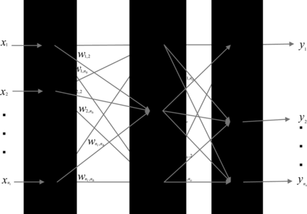
A BP neural network consists of several layers of nodes, including an input layer, one or more hidden layers, and an output layer. Each node in a layer receives its input from the output of the previous layer nodes. The connections between nodes are associated with synaptic weights that are iteratively adjusted during the training process. Each hidden and output node is associated to an activation function. Several functions can be used as activation functions, but the most common choice is the sigmoid function:

Provided that the activation function of the hidden layer nodes is nonlinear, a BP neural network with an adequate number of hidden nodes is able to approximate every nonlinear function. The adjustment of the synaptic weights in an error BP algorithm consists of four steps:

1. The network is initialized by assigning random values to synaptic weights.

2. A training pattern is fed and propagated forward through the network to compute an output value for each output node.

3. Actual outputs are compared with the expected outputs.

4. A backward pass through the network is performed, changing the synaptic weights on the basis of the observed output errors.

Steps (2) through (4) are iterated for each pattern in a training set until convergence.

In the case of neural networks with a single hidden layer as shown in Figure 2, the forward propagation step is carried out as follows:

where x _j is the jth input from the input layer, and w _jk is the weight of the connections between input x _j and the kth node at the hidden layer. To compute the outputs of the hidden layer, these weighted sums are passed to the activation function:

where g _{n h  + 1} denotes the output of the bias node at the hidden layer. Then the network outputs are computed by

After the forward propagation, the estimated output o _l of the lth node at the output layer is compared with the expected output y _l and a mean quadratic error for the current pattern is derived by

In the BP step, all the synaptic weights are adjusted in order to follow a gradient descent on the error surface. For the connection weight between the kth node at the hidden layer and the lth node at the output layer, z _kl , is adjusted by

where η denotes the learning rate and

The weight w _jk of the connection between the kth node at the hidden layer and the jth input is adjusted by

where is computed by

The network training is iterated until a given condition is met.

NB Classifier

The NB classifier is a probabilistic method for classification. It can be used to determine the probability that an example belongs to a class given the values of variables. The simple NB classifier is one of the most successful algorithms in many classification domains. In spite of its simplicity, it is shown to be competitive with other complex approaches, especially in text categorization and content-based filtering.

Classification is then done by applying the Bayes rule to compute the probability of C given the particular instance of X ₁,…, X _n ,

As variables are considered independent given the value of the class, the conditional probability can be calculated as follows:

This equation is well suited for learning from data, since the probabilities P(C = c _i ) and P(X _k  = x _k  | C = c _i ) may be estimated from training data. The result of the classification is the class with highest probability.

Web Interface Design

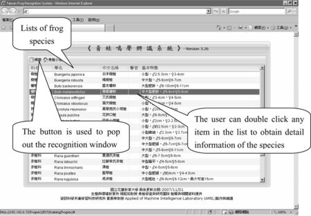
As Figure 3 shows, the online frog recognition web interface includes two main windows. The first window is the lists of frog species, which is located at the center of the screen. The users can press the button to pop out the recognition window. The users can double-click any item on the list to get more information for that corresponding species.

FIGURE 3 The web interface of the online frog recognition system.

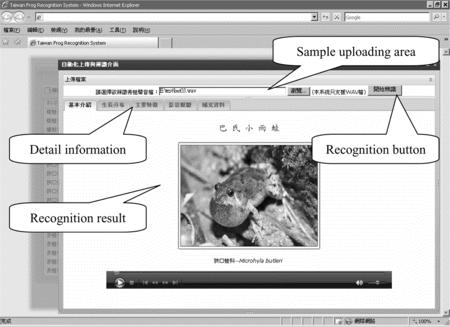
The second window is the recognition window, which includes two main parts. The first part is the sample file uploading area, which is located at the upper portion of the window. The users can press the recognition button to activate the classification process when the sample file is provided. As given in Figure 4, the center area of the window displays frog's species and their characteristics, e.g., photos, which can be adopted by the users to collect the information for the frogs.

FIGURE 4 Recognition result.

EXPERIMENTAL RESULTS

In this work, a database that consists of five frog species as listed in Table 1 was used in the experiments to verify the effectiveness of the proposed frog call identifier. Fifteen frog species are evenly distributed in 75 wave files and each file contains only one species. The resampling frequency is 16 kHz and each sample is digitized in 16-bit mono. Each acoustic signal is first segmented into a set of syllables. The value of the threshold level used in the adaptive endpoint detection segmentation method is set to 35% of the maximum volume of the input sequence. The frame size and overlapping size are 512 and 256 samples, respectively. In Table 2, the total number of samples is 2080 syllables, spanned from 75 wave files. The number of training syllables is 1401 and that of holdout syllables is 679. That is, about one-third of the syllables are used for holdout and the rest are used for training.

TABLE 1 Frog Species for Family Microhylidae and Phacophoridae

Family	Scientific name	Common name
Microhylidae	Microhyla heymonsi	Heymonsi narrow-mouthed toad
	Kaloula pulchra	Malaysian narrow-mouthed toad
	Microhyla butleri	Butler's rice frog
	Microhyla ornate	Ornate rice frog
	Microhyla steinegeri	Stejneger's paddy frog
Phacophoridae	Buergeria japonica	Japanese tree frog
	Buergeria robusta	Brown tree frog
	Chirixalus eiffingeri	Eiffingers tree frog
	Chirixalus idiootocus	Meintein tree frog
	Polypedates megacephalus	White-lipped tree frog
	Rhacophorus arvalis	Rhacophorus arvalis
	Rhacophorus aurantiventris	Orange-belly green tree frog
	Rhacophorus moltrechti	Moltrechtis green tree frog
	Rhacophorus prasinatus	Emerald green tree frog
	Rhacophorus taipeianus	Taipei green tree frog

TABLE 2 Number of Syllables

	Syllable
Family	Training	Testing	Total
Microhylidae	483	251	734
Phacophoridae	918	428	1346
Total	1401	679	2080

The following classification accuracy rate is used to examine the performance of the proposed work:

where N _C is the number of syllables that were recognized correctly and N _T is the total number of testing syllables.

The average cost of each classifier is defined as

where T is the cost of an classifier, and N is the total number of syllables for classification.

We first took MFCCs as the input parameters to the classifier because MFCCs are composed of 13 individual elements. Then a set of the seven above-introduced features, including spectral centroid, signal bandwidth, spectral roll-off, threshold-crossing rate, delta spectrum magnitude, spectral flatness, and average energy is used as the input parameters to the classifiers. The classification results for the three classifiers, including kNN, BPNN, and NB, are listed in Table 3. It can be observed that the MFCCs outperform the combination of the seven features in term of the accuracy rate, although more computation time is required for the MFCCs. Moreover, kNN slightly outperforms the other two classifiers, BPNN and NB.

TABLE 3 Accuracy Rates ofkNN, BPNN, and NB Classifiers with Different Combination of the Input Parameters

	Classifier
	kNN		BPNN		NB
	Accuracy	Average	Accuracy	Average	Accuracy	Average
Input parameters	rate	cost	rate	cost	rate	cost
MFCCs	0.88365	1.407769	0.85272	1.365128	0.76878	1.257871
A set of seven features	0.93814	2.391338	0.88218	2.529845	0.86009	2.335718

CONCLUSION AND THE FUTURE WORK

An intelligent frog call identifier is proposed in this work to effectively recognize the 15 frog species based on the recorded audio samples. An adaptive endpoint detection segmentation method is employed to separate the syllables from raw sound samples. Eight features, including spectral centroid, signal bandwidth, threshold-crossing rate, spectral roll-off, delta spectrum magnitude, spectral flatness, average energy, and mel-frequency cepstral coefficients, are extracted from the syllables to serve as two sets of the input parameters for three well-known classifiers, including kNN, BPNN, and NB.

A series of experiments were performed to verify the effectiveness of the proposed algorithms. The classification accuracy for kNN, BPNN, and NB classifiers based on a set of the seven features, including spectral centroid, signal bandwidth, spectral roll-off, threshold-crossing rate, delta spectrum magnitude, spectral flatness, and average energy, is up to 88.36%, 85.27%, and 76.87%, respectively; whereas the classification accuracy for the three classifiers based on the feature of MFCCs is up to 93.81%, 88.21%, and 86.00%, respectively. It can be inferred from the experimental results that the proposed online recognition system is adequate for the identification of frog sounds.

The authors would like to thank the National Science Council of Taiwan (contract no. NSC 96-2628-E-026-001-MY3) and the Forestry Bureau Council of Agriculture of Taiwan (contract no. 96-FM-02.1-P-19(2)) for financially supporting this research.

REFERENCES

- Beritelli , F. 2000 . Robust word boundary detection using fuzzy logic . Electronics Letters 36 ( 9 ): 846 – 848 .
- Buckwalter , F. M. , and J. Friedman . 2006 . Phase and amplitude pre-emphasis techniques for low-power serial links . IEEE Journal of Solid-State Circuits 41 ( 6 ): 1391 – 1399 .
- Donoho , L. 1995 . De-noise by soft-thresholding . IEEE Transactions on Information Theory 41 ( 3 ).
- Duellman , W. E. and L. Trueb . 1986 . Biology of Amphibians . New York : McGraw-Hill Book Company .
- Erdöl , N. , C. Castelluccia , and A. Zilouchian . 1993 . Recovery of missing speech packets using the short-time energy and zero-crossing measurements . IEEE Trans. on Speech and Audio Processing 1 ( 3 ): 295 – 303 .
- Fagerlund , S. 2007 . Bird species recognition using support vector machines . EURASIP Journal on Applied Signal Processing 1 : 64 .
- Guodong , G. and Z. Li . 2003 . Content-based classification and retrieval by support vector machines . IEEE Transactions on Neural Networks 14 : 209 – 215 .
- Harma , A. 2003 . Automatic identification of bird species based on sinusoidal modeling of syllables . International Conference on Acoustic Speech Signal Process 5 : 545 – 548 .
- Haykin , S. 1994 . Neural Networks: A Comprehensive Foundation . New York : Macmillan College Publishing Company .
- Janqua , J.-C. 1994. A Robust algorithm for word boundary detection in the presence of noise. IEEE Trans. on Speech and Audio Processing 2(3):406–412.
- Kelly , J. D. and L. Davis . 1991 . Hybridizing the genetic algorithm and the K nearest neighbors classification algorithm . 4th International Conference on Genetic Algorithms and Applications 377 – 383 .
- Kogan , J. A. and D. Margoliash . 1998 . Automated recognition of bird song elements from continuous recordings using DTW and HMMs . Journal of the Acoustical Society of America 103 ( 4 ): 2185 – 2196 .
- Liu , L. , J. He , and G. Palm . 1997 . Effects of phase on the perception of intervocalic stop consonants . Speech Communication 22 : 403 – 417 .
- Lung , S.-Y. 2004 . Feature extracted from wavelet eigenfunction estimation for text independent speaker recognition . Pattern Recognition 37 : 1543 – 1544 .
- Mitrovic , D. and M. Zeppelzauer . 2006 . Discrimination and retrieval of animal sounds . In: Proceedings of the IEEE Multimedia Modelling Conference , Beijing , China .
- Peterson , M. R. , T. E. Doom , and M. L. Raymer . 2005 . GA-facilitated kNN classifier optimization with varying similarity measures . IEEE Congress on Evolutionary Computation 3 : 2514 – 2521 .
- Somervuo , P. , A. Härmä , and S. Fagerlund . 2006 . Parametric representations of bird sounds for automatic species recognition . IEEE Transactions on Audio, Speech and Language Processing 14 ( 6 ): 2252 – 2263 .
- Tyagi , H. , R. M. Hegde , H. A. Murthy , and A. Prabhakar . 2006 . Automatic identification of bird calls using spectral ensemble average voiceprints . In: Proceedings of the 13th European Signal Processing Conference , Florence , Italy .
- Vapnik , V. 1998 . Statistical Learning Theory . New York : Wiley .
- Vilches , E. , I. A. Escobar , E. E. Vallejo , and C. E. Taylor . 2006 . Data mining applied to acoustic bird species recognition . In: Proceedings of the 18th International Conference on Pattern Recognition 3 : 400 – 403 , Hong Kong .