CONFIDENCE METRICS FOR ASSOCIATION RULE MINING

Abstract

We propose a simple, novel, and yet effective confidence metric for measuring the interestingness of association rules. Distinguishing from existing confidence measures, our metrics really indicate the positively companionate correlations between frequent itemsets. Furthermore, some desired properties are derived for examining the goodness of confidence measures in terms of probabilistic significance. We systematically analyze our metrics and traditional ones, and demonstrate that our new algorithm significantly captures the mainstream properties. Our approach will be useful to many association analysis tasks where one must provide actionable association rules and assist users to make quality decisions.

Measurements of interestingness are very important for association rule mining. This is partly because the search space for association rules is usually very large and we need to confine our interests within a certain scope. Moreover, the number of association rules extracted is often very large as well, too large for human beings to deal with directly (Zhang and Zhang, 2002; Zhang, Wu, Zhang, and Lu, 2008). We have to prune those uninteresting rules according to their interestingness. In applications such as evaluating the quality and ranking the association rules extracted, we also need interestingness measures. Therefore, much research has been dedicated to defining appropriate measures of interestingness from various angles and in many disciplines, such as statistics, information theory, machine learning, and data mining.

The interestingness of an association rule generally includes validity, novelty, usefulness, and simplicity. However, it is really hard to capture all of these factors in a measurement at the same time. Common methods for association rules use statistical measures. Specific applications may have their own objective functions and constraint conditions on some numerical characteristics, such as time, distance, cost, and profit. Templates can also be used in certain applications to describe the interestingness of an association rule. That is, an association rule is interesting only if it matches a restrictive template.

According to Silberschatz and Tuzhilin (1996) and Zhang and Zhang (2002), measures of interestingness can be divided into two categories: objective and subjective. Objective measures define interestingness of a pattern in terms of the pattern structure and the underlying data used to mine the pattern. Subjective measures depend not only on the structure and data, but also on the user beliefs regarding relationships in the data. One of the arguments in favor of subjective measures is that a pattern that is interesting to a user may be of no interest to another user. In Silberschatz and Tuzhilin (1996), subjective measures are further classified into unexpected and actionable. In our opinion, unexpectedness is more important than actionability, because actionability is more ambiguous, it is hard to formally capture actionability, most unexpected patterns are actionable, and unexpectedness is intrinsic for interestingness. Silberschatz and Tuzhilin (1996) also uses unexpectedness to define the measure of subjective interestingness, based on a given system of beliefs, although it claims that the actionability is the major concept.

For an association rule A → B, the interestingness is measured by both the support supp(A ∪ B) and the confidence supp(A ∪ B)/supp(A) in Agrawal, Imielinski, and Swami (1993), where supp(X) is the support of X. While the support is commonly held, constructing suitable confidence metrics has become the center problem in interestingness analysis.

In Dong and Li (1998), it is believed that the neighborhood of a rule should be taken into account when considering unexpectedness of the rule. That is, interestingness of a rule should depend on the confidence fluctuation and rule density in the neighborhood of the rule. Thus, distance between rules and neighborhood of a rule are introduced. Some expected tendencies of changes resulting from the structure of the rules are used when considering the unexpectedness of changes.

Some of other common interestingness measures for association rule mining are listed:

	Interest Factor (Brin, Motwani, and Silverstein, 1997; Silverstein, Brin, and Motwani, 1998): It is a non-negative real number, with value 1 corresponding to the statistical independence.
	Pearson's correlation coefficient: It is ranged between −1 to 1. If A and B are independent, then φ(A → B) = 0.
	Cosine similarity:
	Odds ratio:
	Rule-interest (Piatetsky-Shapiro, 1991):
	Conviction (Brin, Motwani, Ullman, and Tsur, 1997):
	Certainty factor (Wu, Zhang, and Zhang, 2004; Zhang and Zhang, 2002):
	Laplace measure: Obviously, it is very similar to the confidence.
	J-measure (Wang, Tay, and Liu, 1998):

Although numerous metrics have been proposed to measure the interestingness of association rules, we still need to look for a more suitable one for a specific application. The best metric for a given situation is usually unknown. In other words, there is no measure that is always better than others in all cases. Many of the measures provide similar information about the interestingness of a pattern. Some of them are even conflicting. This is because interestingness is so complicated that we cannot integrate all its factors, such as usability, unexpectedness, and soundness, into a function or a formula. Each measure inevitably has its own relatively focused contribution to the interestingness. Because an association rule X → Y is asymmetric between X and Y, we think that the interestingness measure of X → Y should be asymmetric as well.

PRELIMINARIES

This section recalls some concepts required for association rule mining (Yan, Zhang, and Zhang, 2007; Zhang and Zhang, 2002), which briefly states the challenges and outlines the research into genetic algorithm-based mining techniques (Yan, Zhang, and Zhang, 2005).

I = {i ₁, i ₂,…, i _m } is a set of literals, or items. For example, goods such as milk, sugar, and bread for purchase in a store are items; and A _i  = v is an item, where v is a domain value of attribute, A _i , in a relation, R(A ₁,…, A _n ).

X is an itemset if it is a subset of I. For example, a set of items for purchase from a store is an itemset; and a set of A _i  = v is an itemset for the relation R(PID, A ₁, A ₂,…, A _n ), where PID is a key.

D = {t _i , t _i+1,…, t _n } is a set of transactions called the transaction database, where each transaction t has a tid and a t-itemset: t = (tid, t-itemset). For example, the shopping cart of a customer going through checkout is a transaction; and a tuple (v ₁,…, v _n ) of the relation R(A ₁,…, A _n ) is a transaction.

A transaction, t, contains an itemset, X, if and only if (iff) for all items, i ∊ X, i is in t-itemset. For example, a shopping cart contains all items in X when going through checkout; and for each A _i  = v _i in X, v _i occurs at position i in the tuple, (v ₁,…, v _n ).

There is a natural lattice structure on the itemsets, 2 ^I , namely, the subset/superset structure. Certain nodes in this lattice are natural grouping categories of interest (some with names)—for example, items from a particular department; clothing, hardware, furniture,…, and within clothing; children's, women's, and men's, toddler's, and so on.

An itemset, X, in a transaction database, D, has a support, denoted as supp(X) (we also use p(X) to stand for supp(X)), that is, the ratio of transactions in D contain X. Or

where X(t) = {t in D | t contains X}.

An itemset, X, in a transaction database, D, is called a large (frequent) itemset if its support is equal to, or greater than, a threshold of minimal support (minsupp), which is given by users or experts.

An association rule is an implication X → Y, where itemsets X and Y do not intersect.

Each association rule has two quality measurements: support and confidence, defined as:

	the support of a rule X → Y is the support of X ∪ Y, where X ∪ Y means both X and Y occur at the same time;
	the confidence of a rule X → Y is con f(X → Y) as the ratio: |(X ∪ Y)(t)|/|X(t)| or supp(X ∪ Y)/supp(X),

that is, support = frequencies of occurring patterns; confidence = strength of implication.

Support-confidence framework (Agrawal et al., 1993): Let I be the set of items in database D, X, Y ⊆ I be itemsets, X ∩ Y = , p(X) ≠ 0 and p(Y) ≠ 0. Minimal support (minsupp) and minimal confidence (minconf) are given by users or experts. Then X → Y is a valid rule if:

1. supp(X ∪ Y) ≥ minsupp,

2. ,

where “con f(X → Y)” stands for the confidence of the rule X → Y.

Mining association rules can be broken down into the following two subproblems:

1. Generating all itemsets that have support greater than, or equal to, the user-specified minimum support, that is, generating all large itemsets.

2. Generating all the rules that have minimum confidence in the following naive way: for every large itemset X, and any B ⊂ X, let A = X − B. If the confidence of a rule A → B is greater than, or equal to, the minimum confidence (or supp(X)/supp(A) ≥ mincon f), then it can be extracted as a valid rule.

To demonstrate the use of the support-confidence framework, we illustrate the process of mining association rules by an example as follows.

Example 1

Suppose we have a market basket database from a grocery store, consisting of n baskets. Let us focus on the purchase of tea (denoted by t) and coffee (denoted by c).

When supp(t) = 0.25 and supp(t ∪ c) = 0.2, we can apply the support-confidence framework for a potential association rule t ⇒ c. The support for this rule is 0.2, which is fairly high. The confidence is the conditional probability that a customer who buys tea also buys coffee, i.e., con f(t ⇒ c) = supp(t ∪ c)/supp(t) = 0.2/0.25 = 0.8, which is very high. In this case, we would conclude that the rule t → c is a valid one.

A NEW CONFIDENCE METRICS

In terms of the probability theory, the confidence of a rule X → Y is the conditional probability that a tuple contains Y, given that it contains X. If X acts positively on Y, this conditional probability p(Y | X) should be larger than p(Y), the probability that a tuple contains Y. On the other hand, if X is negative to Y, the conditional probability p(Y | X) should be less than the probability p(Y), that is, we have the following proposition.

Proposition 1

There are three cases of relationship between X and Y as follows according to the conditional probability p(Y | X):

1. If p(Y | X) = p(Y), then Y and X are independent.

2. If p(Y | X) > p(Y), then Y is positively dependent on X.

3. If p(Y | X) < p(Y), then Y is negatively dependent on X.

Therefore, for any association rule X → Y of potential interest, we can reasonably require that the confidence con f(X → Y) should be distributed between supp(Y) and 1 if X is positive to Y, or between 0 and supp(Y) if X is negative to Y. Given a user-specified and normalized minimum confidence, rmincon f ∊ [−1, 1], we first transform it to mincon f ∊ [supp(Y), 1] if 0 ≤rmincon f ≤ 1, or mincon f ∊ [0, supp(Y)] if −1 ≤rmincon f < 0, such that 1, 0, and −1 are mapped to 1, supp(Y), and 0, respectively, as shown in Figure 1.

FIGURE 1 Mapping from rcon f to con f.

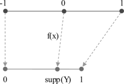
This transformation from rmincon f to mincon f can be obtained by constructing the following mapping f:

i.e.,

Then, the confidence of an interesting rule X → Y needs to satisfy

i.e.,

Thus,

We refer to the left side of Inequality (2) as the relative confidence, because it is a confidence measure relative to supp(Y). Formally, we define the relative confidence for a rule X → Y as

If supp(X) = 0, then supp(X ∪ Y) = 0 for any itemset Y and it is meaningless to discuss the confidence of rule X → Y in the context of association rule mining. Hence, we consider the rule is uninteresting, and define rcon f(X → Y) = 0 when supp(X) = 0.

If 1 −supp(Y) = 0, i.e., supp(Y) = 1, then Y occurs in every tuple, and supp(X ∪ Y) = supp(X) holds for any itemset X. Hence we have supp(X ∪ Y) ≥ supp(X)supp(Y), and

Therefore, we define

If supp(Y) = 0, then supp(X ∪ Y) = 0 for any itemset X. We have con f(X → Y) = 0. Thus, we define rcon f(X → Y) = −1 when supp(Y) = 0.

When supp(X) = 0, supp(Y) = 0, or supp(Y) = 1, rule X → Y is referred to as a trivial rule. For association rule mining, trivial rules are not interesting. They should be excluded from the output of our algorithm.

The relative confidence defined by Equation (3) is, in fact, similar to the probability ratio proposed in Wu, Zhang, and Zhang (2004) and Zhang and Zhang (2002).

Now we restate the second subproblem of generating association rules for a given threshold of the relative confidence rmincon f ∊ [0, 1]:

1. Generate all rules that satisfy the constraint of relative confidence. That is, for any frequent itemset F, and any X ⊂ F, let Y = F − X. Rule X → Y is generated if and only if rcon f(X → Y) ≥ rmincon f holds.

The rules generated by (2′) represent the positive association between itemsets. Similarly, when given rmincon f ∊ [−1, 0), what we want to mine is the negative relationship between itemsets. The second subtask becomes:

1. For any frequent itemset F, and any X ⊂ F, let Y = F − X. Rule X → Y is generated if and only if rcon f(X → Y) ≤ rmincon f holds.

We now design a procedure for the second subproblem of mining association rules. For every frequent itemset S, Procedure 1 finds all nonempty subsets of S. For every such subset X, output a rule of the form X → (S − X) if it is nontrivial and its relative confidence satisfies the condition about the minimum relative confidence rmincon f.

Procedure 1

RCONF

Table

//find all interesting association rules for a frequent itemset

Input: S: a given frequent itemset;

rmincon f: the minimum relative confidence;

Output: interesting association rules;

begin

for any nonempty subset X ⊂ S do

begin

let Y ← S − X;

if supp(X)supp(Y)(1 −supp(Y)) ≠ 0 then

begin

if rmincon f ≥ 0 then

let ;

else

let ;

if(rcon f ≥ rmincon f ≥ 0) then

output positive associationX → Y ;

else if(rcon f ≤ rmincon f < 0) then

output negative associationX → Y ;

end

end

end

This procedure prunes all the trivial rules and those rules that fail to meet the relative confidence requirement, by simply calculating the relative confidence for each rule within itemset S and judging whether it is interesting. Both positive and negative relationships between itemsets can be found by specifying a positive or negative threshold of the minimum relative confidence, respectively. The procedure assumes that we have kept tracks of supports for each subset of the frequent itemset S.

Procedure 1 is to find all interesting association rules for a given frequent itemset, which is the same as the traditional Apriori algorithm (Agrawal et al., 1993) except using different measures of interestingness. Both measures of interestingness can be computed in a constant time. Hence, both procedures have the same magnitude of time complexity.

EXPERIMENTS

In order to demonstrate the effectiveness of Procedure 1, we apply two datasets to our algorithm, and we only consider the positive relationship between itemsets here, that is rmincon f > 0. One of the datasets is the Mushroom database from UCI at http://www.ics.uci.edu/\~mlearn. Table 1 and Figures 2 and 3 give the results when con f and rcon f are used for computations, respectively, and the rule length is fixed to 2. The number of association rules generated are calculated at nine sample points where the thresholds are set to 90%, 80%, 70%, 60%, 50%, 40%, 30%, 20%, 10%, respectively. Nine different values of the minimum supports, ranged isometrically from 10% to 90%, are also used, respectively. It has been shown that many association rules are pruned by using the relative confidence.

FIGURE 2 Results from the mushroom dataset when minsupp = 20%.

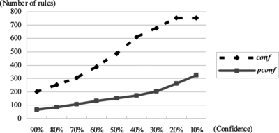
FIGURE 3 Results from the mushroom dataset when minsupp = 40%.

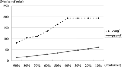
TABLE 1 Results Based on the Mushroom Dataset

Minimum	con f.	90%	80%	70%	60%	50%	40%	30%	20%	10%
minsupp	con f	277	354	437	569	760	1001	1217	1439	1526
=10%	rcon f	115	138	172	210	247	293	349	499	652
minsupp	con f	201	254	305	387	486	609	676	752	1526
=20%	rcon f	68	86	107	132	153	173	204	262	325
minsupp	con f	110	145	163	211	261	306	326	326	326
=30%	rcon f	20	30	40	49	60	72	87	110	130
minsupp	con f	81	104	111	135	165	194	194	194	194
=40%	rcon f	15	18	24	29	35	42	48	54	61
minsupp	con f	42	52	52	66	82	82	82	82	82
=50%	rcon f	9	9	9	9	10	11	12	12	15
minsupp	con f	23	28	28	36	36	36	36	36	36
=60%	rcon f	2	2	2	2	2	2	3	3	4
minsupp	con f	16	20	20	20	20	20	20	20	20
=70%	rcon f	2	2	2	2	2	2	3	3	4
minsupp	con f	15	18	18	18	18	18	18	18	18
=80%	rcon f	2	2	2	2	2	2	2	2	2
minsupp	con f	8	8	8	8	8	8	8	8	8
=90%	rcon f	2	2	2	2	2	2	2	2	2

Figures 2 and 3 only show the number of association rules generated from the Mushroom dataset when mimsupp = 20% and 40%, respectively.

In Table 2, we have similar results based on the WisconsinBreastCancer dataset from UCI. This dataset has 699 rows and 11 columns. The same sampling schema as used in Table 1 is adopted, and a similar relationship between the traditional confidence and the relative confidence can be drawn from Table 2. For example, Figure 4 shows the number of association rules generated from the breast cancer dataset when mimsupp = 20%, which is similar to Figures 2 and 3. We shall give the details of our analysis on these results in the next section. Some of the properties about the relative confidence are attractive and useful for association rule mining.

FIGURE 4 Results from the breast cancer dataset when minsupp = 20%.

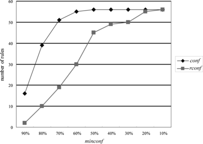
TABLE 2 Results Based on the Breast Cancer Dataset

Minimum	con f.	90%	80%	70%	60%	50%	40%	30%	20%	10%
minsupp	con f	28	66	89	99	106	106	125	142	154
=10%	rcon f	5	16	31	53	71	81	88	97	121
minsupp	con f	23	50	62	66	67	67	74	78	78
=20%	rcon f	4	15	26	40	55	59	61	66	74
minsupp	con f	16	39	51	55	56	56	56	56	56
=30%	rcon f	2	10	19	30	45	49	50	55	56
minsupp	con f	16	39	51	55	56	56	56	56	56
=40%	rcon f	2	10	19	30	45	49	50	55	56
minsupp	con f	13	20	24	28	28	28	28	28	28
=50%	rcon f	2	8	13	17	22	22	23	28	28
minsupp	con f	2	2	4	4	4	4	4	4	4
=60%	rcon f	0	1	2	2	2	2	3	4	4
minsupp	con f	2	2	4	4	4	4	4	4	4
=60%	rcon f	0	1	2	2	2	2	3	4	4
minsupp	con f	0	0	0	0	0	0	0	0	0
≥70%	rcon f	0	0	0	0	0	0	0	0	0

ANALYSIS

This section first presents some properties a good interestingness measure should have for association rule mining, then analyzes the relative confidence based on our computations.

Desirable Properties of Measure

Let X → Y is an association rule. Table 3 shows the correlation between itemsets X and Y, where, s ₁₁ = supp(X ∪ Y), s ₁₀ = supp(X ∪ ¬ Y), s ₀₁ = supp(¬ X ∪ Y), and s ₀₀ = supp(¬ X ∪ ¬ Y).

TABLE 3 A2 × 2 Contingency Table for ItemsetsA and B

	Y	¬Y
X	s 11	s 10	s 1+
¬X	s 01	s 00	s 0+
	s +1	s +0	s ++

Namely, based on the supports of itemsets, the correlation between X and Y can be described by the following matrix:

Consider measures that are defined over M for association rule X → Y. Then a measure can be viewed as an operator, O, which transforms matrix M into a scalar interestingness. Given a measure O, Piatetsky-Shapiro (1991) gave three desirable properties that measure what O should have. These three key properties can be presented formally as follows.

Property 1

(Independence)] O(M) = 0 if and only if det(M) = 0.

Property 1 is equivalent to the well-known requirement that O(M) = 0 iff X and Y are statistically independent. In fact, det(M) = 0 iff

Therefore, if and only if det(M) = 0, we have:

i.e., X and Y are statistically independent.

Property 2

(Increasing Monotonicity with supp(X ∪ Y))] Let

where k is a positive increment to the support of X ∪ Y. Then O(M′) > O(M).

Property 2 says that the measure will monotonically increase if supp(X ∪ Y) increases, and both supp(X) and supp(Y) remain the same.

Property 3

(Decreasing Monotonicity Against supp(X) or supp(Y))] Let

where k is a positive increment to the support of X or Y. Then O(M″) < O(M).

Property 3 indicates that the measure will monotonically decrease if supp(X) (or supp(Y)) increases, and both supp(X ∪ Y) and supp(Y) (or supp(X)) remain the same.

These three key properties can be expanded with the following four properties as well.

Property 4

(Decreasing Monotonicity Against supp(X) and supp(Y))] Let

where k ₁ and k ₂ are positive increments to supports of X and Y, respectively. Then O(M ⁽³⁾) < O(M).

Property 4 means that the measure will monotonically decrease if both supp(X) and supp(Y) increase, and supp(X ∪ Y) remains the same. Property 4 can be derived directly from Property 3, because

Property 5

(Increasing Monotonicity with Invariant Difference of supp(X ∪ Y) and supp(X) (or supp(Y)). Let

where k is a positive increment to the support of X ∪ Y. Then O(M ⁽⁴⁾) > O(M).

Property 5 says that the measure will monotonically increase if supp(X ∪ Y) increases, and both supp(X) (or supp(Y)) and the difference between supp(Y) (or supp(X)) and supp(X ∪ Y) remain the same.

Property 6

(Increasing Monotonicity with Invariant Ratio of supp(X ∪ Y) Over supp(Y)). Let

where k ₁ and k ₂ are positive increments to supports of X ∪ Y and ¬ X ∪ Y, respectively, and . Then O(M ⁽⁵⁾) ≥ O(M).

Property 6 says that the measure will not decrease if supp(X ∪ Y) increases, and both supp(X) and the ratio of supp(X ∪ Y) over supp(Y) remain the same.

Property 7

(Increasing Monotonicity with Invariant Ratio of supp(X ∪ Y) Over supp(X)). Let

where k ₁ and k ₂ are positive increments to supports of X ∪ Y and X ∪ ¬ Y, respectively, and . Then O(M ⁽⁶⁾) ≥ O(M).

Property 7 says that the measure will not decrease if supp(X ∪ Y) increases, and both supp(Y) and the ratio of supp(X ∪ Y) over supp(X) remain the same. In fact, the ratio of supp(X ∪ Y) over supp(X) is con f(X → Y).

Following are some other properties given in Tan, Kumar, and Srivastava (2002), which we do not think are necessary for association rule mining. But we still present them below as reference.

Property 8

[Property 8 (Symmetry)] O(M ^T ) = O(M), where M ^T is the transposed matrix of M.

Property 8 means that the measure is symmetric for X and Y. We suggest that this symmetry property is not desirable for association rules mining.

Property 9

(Scaling Invariance)] Let

where k ₁ and k ₂ are positive scaling factors. Then O(M·N) = O(M) and O(N·M) = O(M).

Property 9 means that scaling two rows (and columns) in M by k ₁ and k ₂, respectively, makes the measure unchanged.

Property 10

[Property 10 (Anti-Symmetry)] Suppose that measure O is normalized, i.e., its value ranges between −1 and 1. Let

Then O(M·S) = −O(M) and O(N·M) = −O(M).

Property 10 means that the measure is anti-symmetric between X and ¬ X (or between Y and ¬ Y).

Property 11

(Inversion Invariance)] Let S be the same as that in Property 10. Then O(S·M·S) = O(M).

Property 11 is a special case of Property 10 when measure O is normalized.

Property 12

(Null Invariance)] Let

where k is a positive constant. Then O(M + C) = O(M).

Property 12 implies that tuples that do not contain itemsets X and Y do not influence the interestingness measure for X → Y. These measures that satisfy Property 12 are suitable for positive association rule mining in sparse datasets.

Analysis on Confidence

From definition of the traditional confidence, we know that con f(X → Y) should be located in an interval of [supp(Y), 1], if X → Y is of potential interest. This means that determination of the minimum confidence should be dependent on supp(Y). Consequently, it is unsuitable to ask users to provide a fixed minimum confidence before the mining job. On the other hand, since Procedure 1 uses the relative confidence, instead of the traditional one, it can avoid the problem above by specifying a minimum relative confidence in interval [0, 1], which is independent on the support for the consequence of any rule. Our experiments also demonstrate the effectiveness of Procedure 1. Followings are some of our observations and propositions:

1. Procedure 1 usually outputs much smaller amounts of association rules than the classical algorithm does. Those additional rules generated by using con f, in fact, are not interesting for a given threshold of the relative confidence.

2. The change speed of the number of rules generated by using rcon f in [0, 1] is slower than that by using con f.

3. If mincon f < minsupp, the number of generated rules for this mincon f by using con f is the same as that with mincon f = minsupp.

4. The more rules are extracted by using con f, the more rules are pruned by using rcon f.

Based on the above observations, we have the following proposition.

Proposition 2

Given a threshold minsupp and a rule X → Y such that supp(X → Y) ≥ minsupp, we have

if Y is positively dependent on X.

Proof

In fact, if rule X → Y is extracted by using con f, we have

that is, supp(X ∪ Y) ≥ minsupp, according to the definition. Hence,

Since Y is positively dependent on X, by Proposition 1 we have

Consequently,

The proposition holds.

Proposition 2 can be used in many situations. For example, it can be applied to speeding up the generations of Tables 1 and 2.

Suppose that X → Y is an association rule, where X ∪ Y = S is an interesting itemset and X ∩ Y = . Positive value rmincon f is the minimum threshold of the relative confidence.

Proposition 3

If rcon f(X → Y) < rmincon f, then for any such nonempty subset A of X that supp(B) = supp(Y), rule A → B is uninteresting, where B = S − A.

Proof

Because rmincon f > 0, we only concern the positive relationship between itemsets. Since X ⊆ A, supp(X) ≥ supp(A). From supp(S − A) = supp(Y), we know

1. When supp(X)·(1 −supp(Y)) ≠ 0:

   Since rcon f(X → Y) ≤ rmincon f, we have rcon f(A → B) ≤ rmincon f. Hence, A → B is uninteresting.

2. When supp(X) = 0, there is no nonempty subset of X.

3. When supp(Y) = 1, since supp(B) = supp(Y) = 1, rule A → B is trivial and uninteresting.

Similarly, we have the following proposition.

Proposition 4

If rcon f(X → Y) ≥ rmincon f, then for any such nonempty subset B of Y that supp(B) = supp(Y), we can have rcon f(A → B) ≥ rmincon f, where A = S − B and rmincon f > 0.

The proof is omitted.

Propositions 3 and 4 can be appended to Procedure 1 as heuristics.

Proposition 5

Proof

(1) When supp(X) = 0, we know by definition that

Hence, rcon f(X → Y) + rcon f(X → ¬ Y) = 0.

(2) When supp(Y) = 0, supp(¬ Y) = 1. Thus,

Hence, rcon f(X → Y) + rcon f(X → ¬ Y) = 0.

(3) When supp(Y) = 1, supp(¬ Y) = 0. Similarly, we have

(4) When supp(X)·supp(Y)·(1 −supp(Y)) ≠ 0, we know, based on the probability theory, that

i.e.,

First, if supp(X ∪ Y) ≥ supp(X)supp(Y), then

Hence,

We have

Secondly, if supp(X ∪ Y) ≤ supp(X)supp(Y), then

Therefore,

Consequently,

Proposition 6

According to rcon f(X → Y, where X → Y is a nontrivial association rule, we can have the following three kinds of relationship between X and Y:

1. When rcon f(X → Y) = 0, X and Y are independent.

2. When rcon f(X → Y) > 0, Y is positively dependent on X.

3. When rcon f(X → Y) <0, Y is negatively dependent on X.

Proposition 6 can be easily obtained from Proposition 1 and the definition of the relative confidence. The larger the value of rcon f(X → Y) is, the stronger the positive cohesion between X and Y is. When

rcon f(X → Y) achieves its maximum value 1, which represents that Y is functionally dependent on X.

Proposition 7

For trivial association rules, the relative confidence satisfies Properties 1–7.

Proof

We now prove only Properties 3, 5, and 6. Proofs for other properties are easily given and omitted here. Note that trivial association rules are not considered.

Proof of Property 3

(1) Suppose that supp ₂(X) > supp ₁(X), supp ₂(X ∪ Y) = supp ₁(X ∪ Y), and supp ₂(Y) = supp ₁(Y).

Case 1: If supp ₁(X ∪ Y) ≥ supp ₁(X)supp ₁(Y), then rcon f ₁ ≥ 0 from Equation 3. When supp ₂(X ∪ Y) ≥ supp ₂(X)supp ₂(Y), then we have

When supp ₂(X ∪ Y) < supp ₂(X)supp ₂(Y), then rcon f ₂ < 0 ≤rcon f ₁.

Case 2: If supp ₁(X ∪ Y) < supp ₁(X)supp ₁(Y), then supp ₂(X ∪ Y) < supp ₂(X)supp ₂(Y). Hence,

(2) Suppose that supp ₂(Y) > supp ₁(Y), supp ₂(X ∪ Y)=supp ₁(X ∪ Y), and supp ₂(X) = supp ₁(X).

Case 1: If supp ₁(X ∪ Y) ≥ supp ₁(X)supp ₁(Y), then rcon f ₁ ≥ 0, and con f ₁ = con f ₂ = supp ₁(X ∪ Y)/supp ₁(X). When supp ₂(X ∪ Y) < supp ₂(X)supp ₂(Y), then rcon f ₁ ≥ 0 >rcon f ₂. When supp ₂(X ∪ Y) ≥ supp ₂(X)supp ₂(Y), then

Case 2: If supp ₁(X ∪ Y) < supp ₁(X)supp ₁(Y), then similarly, supp ₂(X ∪ Y) < supp ₂(X)supp ₂(Y), and

Therefore, Property 3 holds.

Proof of Property 5

(1) Assume that supp ₂(X ∪ Y) > supp ₁(X ∪ Y), supp ₂(Y) − supp ₂(X ∪ Y)=supp ₁(Y) − supp ₁(X ∪ Y), and supp ₂(X) = supp ₁(X). Let α =supp ₂(Y) − supp ₁(Y) = supp ₂(X ∪ Y) − supp ₁(X ∪ Y).

Case 1: If supp ₁(X ∪ Y) ≥ supp ₁(X)supp ₁(Y), then

Hence,

Case 2: If supp ₁(X ∪ Y) < supp ₁(X)supp ₁(Y), then rcon f ₁ < 0. When supp ₂(X ∪ Y) ≥ supp ₂(X)supp ₂(Y), rcon f ₂ ≥ 0 >rcon f ₁. When supp ₂(X ∪ Y) < supp ₂(X)supp ₂(Y), we have

(2) Assume that supp ₂(X ∪ Y) > supp ₁(X ∪ Y), supp ₂(X) − supp ₂(X ∪ Y)=supp ₁(X) − supp ₁(X ∪ Y), and supp ₂(Y) = supp ₁(Y). Let β =supp ₂(X) − supp ₁(X) = supp ₂(X ∪ Y) − supp ₁(X ∪ Y).

Case 1: If supp ₁(X ∪ Y) ≥ supp ₁(X)supp ₁(Y), then

Hence,

Case 2: If supp ₁(X ∪ Y) < supp ₁(X)supp ₁(Y), then rcon f ₁ < 0. When supp ₂(X ∪ Y) ≥ supp ₂(X)supp ₂(Y), rcon f ₂ ≥ 0 >rcon f ₁. When supp ₂(X ∪ Y) < supp ₂(X)supp ₂(Y), we have

Therefore, Property 5 holds.

Proof of Property 6

Let supp ₂(X ∪ Y) > supp ₁(X ∪ Y), supp ₂(X ∪ Y)/supp ₂(Y) = supp ₁(X ∪ Y)/supp ₁(Y), and supp ₂(X) = supp ₁(X). Then we have

Case 1: If supp ₁(X ∪ Y) ≥ supp ₁(X)supp ₁(Y), then

i.e., supp ₂(X ∪ Y) ≥ supp(X)supp(Y). Hence,

Case 2: If supp ₁(X ∪ Y) < supp ₁(X)supp ₁(Y), then

i.e., supp ₂(X ∪ Y) < supp(X)supp(Y). Hence,

Therefore, Property 6 holds.

Table 4 shows a summary of properties the relative confidence satisfies.

TABLE 4 Properties the Relative Confidence Satisfies

	supp	con f	rcon f	cosine	Description
P.1	No	No	Yes	No	Property (independence)
P.2	Yes	Yes	Yes	Yes	Property
					(up-monotone withsupp(X ∪ Y))
P.3	No	No	Yes	Yes	Property (down-monotone with
					supp(X) (orsupp(Y)))
P.4	No	Yes	Yes	Yes	Property (down-monotone with
					supp(X) andsupp(Y))
P.5	Yes	Yes	Yes	No	Property (up-monotone with fixed
					difference ofsupp(X ∪ Y)
					andsupp(X) (orsupp(Y)))
P.6	Yes	Yes	Yes	Yes	Property (up-monotone with fixed
					ratio ofsupp(X ∪ Y) oversupp(Y))
P.7	Yes	Yes	Yes	Yes	Property (up-monotone with fixed
					ratio ofsupp(X ∪ Y) andsupp(X))
P.8	Yes	No	No	Yes	Property (symmetry)
P.9	No	No	No	No	Property (scaling invariance)
P.10	No	No	No	No	Property (antisymmetry)
P.11	No	No	No	No	Property (inversion invariance)
P.12	No	Yes	No	Yes	Property (null invariance)

In Table 4, we additionally list another measure cosine for comparison, which is common in similarity measurement. We can see that the relative confidence satisfy all properties from Property 1 to Property 7. Meanwhile, it does not possess any properties from Property 8 to Property 12, which as we stated before, are not necessary for a measure to have for association rule mining.

CONCLUSIONS

We have designed a simple and novel device for effectively measuring the confidence of association rules. Our method utilizes the lift probability of association rules for examining the positively companionate correlations between frequent itemsets. We have systematically analyzed our metrics and traditional ones, and demonstrated that that our new algorithm significantly captures the mainstream properties. In particular, some desired properties have been derived, which are useful for better understanding the goodness of confidence measures in terms of probabilistic significance. We believe our approach will be useful to many association analysis tasks where one must provide actionable association rules and assist users to make quality decisions.

This work was supported in part by the Australian Research Council (ARC) under large grant DP0985456, the Nature Science Foundation (NSF) of China under grant 90718020 the China 973 Program under grant 2008CB317108, the Research Program of China Ministry of Personnel for Overseas-Return High-Level Talents, the MOE Project of Key Research Institute of Humanities and Social Sciences at Universities (07JJD720044), and the Guangxi NSF (Key) grants.

REFERENCES

- Agrawal , R. , T. Imielinski , and A. Swami . 1993 . Mining association rules between sets of items in large databases . In: Proceedings of ACM SIGMOD International Conference on Management of Data (SIGMOD'93) , pp. 207 – 216 . Washington , DC .
- Brin , S. , R. Motwani , and C. Silverstein . 1997 . Beyond market baskets: Generalizing association rules to correlations . In: Proceedings of the ACM SIGMOD International Conference on Management of Data (SIGMOD'97) , pp. 265 – 276 . Tucson , AZ .
- Brin , S. , R. Motwani , J. Ullman , and S. Tsur . 1997 . Dynamic itemset counting and implication rules for market basket data . In: Proceedings of ACM SIGMOD International Conference on Management of Data (SIGMOD'97) , pp. 255 – 264 . Tucson , Arizona .
- Dong , G. and J. Li . 1998 . Interestingness of discovered association rules in terms of neighborhood-based unexpectedness . In: Proceedings of Pacific Asia Conference on Knowledge Discovery in Databases , pp. 72 – 86 . Melbourne , Australia .
- Piatetsky-Shapiro , G. 1991 . Discovery, analysis, and presentation of strong rules . In: Knowledge Discovery in Databases , eds. G. Piatetsky-Shapiro and W. J. Frawley , pp. 229 – 248 . Menlo Park , CA : AAAI/MIT Press .
- Roddick , J. F. and S. Rice . 2001 . What's interesting about cricket? – On thresholds and anticipation in discovered rules . SIGKDD Explorations 31 : 1 – 5 .
- Silberschatz , A. and Tuzhilin , A. 1996 . What makes patterns interesting in knowledge discovery systems . IEEE Transactions on Knowledge and Data Engineering 8 ( 6 ): 970 – 974 .
- Silverstein , C. , S. Brin , and R. Motwani . 1998 . Beyond market baskets: generalizing association rules to dependence rules . Data Mining and Knowledge Discovery 2 ( 1 ): 39 – 68 .
- Tan , P. , V. Kumar , and J. Srivastava . 2002 . Selecting the right interestingness measure for association patterns . In: Proceedings of the 8th International Conference on Knowledge Discovery and Data Mining , pp. 32 – 41 . Edmonton , Alberta , Canada .
- Wang , K. , S. Tay , and B. Liu . 1998 . Interestingness-based interval merger for numeric association rules . KDD 121 – 128 .
- Wu , X. , C. Zhang , and S. Zhang . 2004 . Efficient mining of both positive and negative association rules . ACM Transactions on Information Systems 22 ( 3 ): 381 – 405 .
- Yan , X. , C. Zhang , and S. Zhang . 2005 . Armga: identifying interesting association rules with genetic algorithms . Applied Artificial Intelligence 19 ( 7 ): 677 – 689 .
- Yan , X. , S. Zhang , and C. Zhang . 2007 . On data structures for association rule discovery . Applied Artificial Intelligence 21 ( 2 ): 57 – 79 .
- Zhang , C. and S. Zhang . 2002 . Association rules mining: models and algorithms . Lecture Notes in Computer Science , Springer-Verlag , Vol. 2307 .
- Zhang , S. , X. Wu , C. Zhang , and J. Lu . 2008 . Computing the minimum-support for mining frequent patterns . Knowledge and Information Systems 15 : 233 – 257 .