AUTOMATION OF GENERALIZED ADDITIVE NEURAL NETWORKS FOR PREDICTIVE DATA MINING

Abstract

For a new technology to make the step from experimental technology to mainstream technology, tools need to be created to facilitate the use of the developed technology in the envisaged application area. Generalized additive neural networks provide an attractive framework that shows promise in the field of predictive data mining. However, the construction of such networks is very time consuming and subjective, because it depends on the user to interpret partial residual plots and to make changes in the neural network architecture. For this technology to be accepted as a serious modeling option in the field of predictive data mining the construction process needs to be automated and the benefits of using the technique must be clearly illuminated. This article shows how intelligent search may be used to replace subjective human judgment with objective criteria and make generalized additive neural networks an attractive option for the modeler.

INTRODUCTION

Potts (1999) proposed an interactive algorithm (or recipe) for the construction of generalized additive neural networks (GANNs). This type of neural network was introduced by Sarle (1994) when he explained what neural networks are, translated neural network terminology into statistical terminology, and discussed the relationships between neural networks and statistical models.

Although the proposed method is sound, it has two major drawbacks. First, it is subjective because it relies on the modeller to identify complex trends in partial residual plots. Second, it can be very time consuming because multiple iterations of pruning and adding neurons to hidden layers of the neural network may have to be done.

In this article, a fully automated algorithm is introduced that alleviates both drawbacks. GANN models are organized in a search tree and heuristic methods are used to search for the optimal GANN architecture (topology) and associated model.

The article is organized as follows. The GANN Architecture section contains information on the origins of GANNs and the interactive construction algorithm that was initially used in its construction. In the Automation section an automated version of the interactive construction algorithm is developed and illustrated by means of a simple example. The need for a generalized link function is discussed in the Link Function section. A Generalized GANN architecture is proposed in the Generalized GANN Architecture section and illuminated with a more complex example from the literature. The Comparison section contains a high level comparison between GANNs, Multilayer Perceptrons (MLPs) and Alternating Conditional Expectations (ACE) followed by a brief comparison between GANNs and Support Vector Machines (SVMs). A broad outline of how to reformulate a GANN as a Genetic Algorithm (GA) is presented in the Genetic Algorithm section. In the Example section the developed algorithm is applied to a nontrivial data set. The article concludes with a brief discussion and ideas for future work.

GANN ARCHITECTURE

A generalized additive model (GAM) is defined as

where the expected target (on the link scale) is expressed as the sum of individual unspecified univariate functions (Hastie and Tibshirani 1990; Wood 2006).

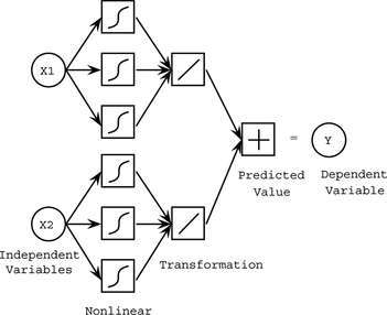
Sarle (1994) proposed the following neural network for a generalized additive model (Figure 1).

FIGURE 1 Generalized additive network.

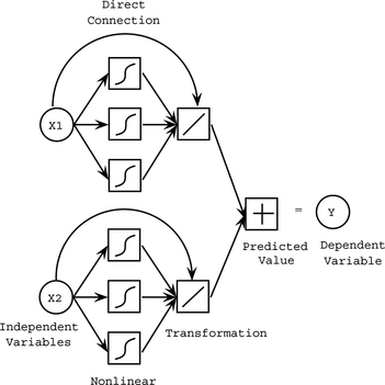
Because MLPs are universal approximators that can model any continuous function (Ripley 1996), Potts (1999) suggested an MLP that has a single layer with h hidden neurons for each input. Furthermore, the basic architecture of Sarle was enhanced with an additional parameter for a direct connection (skip layer) so that the linear model is a special case. The enhanced architecture has the form

The updated generalized additive neural network is given in Figure 2.

FIGURE 2 Enhanced generalized additive network.

The effect of the individual inputs, adjusted for the effect of the other inputs, can be investigated by considering partial residuals (Ezekiel 1924; Larsen and McCleary 1972; Berk and Booth 1995). The jth partial residual is the deviation between the actual values and that portion of the fitted model that does not involve x _j :

Potts (1999) also presented an interactive construction algorithm using partial residual plots to optimize the number of neurons in each variable's hidden layer. These plots of the fitted univariate functions, , overlaid on the partial residuals versus the corresponding jth input, are utilized to assist the model selection process for GANNs. The following recipe was proposed to simplify optimization and model selection:

1.	Construct a GANN with one neuron and a skip layer for each input (inputs are assumed to be standardized):
2.	This gives four parameters (degrees of freedom, df) for each input. Binary inputs (dummy variables) only have a direct connection (1 df).
3.	Fit a generalized linear model to give initial estimates of β0 and w 0j .
4.	Initialize the remaining three parameters in each hidden layer as random values from a normal distribution with mean zero and variance equal to 0.1.
5.	Fit the full GANN model.
6.	Examine each of the fitted univariate functions overlaid on their partial residuals.
7.	Prune the hidden layers with apparently linear effects and add neurons to hidden layers where the nonlinear trend appears to be underfitted. If this step is repeated, the final estimates from previous fits can be used as starting values.

Although the proposed recipe is adequate for solving a large class of problems, it has some drawbacks:

	The method is subjective because it relies on human judgment to identify trends in partial residual plots.
	Executing the recipe can be very time consuming when the problem contains a large number of variables.

A case can therefore be made for automating the proposed recipe. This is described in the Automation section.

Augmented Partial Residual Plots

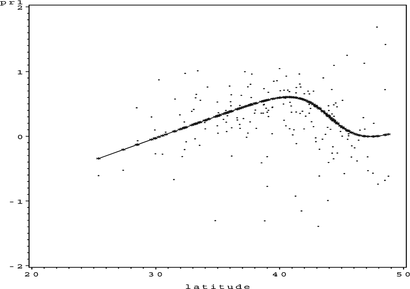
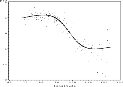
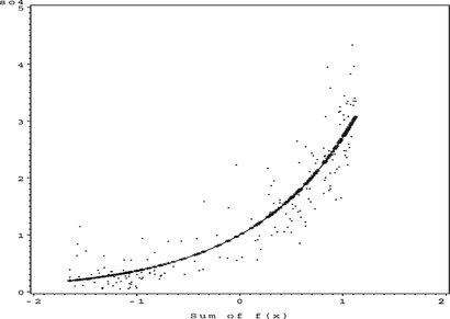
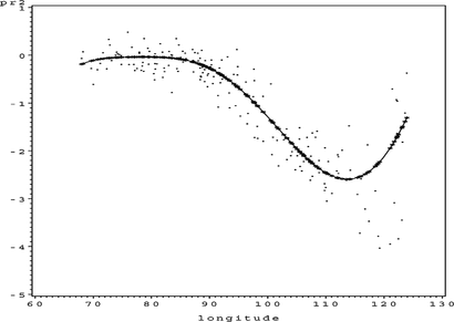
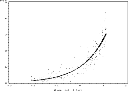
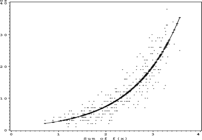
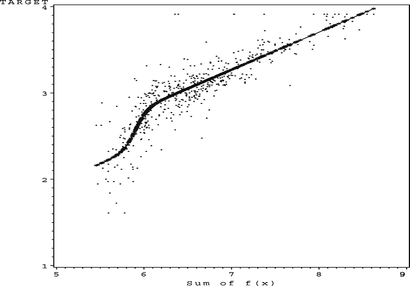
In this article, the partial residual plots are augmented with extra information showing the corresponding univariate function value for each data point. This is important because the fitted cubic spline through the function values could be misleading. Another useful way to present the results is to plot overlaid on E(y) (called the sum of f(x) plot in the rest of the article). This shows the effect of the output activation function (the inverse of the link function). Examples of these plots can be seen in the S O ₄ example below.

S O ₄ Example

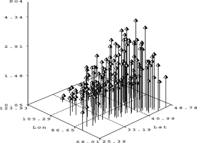
Consider the S O ₄ data set from Xiang (2001) with 179 observations for variables Latitude and Longitude. They represent the latitude and longitude, respectively, of different locations in the United States. The response variable S O ₄ represents the amount of sulfate deposits measured at the corresponding locations. This example was chosen not for its complexity or number of observations but because the results can be graphically displayed and the differences between the various algorithms can easily be highlighted using surface plots. This example will be used as a running example in the rest of the article. Figure 3 contains a stem plot of the data.

FIGURE 3 S O ₄ stem plot of deposits.

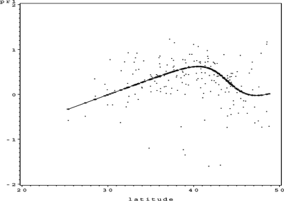
Executing steps 1 to 4 of Potts’ recipe produces the results presented in Figures 4-7.

FIGURE 4 S O ₄ partial residual plot for Latitude.

FIGURE 5 S O ₄ partial residual plot for Longitude.

FIGURE 6 S O ₄ sum of f(x).

FIGURE 7 S O ₄ surface plot.

The model has nine parameters, an average squared error (ASE) of 0.180485, and a Schwarz Bayesian criterion (SBC) value of −259.78.

This looks like a reasonable additive model, but inspection of the partial residual plots leaves some doubt over the fitted univariate function for Longitude: should the function be more complex? Applying steps 5 and 6 of the algorithm and increasing the complexity of the univariate function for Longitude produces the results shown in Figures 8-11.

FIGURE 8 S O ₄ partial residual plot for Latitude.

FIGURE 9 S O ₄ partial residual plot for Longitude.

FIGURE 10 S O ₄ sum of f(x).

FIGURE 11 S O ₄ surface plot.

This model has 12 parameters, an ASE of 0.18027, and an SBC value of −244.43160. Although the model's ASE is slightly lower than that of the previous model, this has been achieved with a large increase in the number of parameters, namely three. Some other statistic now has to be used to decide upon the best model. The first model's SBC value is substantially better (more negative) than that of the second model, so the authors would chose the first model as the final model.

Even for this almost trivial problem, it is not obvious from the partial residual plots which model to select as the final model.

If other statistics, like SBC, have to be used to facilitate the final decision, the question now arises as to why these statistical measures are not incorporated into the algorithm from the start. This provides the motivation for automating the algorithm that is described in the next section.

AUTOMATION

Automation of the recipe given in the GANN Architecture section is not a trivial task, but it was successfully done by Du Toit (2006). In this section an automated algorithm is presented that will find the optimal generalized additive neural network architecture given enough time.

Automated Construction of GANNs

Let each GANN architecture be represented by a string over a finite alphabet. The alphabet consists of 10 symbols (digits) that are given in Table 1.

TABLE 1 GANN Architecture Symbols

Symbol	Description
0	No MLP (input removed from the model)
1	MLP with a skip layer
2	MLP with no skip layer and 1 hidden node
3	MLP with a skip layer and 1 hidden node
4	MLP with no skip layer and 2 hidden nodes
5	MLP with a skip layer and 2 hidden nodes
6	MLP with no skip layer and 3 hidden nodes
7	MLP with a skip layer and 3 hidden nodes
8	MLP with no skip layer and 4 hidden nodes
9	MLP with a skip layer and 4 hidden nodes

The restriction to a finite alphabet is not strictly needed, because the model selection criterion or cross-validation will prevent neural networks that are too complex from being exploited. Also, in the interactive algorithm, a skip layer is always included. This restriction is relaxed in the automated algorithm.

A well-formed string consists of a finite number of digits from the alphabet. For example, the string 102003313 represents a GANN architecture with nine variables where variables 2, 4, and 5 are deleted; variables 1 and 8 are each represented by an MLP with only a skip layer; variable 3 is represented by an MLP with no skip layer and one node in a hidden layer; and variables 6, 7, and 9 are each represented by an MLP with a skip layer and one node in the hidden layer. Each digit in the string represents an architecture for a specific variable (called a subarchitecture). Every well-formed string specifies a model in the GANN model space.

To achieve specific aims such as the reduction in the size of the search space or limiting the complexity of the univariate functions, further restrictions might be placed on the given alphabet (only certain digits allowed).

The problem can now be formulated as a state space search problem:

	States: Any valid GANN architecture corresponding to a well-formed string as described above.
	Initial state: The GANN architecture representing the linear model.
	Successor function: Any GANN architecture with one digit mutated.
	Goal test: No goal test: the best state is reported when the time runs out or the search space is exhausted.
	Path cost: The path cost is unimportant as we are only interested in the best state, not how it was reached.

The automated algorithm is presented as a variation of best-first search (Luger 2005). Note that because we are only interested in the best node and not in the solution path, there is no need to keep track of how the current state was reached. However, because a tree structure is intrinsic to the operation of the automated algorithm, the path from the initial state to the goal is highlighted in most of the examples in the rest of the article. This is just as an aid to facilitate a better understanding of the developed strategy.

The last issue that needs to be resolved before the algorithm is described is the heuristic function that will be used. This is one of the most important issues and the success or failure of the above algorithm depends to a large extent on specifying an appropriate heuristic measure. In Lee (1999), the SBC was proposed as a suitable measure for evaluating MLPs. Du Toit (2006) showed that SBC is also a suitable measure for GANNs. Using SBC as the heuristic function has the added benefit that it is well understood and that it has a sound statistical basis (unlike some ad hoc heuristic function that were proposed in the literature to select the best neural network architecture).

Several forms of the Schwarz information criterion (SIC or SBC) have been proposed in the literature. The generic SBC is defined as follows (Burnham and Anderson 2002):

where denotes the natural logarithm of the likelihood function of the parameter vector θ, given the data y, K the number of estimable parameters in the approximating model, and n the size of the data set. In the special case of the Gaussian error model, the SBC can be expressed as

where

ε _i are the estimated residuals for a particular candidate model, and K is the total number of estimated regression parameters including the intercept and σ². Models are evaluated on the validation data set when a validation data set is present, which allows the algorithm to perform cross-validation.

A high-level description of the automated GANN construction algorithm is given as Function autogann_v1 below. A few comments on the differences between Potts's (1999) algorithm and the automated algorithm is in order.

First, during the expansion step (Step 6 of the interactive construction algorithm), any number of neurons may be added or deleted from the hidden layer of each variable. This is a very general step that needs to be structured to make automation possible. This issue is resolved by restricting the successor function to subarchitectures in the row above or the row below the current subarchitecture (see Table 1 for an ordering of architectures from simple to complex). This implies that the successor function can only make slight changes to the underlying neural network sub-architectures. The restriction makes the number of steps that needs to be considered during each iteration of the automated algorithm manageable (maximum twice the number of variables).

begin

start := linear_model;

open := [start];

closed := [];

 while open ≠ [] and the search time has not elapsed do

 remove the leftmost state from open, call it X;

 begin

 generate children of X;

 for each child of X do

 if the child is not on open or closed then

 assign the child a heuristic value;

 add the child to open;

 end

 end

 end

 add X to closed;

 re-order states on open by heuristic merit (best leftmost);

 end

 return best state (using heuristic merit) from open and closed;

end

Function autogann_v1

Second, the search for the best GANN model and associated architecture is now organized in the form of a search tree. Offspring or children of a GANN model are generated by the successor function. Nodes are ordered according to some model selection criterion (such as the SBC or cross-validation error), and the node with the best model selection criterion value is expanded next. The search continues until the search space is exhausted or a predetermined time limit has been exceeded.

Third, duplicate states are also not allowed in the search tree and because there are upper and lower limits to the complexity of the underlying GANN architecture (see Table 1), the branching factor decreases as the search tree is expanded. In effect, a greedy best-first search strategy is executed with the ordering based on objective model selection criteria or cross-validation error.

Fourth, the interactive construction algorithm starts from a nonlinear model to aid interpretation of the partial residual plots (it is easier to interpret slightly nonlinear trends than linear trends in the partial residual plots(Berk and Booth 1995). Because the inspection of partial residual plots no longer drives the operation of the algorithm, any starting point may be chosen. The linear model is used as a starting point for the automated construction algorithm because variables can then be immediately deleted from the model through one application of the successor function. Irrelevant variables are therefore quickly removed, which simplifies the GANN architecture and speeds up later training.

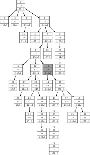
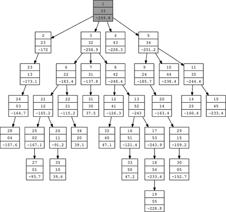
Application of Function autogann_v1 to the S O ₄ data set produces the result in Figure 12 with the subarchitectures restricted to 0, 1, 2, 3, 4, and 5.

FIGURE 12 S O ₄ search tree generated by autogann_v1.

Note the following:

	Each node shows the order of generation, the GANN architecture, and SBC value.
	The best node generated was the 13th node (colored grey).
	The path from the root node (node 1) to the best node is highlighted with thicker lines.
	The best model has a heuristic value of: SBC = −259.8.
	The best GANN architecture contains an MLP with a skip layer and one hidden node for each variable, represented by the string 33.
	The model space contains 6 ∗ 6 = 36 models, but because the trivial model 00 is not generated, there is a maximum of 35 models in the tree (this is a restriction of proc neural in Enterprise Miner™ (SAS Institute Inc. 2007) in which the algorithm is implemented).

Although the above algorithm is sound, it becomes impractical for larger problems because many levels in the search tree are needed to generate the best GANN architecture. The tree also becomes very large and unwieldy. This is partly the result of restricting the successor function to one change in the architecture. The removal of this restriction is described next.

Multistep Expansion

In the algorithm presented so far, only one change is allowed to the GANN architecture in each child node (see Figure 12). This restriction forces one iteration of the algorithm for each change in architecture. For a large number of variables, the number of applications of the successor function needed to arrive at the optimal GANN architecture becomes unrealistically large. The relaxation of this restriction is described next.

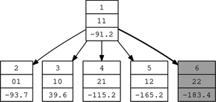
When two or more child nodes (with a common parent node) have model selection criterion values better than that of the parent node, it could be prudent to allow multiple changes. This can be done as follows. Identify all the child nodes with model selection criterion values better than that of the parent node. In the example of Figure 13, this corresponds to nodes 2, 4, and 5. Create a new (sibling) child node (node 6) from the common parent node inheriting all changes in the identified children. When two child nodes have better model selection criterion values than the parent node for the same change in subarchitecture (nodes 2 and 4), use the change in the best one (node 4). Because all of the changes have been identified as being worthwhile independent of each other, there exits a good probability that all the changes applied collectively will also be worthwhile. Multiple changes are therefore allowed during an iteration of the algorithm.

FIGURE 13 S O ₄ multistep expansion.

This heuristic has a direct equivalent in the interactive algorithm. During each iteration of the interactive algorithm, multiple changes would have been made to the GANN architecture based on inspection of partial residual plots. The heuristic therefore models one iteration of the interactive algorithm. Because convergence (a model exhibiting satisfactory fits in all partial residual plots) of the interactive algorithm is usually attained within a few iterations, the automated algorithm should exhibit a similar trend.

Improved Multistep Expansion

In Step 6 of the interactive algorithm, no restrictions are placed on the number of hidden nodes that may be added to or removed from a hidden layer after inspection of the associated partial residual plot. To arrive at an automated algorithm, the successor function was restricted to slightly more complex or slightly less complex subarchitectures for efficiency reasons.

This restriction can be removed as follows. For each generated child node with a model selection criterion value better than that of the parent node, do another application of the successor function from the generated child node (on the same variable) and examine the resulting model selection criterion value of the newly generated node. If the model selection criterion value improved, repeat the process of generating additional child nodes until the model selection criterion value of the last generated node becomes worse. Consider the best node generated during this recursive process as the result of the application of the successor function. This strategy allows moves in the subarchitectures to nonadjacent rows of Table 1. Figure 14 contains an example of such a step from the S O ₄ data set. The best node is colored grey.

FIGURE 14 S O ₄ improved multistep expansion.

Although the strategy is sound and may decrease the number of iterations necessary in the automated algorithm, it has a major drawback in that intelligent search is partly replaced by enumeration, which is counterproductive. It is also very unlikely that even the experienced modeler will be able to make such dramatic changes based on the inspection of partial residual plots (the complexity vs. degrees of freedom tradeoff is not easy to judge).

An approximation to the above strategy that can be efficiently computed is now presented. Because the search in the automated strategy is started from the linear model, only an increase in the complexity or number of hidden nodes will be considered. Instead of reevaluating each additional child node (which involves the training of a neural network), just adjust the first child node's (node 2 in Figure 14) model selection criterion value with the extra degrees of freedom (K) applicable to each additional child node (nodes 3 and 4 in Figure 14), keeping the maximum likelihood estimate constant (this will work for SBC but not with cross-validation). This gives an approximation to the child nodes’ model selection criterion values and can be computed directly without any optimization. The model selection criterion values will now become worse during each evaluation of each additional child node and at some stage will be worse than that of the parent node when this process started. This gives an approximation to the maximum possible moves in sub-architecture.

In the implementation used to compute the results given in this article, the maximum move is restricted to two rows of Table 1 when the approximation indicates that a move of three or more steps is possible. In effect, a test is done to estimate the scope of the model improvement. If the scope for improvement is substantial (the degrees of freedom of the child node can be increased without obtaining a model selection criterion value worse than that of the parent node), a possibility exists that a more complex subarchitecture will also give a better model.

Intelligent Start

In the automated algorithm, the search is started from the linear model. In this section, a preprocessing step is described that adjusts some of the linear model's subarchitectures to more “promising” subarchitectures. The start architecture has a dramatic influence on the path that is followed to reach the expected results as well as the time needed to compute the result. An “intelligent guess” of an appropriate final model architecture could therefore dramatically decrease the number of steps needed to arrive at the final model. A preprocessing step that is based on an analysis of the results of a stepwise regression is described next.

After a generalized additive model with one neuron and a skip layer for each input has been constructed and the neural network trained with the default optimization algorithm, the GANN is reformulated as a regression problem. In the regression formulation, seperate variables are created for each skip layer and each hidden layer (with all its parameters). A stepwise regression is then performed on the reformulated problem and the results are interpreted as a GANN. Variables not selected by stepwise regression indicate which skip layers and hidden layers can be removed from the GANN. The resulting GANN is used as the new intelligent start architecture. Function intelligent_guess is given below.

An updated autogann algorithm is now presented that will find the optimal architecture for the revised generalized additive network in a reasonable amount of time. The philosophy behind the updated algorithm is also different from that presented by Du Toit (2006): instead of starting from the linear model and searching for the optimal GANN architecture, the updated algorithm makes an intelligent guess of the best architecture and then attempts to refine the guess to arrive at the best architecture.

begin

 construct a GANN with one neuron and a skip layer for each input V _j , call it Guess

 f _j (x _ij ) = w _0j x _ji  + w _1j tanh(w _01j  + w _ji );

 fit the GANN model;

 for each input variable V _j in the GANN model do

V _j _skip := w _0j x _ji ;

V _j _hidden := w _1j tanh(w _01j  + w _ji );

 end

 fit a stepwise regression model using the new variables V _j _skip and V _j _hidden;

 for each input variable V _j in the GANN only do

 case only V _j _skip is included in the selected regression model

 delete the one neuron for variable V _j from Guess f _j (x _ji ) = w _0j x _ji ;

 end

 case only V _j _hidden in included in the selected regression model

 delete the skip layer for variable V _j from Guess f _j (x _ji ) = w _1j tanh(w _01j  + w _ji );

 end

 case neither V _j _skip nor V _j _hidden are included in the selected regression model

 delete variable V _j from Guess;

 end

end

return Guess;

end

Function intelligent_guess

The multistep expansion operation and the intelligent guess of the best architecture have a dramatic effect on the efficiency of the algorithm. If the intelligent guess of the best architecture is correct, no search is required. The algorithm is given as Function autogann_v2 below.

Returning to our running example, a 10-s run of the algorithm using 0, 1, 2, 3, 4, and 5 from Table 1 as possible subarchitectures for each variable produces the results given in Figure 15.

FIGURE 15 S O ₄ search tree generated by autogann_v2.

The intelligent guess produced the optimal GANN architecture, so no search was therefore needed to obtain the optimal result (the gray-colored node is the best node). The problem of which model to select as the best model experienced with the recipe of Potts (1999) has been effectively resolved with the automated algorithm.

LINK FUNCTION

In the proposed architecture, the link function defines the output activation function (the inverse of the link function). Examples of link functions are the logit function, the log function, and the identity function.

In many cases the link function is unknown. A guess must therefore be made of an appropriate link function and one selected from a list of available functions. But, because the link function is also a univariate function, it can be approximated with a neural network in a similar manner as the univariate functions of the independent variables.

begin

 start := intelligent_guess; open := [start]; closed := [];

 while open ≠ [] and the search time has not elapsed do

 remove the leftmost state from open, call it X;

 begin

 crossover := []; threshold := heuristic value of X;

 minimum := heuristic value of X; generate children of X;

 for each child of X do

 if the child is not on open or closed then

 assign the child a heuristic value; add the child to open;

 if heuristic value of child < threshold then

 add child to crossover; minimum := heuristic value of child;

 end

 end

 end

 if crossover contains at least two states then

 construct a super child from crossover, call it S;

 if S is not on open or closed then

 assign S a heuristic value;

 if heuristic value of S < minimum then

 add S to open;

 end

 end

 end

end

add X to closed;

re-order states on open by heuristic merit (best leftmost);

end

return best state (using heuristic merit) from open and closed;

end

Function autogann_v2

The enhanced architecture of Potts (1999) is now further enhanced (generalized) with additional nodes implementing the output activation function. The new architecture is described in more detail in the following section.

GENERALIZED GANN ARCHITECTURE

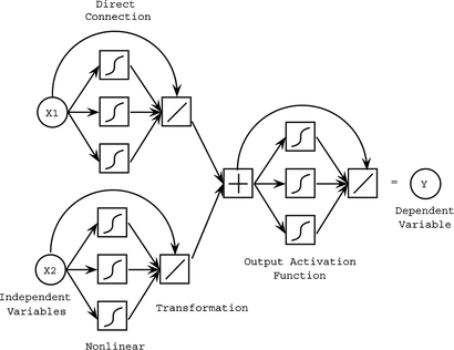
The architecture of Potts (1999) is generalized with an additional hidden and output layer that will compute the output activation function. Figure 16 contains the generalized architecture.

FIGURE 16 Link-enhanced generalized additive network.

Note that the previous architecture of Potts (1999) is a special case of this architecture: the part of the network computing the output activation function only has a direct connection with weight frozen to 1 and the final transformation implements the known output activation function. The new enhanced architecture has the following benefits:

1.	The link function does not need to be specified a priori.
2.	Any link function can be approximated with the architecture.

In the case of a binary classification problem, it would be a good idea to change the linear output activation function to the logistic function to constrain the probabilities to [0, 1].

The automated algorithm can be applied to the revised architecture in an elegant way. Add an extra symbol (digit) to the well-formed string representing the GANN architecture. This extra symbol represents the output activation function. For reasons of clarity, the digit is appended to the back of the well-formed string separated by a dash (–). This is only syntactic and has no bearing on the algorithm. The autogann algorithm can now be applied without modification to the new architecture or string. This result shows the elegance of the notation and the generality of the algorithm developed above.

Table 2 shows the format of the link and output activation functions for sub-architecture symbols 0, 1, and 2, where n = β₀ + f ₁(x ₁) + f ₂(x ₂) + … + f _k (x _k ), and w _i , w _j , and w _k are estimable parameters of the output activation function.

TABLE 2 Format of Link and Activation Functions

Symbol		E(y)	Target range
0	ln[E(y)]	e ^n	(0, ∞)
0			[0, 1]
0			[−1, 1]
0	n	n	(−∞, ∞)
1		w i n	(−∞, ∞)
2			(−∞, ∞)

When an output activation function represented by the symbol 0 is selected, the range of the target values determines its functional form. In general, link functions for subarchitecture symbols 3 to 9 are undefined, because the corresponding output activation functions are not one-to-one. Therefore, partial residual plots can only be produced for output activation functions with subarchitecture symbols 0, 1 or 2. In the latter case the partial residuals are undefined when

a.	or
b.	w i  − E(y) = 0 or
c.	w k  = 0.

The authors De Waal and du Toit, considered two algorithms to compute the undefined partial residuals. Newton's method (Deuflhard 2004) did not converge on the S O ₄ data set. The bisection method (Conte and De Boor 1965; Corliss 1977) successfully computed the unknown partial residuals.

Bisection Method

Recall from the GANN Architecture section that

where is unknown. To determine the latter, let g ₀(x) be the continuous output activation function for subarchitecture symbol 2 on the closed interval [a, b], where and x ∈ [a, b]. If

then g ₀(x) − E(y _i ) has one root on (a, b). The bisection method generates a sequence of intervals on which the root is known to lie and is guaranteed to converge to the root, .

S O ₄ Example

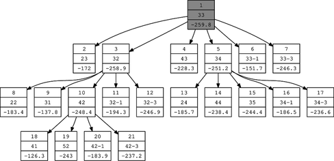
A 5-s run of Function autogann_v2 with an intelligent guess of the start architecture, subarchitectures 0, 1, 2, 3, 4, and 5 available for the univariate functions of the inputs and subarchitectures 0, 1, 2, and 3 available for the output activation function, produces the following results. During the 5 seconds 21 models were generated and arranged in the following search tree given in Figure 17. The model space consists of 6 ∗ 6 ∗ 4 = 144 models (although only 140 models are generated by the algorithm due to the restrictions of the underlying neural network procedure discussed earlier).

FIGURE 17 S O ₄ search tree generated by autogann_v2.

Note that the intelligent guess again produced 33 as start architecture and that this is still the best model when considering SBC as model selection criterion. However, the best model with a link function other than the log link function is the model represented by the string 32-3 (node 12 at depth 2 of the search tree; see Figure 17). This model has 12 parameters, an ASE of 0.177827, and an SBC value of −246.9 (compared to 9 parameters, an ASE of 0.180485, and a SBC value of −259.8 for the best mode indicated by the string 33).

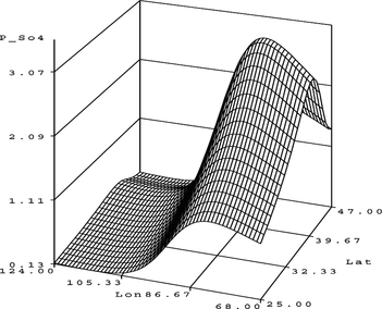
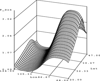
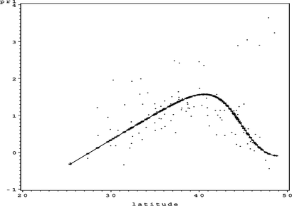
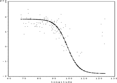
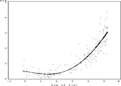
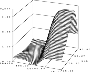
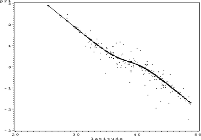
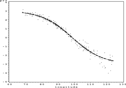
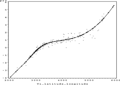
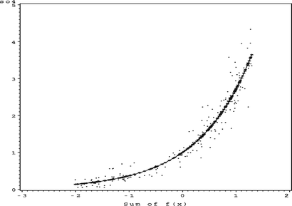
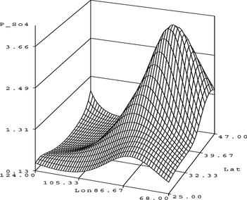
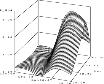
The following partial residual plots (Figures 18 and 19) for the input variables, sum of f(x) plot, (Figure 20) and surface plot (Figure 21) for the output activation function are generated.

FIGURE 18 S O ₄ partial residual plot for Latitude.

FIGURE 19 S O ₄ partial residual plot for Longitude.

FIGURE 20 S O ₄ sum of f(x).

FIGURE 21 S O ₄ surface plot.

It is clear from Figure 20 that the link function is not monotonic any more. This creates several difficulties when generating partial residual plots as discussed in the Generalized GANN Architecture section. Some of the partial residuals shown in the partial residual plots (Figures 18 and 19) could therefore be wrong and the reader should be aware of this fact. However, the authors still feel that the partial residual plots are useful for interpreting trends and they are therefore included in the visual diagnostics. In the case that the link function is complex (but monotonic), the partial residual plots are still correct, although the partial residuals are now generated using the bisection method.

Note further that the log link function exploited in the best model (according to SBC) is not the optimal link function for this particular problem (see Figure 20). A slight variation of the log link function may produce even better results. But, for this example, the more accurate link function is obtained at the expense of an extra 4 degrees of freedom, which does not lead to a model with a better SBC value.

The astute reader may now ask whether it is possible to identify and compute the optimal transformations for the univariate functions (including the link function). This topic is further investigated in the Comparison section when the approach presented in this article is compared to alternating conditional expectations (ACE), which identifies optimal transformations for multiple regression problems.

Note that for large Latitude and Longitude values the surface gravitates upward and the experienced modeler may argue that an even better model may be obtained by including interaction terms in the model. This line of thought is further developed in the Comparison section when GANNs are compared to MLPs.

This section is concluded with a slightly more complex example.

Ozone Example

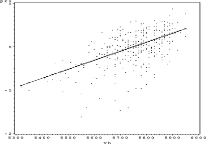
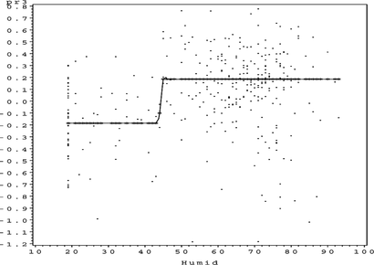
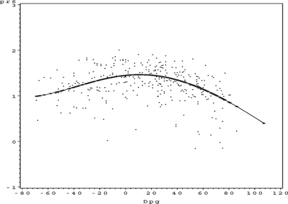
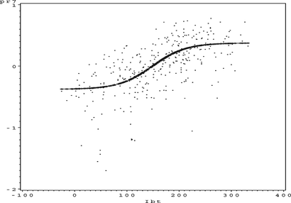
The ozone data set of Breiman Friedman(1985) has 330 observations of the target variable, ground-level ozone (as a pollutant), and nine explanatory variables. Eight of the inputs are broadly meteorological by nature and the ninth is the day of year. The inputs are: VH, the altitude (m) at which the pressure is 500 millibars; WIND is the wind speed (mph) at the Los Angeles International Airport (LAX); HUMID is the humidity (%) at LAX; TEMP is the temperature (°F) at Sandburg Air Force Base; IBH is the temperature inversion base height (feet); DPG is the pressure gradient (mmHg) from LAX to Daggert; IBT is the inversion base temperature (°F) at LAX; VIS is the visibility (miles) at LAX; and DOY is the day of year.

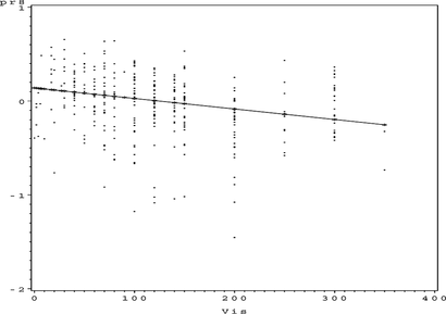
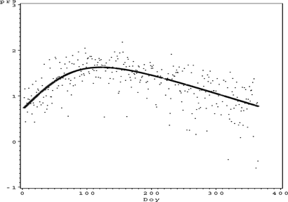
The best model found when the algorithm autogann_v2 is executed for 45 s using 0, 1, 2, 3, 4, and 5 from Table 1 as possible subarchitectures for the inputs and 0, 1, 2, and 3 as possible architectures for the link functions is 102003213. This model has 17 parameters, an ASE of 11.27621, and an SBC value of 898.07387. Figures 22-28 show the corresponding partial residual plots and output activation function.

FIGURE 22 Ozone partial residual plot for VH.

FIGURE 23 Ozone partial residual plot for HUMID.

FIGURE 24 Ozone partial residual plot for DPG.

FIGURE 25 Ozone partial residual plot for IBT.

FIGURE 26 Ozone partial residual plot for VIS.

FIGURE 27 Ozone partial residual plot for DOY.

FIGURE 28 Ozone sum of f(x).

A number of people analyzed this data set in the nonparametric regression literature(Lee 1999). Breiman and Friedman (1985) used this data set in their paper on ACE. They utilized the estimated multiple correlation coefficient, R ², as a goodness-of-fit measure and fitted the model using a subset of only four variables (TEMP, IBH, DPG, and VIS) that were chosen by a stepwise algorithm.Hastie and Tibshirani(1986) fitted a generalized additive model to the data.

Friedman and Silverman (1989) used TURBO to fit the data. Hawkins (1989) discussed the previous paper and fitted the data with linear regression after using Box-Tidwell-style transformations on the variables. Lee (1999) utilized an MLP neural network model with three nodes in the hidden layer and five independent variables. Table 3 indicates that all of the above methods have similar goodness-of-fit to the data. All of the methods do find a reasonable fit, but none is substantially better than the others.

TABLE 3 Comparison of Competing Methods

Method	R ^2
ACE, four variables	0.78
GAM	0.80
TURBO	0.80
Box-Tidwell	0.82
Neural network	0.79
autogann_v2	0.82

COMPARISON

Multilayer Perceptrons

One of the disadvantages of additive models (in their simplest form) is their inability to model interactions. One possible remedy is to add explicit interaction terms/variables to the set of independent variables. The interaction variables are then treated as normal variables and the model estimated in the usual manner. The result of adding explicit interaction variables (only Latitude ∗ Longitude in this case) to the S O ₄ data set and a 45-s run of Function autogann_v2 described in this article is given below. In the allotted time, 109 models were generated. Figures 29, 30, and 31 contain the partial residual plots and Figure 32 shows the scatterplot for the output activation function.

FIGURE 29 S O ₄ partial residual plot for Latitude.

FIGURE 30 S O ₄ partial residual plot for Longitude.

FIGURE 31 S O ₄ partial residual plot for Latitude ∗ Longitude.

FIGURE 32 S O ₄ sum of f(x).

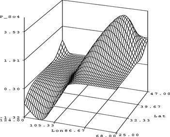
The model is represented by the string 325 and has 15 parameters, an ASE of 0.085327, and a SBC value of −362.75. It is substantially more accurate than any of the models obtained earlier. The surface plot is given in Figure 33.

FIGURE 33 S O ₄ surface plot.

However, to judge the accuracy of this model it is compared to a neural network (MLP) with a similar number of parameters. The neural network is therefore restricted to an MLP with one hidden layer containing four hidden nodes. The surface plot of the model obtained by the neural network is given in Figure 34.

FIGURE 34 S O ₄ surface plot.

The MLP has 17 parameters, an ASE of 0.086678 and an SBC value of −349.57. According to the generated SBC values, the GANN produces a better model than the MLP for similar numbers of parameters. This surprising result is explained next.

In the GANN the interactions have now been made explicit and the contribution of the interaction terms can be analyzed using partial residual plots. This gives added insight into the model that is not possible with an MLP, because the interactions in the MLP are intertwined with contributions of the inputs. The GANN model is also more parsimonious because it allows finer control over the number of parameters in the model than is possible with an MLP.

In an MLP with one input layer, one hidden layer, and one output layer, all of the nodes in the input layer are connected to all of the nodes in the hidden layer. For example, if the problem at hand has five inputs, the hidden layer 10 nodes, and the output layer 1 node, the number of parameters increases or decreases in multiples of seven when a node is added or removed from the hidden layer (five inputs connected to the node, a bias, and a connection to the output layer). The optimal model may be a model with a number of parameters different from that generated by the MLP described above.

Furthermore, according to the rule of thumb stating that at least 10 records are needed to accurately estimate a parameter (Zhang, Patuwo, and Hu 1998), this gives a maximum of 18 parameters for the S O ₄ problem (the data set has 179 records). The number of parameters in the GANN model is well within this threshold, but the number of parameters for the MLP needs to be increased to arrive at a decent model taking it over this threshold.

Alternating Conditional Expectations

The ACE algorithm was developed by Breiman and Friedman (1985) as a tool to estimate optimal transformations for multiple regression problems. Their goal was to find those transformations that produce the best-fitting additive model. The goal of Function autogann_v2 is to find the best generalized additive model based on an objective model selection criterion (e.g., SBC). This will not necessarily produce the best fitting additive model and optimal transformations, but the model will be parsimonious and will generalize well on unseen data.

Although the aims of both methods are fairly similar, the methods employed to obtain the required results are very different. The approach of Breiman and Friedman (1985) is based on a simple iterative algorithm using only bivariate conditional expectations, which converges to an optimal solution. When the conditional expectations are estimated from a finite data set, the algorithm results in estimates of the optimal transformations. The method depends on the estimation of various smoothers for its success.

The full ACE algorithm for minimizing squared error is presented as Function ace below.

The transformations θ, φ₁, …, φ _p computed by the ACE algorithm correspond closely to the univariate functions computed by the autogann_v2 algorithm.

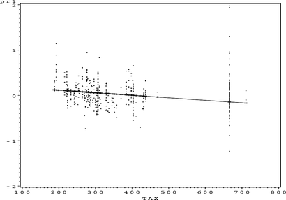
Recently, Campher (2008) did a comprehensive comparison between the system described in this article, ACE, and decision trees using various simulated and other data sets. In six of the seven examples studied, GANNs outperformed ACE. One of the original examples studied by Breiman and Friedman (1985) is the Boston housing marketing data (Harrison and Rubinfeld 1978), initially investigated to determine how various factors might affect the housing values in the Boston Standard Statistical Metropolitan Area in 1970. The data set has 506 observations of the target variable, median value of owner-occupied homes (MEDV), and 12 explanatory variables. In one of Breiman and Friedman's (1985) experiments only four inputs are used. The inputs were RM, average number of rooms in owner units; LSTAT, proportion of population that is lower status; PTRAT, pupil–teacher ratio by town school district; and TAX, full property tax rate. Harrison and Rubinfeld's (1978) analysis suggested the following transformations: RM is replaced by R M ², LSTAT is replaced by log(LSTAT), and MEDV is replaced by log(MEDV).

begin

 set θ(Y) = Y/||Y|| and φ₁(X ₁),…, φ _p (X _p ) = 0;

 while e ₂(θ, φ₁,…, φ _p ) fails to decrease do

 while e ₂(θ, φ₁,…, φ _p ) fails to decrease do

 for k = 1 to p do

 θ _k,1(X _k ) = E[θ(Y) − ∑ _i≠k φ _i (X _i )|X _k ];

 replace φ _k (X _k ) with φ _k,1(X _k );

 end

 end

 θ₁(Y) = E[∑φ _i (X _i )|Y]/||E[∑φ _i (X _i )|Y]||;

 replace θ(Y) with θ₁(Y);

 end

 return θ, φ₁,…, φ _p ;

end

Function ace

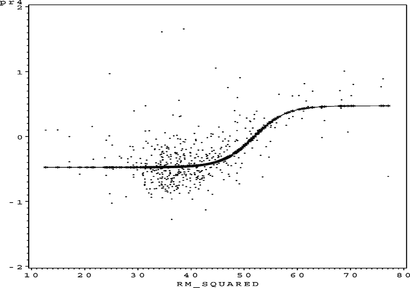
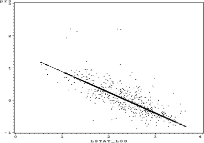
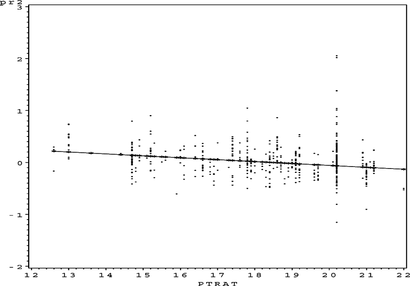
Figures 35-38 contain the partial residual plots computed by Function autogann_v2 for the simplified problem described above after a 90-s run of autogann_v2.

FIGURE 35 S O ₄ partial residual plot for R m ².

FIGURE 36 S O ₄ partial residual plot for log(Lstat).

FIGURE 37 S O ₄ partial residual plot for PTRAT.

FIGURE 38 S O ₄ partial residual plot TAX.

The best model is represented by the string 1112-3. It has 11 parameters, an ASE of 0.035932 and an SBC of −1,614.52. Note further that all of the refinements to the original approach of Potts (1999) presented in this article were needed to compute this result. The link function was computed by a separate neural network, the partial residuals were computed with the bisection method, and the optimal model architecture was identified automatically without any user intervention.

The computed univariate functions (indicated by the fitted splines) are very similar to that computed by the smoothers in Breinman and Friedman (1985). Note, however, that in this article the computed univariate functions are given as part of the partial residual plots and not as stand-alone functions. This provides more visual information on the appropriateness of the transformations. The sum of f(x) plot in Figure 39 shows the effect of the log transformation on the target variable MEDV. Breiman and Friedman (1985) hinted that the original log transformation done on the target variable MEDV by Harrison and Rubinfeld (1978) was too severe. Figure 39 contains the new transformation (link function) for log(MEDV). This link function is attempting to reverse/negate the effects of the log transformation and confirms the comment by Breiman and Friedman (1985).

FIGURE 39 S O ₄ sum of f(x).

Stability of the ACE algorithm is highly dependent on the type of smoother used(Breiman and Friedman 1985). Even when the supersmoother is used, it does not always produce stable results, especially near the boundaries of the problem input space. This is not the case with the GANN algorithm. Table 4 contains a high-level comparison between ACE and Function autogann_v2.

TABLE 4 GANN vs. ACE

	ACE	autogann_v2
Basis function	Smoother	Sigmoidal function
Variable order	Important	Irrelevant
Specifying of of user parameters	Not trivial	Trivial
Generalization	Bass-enhancement	Objective model selection criteria
Optimization	Alternates between input functions and link function	All functions done collectively
Accuracy	Optimal	Optimal given chosen architecture
Speed	Relatively fast	Relatively slow

The speed of the autogann_v2 algorithm can be dramatically increased and autogann_v2 made to even more closely resemble ACE by specifying the GANN architecture a priori. Note further that the supersmoother used in ACE is a variable span-smoother and based on tweeter, mid-range, and woofer smoothers that should reproduce the main parts of the frequency spectrum of f(x) (Friedman 1984).

A five subarchitecture for each variable (a skip layer with two hidden nodes) would allow the GANN to reproduce the tweeter, midrange and woofer smoothers of ACE. It is then left to the optimization algorithm (which minimizes mean squared error) to decide on the complexity of the underlying components (ACE does this in a similar way). If autogann_v2 is specified in this manner, only one run of the Levenberg-Marquardt algorithm is required and it is left to the training algorithm to decide on the importance of links and therefore the complexity of the underlying functions.

Figure 40 contains a surface plot that is generated by the autogann_v2 algorithm with an architecture of 55-3 without any search allowed (a 3 is selected for the link function because it should not be that complex and monotonic if possible). This model has 19 parameters, an ASE of 0.169361, and an SBC value of −219.29. Note that it is still a good model, as can be seen from the smooth surface, and the extra degrees of freedom allowed has not resulted in unforeseen complexity and noise.

FIGURE 40 S O ₄ surface plot.

The question can now be asked what benefits the extra search and refinement of the GANN architecture identified by the search algorithm have over ACE.

There are several benefits to the GANN approach:

1.	The optimal model identified by the autogann_v2 algorithm has a sound statistical basis, it was chosen so that some objective model selection criterion was optimized;
2.	The model was chosen with parsimony in mind (choosing the minimum number of degrees of freedom to obtain a good model). This should assist in generating a model with good generalization capabilities (the bias-variance trade-off has been optimized);
3.	The GANN system produces functions as part of its results. These functions can be used directly to score new data. These functions can also be used to transform the inputs for other modeling techniques.
4.	Relationships between the input variables and the target variable can be investigated with the aid of partial residual plots. Although the method is based on neural networks, it is not a black box.
5.	Automatic variable selection is a result of the algorithm. It is important to remove irrelevant variables and highly correlated variables because it removes noise and simplifies the model, which should result in a better model.
6.	The algorithm is fully automatic and the only user parameter that needs to be specified is the allotted time the algorithm may run. If the user has difficulty in setting the time limit, the maximum time can be specified. The algorithm will then terminate when this time limit has been reached, the model space has been exhausted, or a maximum of 10, 000 models has been generated.

Although the ACE algorithm has been widely praised for its contributions to data analysis(Fowlkes and Kettenring 1985; Pregibon and Vardi 1985), its susceptibility to noise (Esteban-Díez et al. 2006), the need for the user to set parameters has resulted in the scarce practical application of the algorithm. The fully automated algorithm, autogann_v2, presented in this article provides an alternative method of building “optimal” generalized additive models that overcome most of the difficulties associated with the original ACE algorithm. Function autogann_v2 is also implemented in SAS® Enterprise Miner^TM, which should make it usable to a wide community of modelers and analysts.

Support Vector Machines

It is not the aim of this article to provide a complete comparison between the algorithm developed so far and support vector machines. However, due to the increasing popularity of support vector machines, some comments are in order. A similar detailed study between SVMs and GANNs (as was done between ACE and GANNs) is the subject of current research, and results will be published in a separate paper.

Table 5 contains a table highlighting some similarities as well as some differences between the two approaches. This comparison first appeared in r177.

TABLE 5 GANN vs SVM

	SVM	GANN
Nonlinear classifier	Yes	Yes
Maximal separation	Yes	No
Indifferent to kernel choice	No	Yes
Interpretable results	No	Yes

The first two entries in the table are clear: both GANNs and SVMs may be used to build nonlinear classifiers. Furthermore, a classifier implemented as a GANN (with a logit or other link function) does not attempt to achieve maximal separation of the classes.

The third entry can be explained as follows. If one looks at the formulas for SVM using a sigmoid kernel and GANNs with interaction terms added and a hyperbolic tangent activation function, the formulas look remarkably similar. If a problem needs to be solved for which the sigmoid kernel in the SVM is inappropriate, another kernel (for instance, a polynomial kernel) must be chosen. This is unnecessary in the GANN because the new kernel can be approximated with the underlying neural network (each variable has its own MLP that can approximate any continuous function). So in effect the automated GANN algorithm does a search over different “kernels” to compute the nonlinear classifier. Furthermore, let us assume that the optimal classifier for a certain problem needs several kernels. In the GANN it is not an issue, but the SVM choosing some kernel will always be suboptimal.

The fourth entry is also easy to explain: partial residual plots also make GANNs easier to interpret than SVMs. This concludes the brief comparison between the two techniques.

GENETIC ALGORITHM

The diligent reader may also have realized that some aspects of the presented solution closely resemble aspects of a possible genetic algorithm solution and that the encoding of the problem was specifically chosen to resemble the encodings generally found in genetic algorithms(Goldberg 1989). However, the proposed genetic algorithm is to be used for model selection and not to replace back-propagation(Montana and davis 1989).

The required population can be constructed after the number of variables N is known. Individuals in the population are represented by strings consisting of the concatenation of N + 1 symbols from the alphabet given in Table 1. These strings specify the genotype. This represents a weak representation scheme, because the phenotype can only be constructed using the ‘blueprint’ given in Table 1 (Miller, Todd, and Hegde 1989).

The successor function of the automated algorithm closely resembles the mutation operator in genetic algorithms. Mutation in genetic algorithms is usually presented as follows. Each location is subject to a random mutation with a small independent probability. Because of the ordered pruning and growing steps in the interactive algorithm, the mutations are not random (they are restricted to adjacent symbols in Table 1) and have probability one.

The multistep heuristic closely resembles the crossover operator. In uniform crossover, bits (digits in our case) are randomly inherited from the two parent strings. In this case that there may be any number of parents and important bits identified through better model selection criteria, values or validation error values are inherited with probability one.

To arrive at a genetic algorithm for identifying the best GANN model, a fitness function is needed. In this context, such a function can easily be constructed from SBC values or validation error, because these values already specify an ordering of the models.

The only possible complication might be the evaluation of the fitness function. Because the fitness function is based on the fitting of a neural network, it might not be as fast as is usually expected of such a function. These and other issues are investigated in a separate paper.

EXAMPLE

The final example that is considered is a popular example from the UCI Repository, namely, the adult data set(Asuncion and Newman 2007). Recently the data set was also used by pednault (2006) in an article on transform regression.

The prediction task is to determine whether a person makes over 50 K a year. The data set has 48,842 observations of the target variable and 14 explanatory variables. The input variables are age, workclass, fnlwgt, education, education_num, marital_status, occupation, relationship, race, gender, capital_gain, capital_loss, hours_per_week, and native_country.

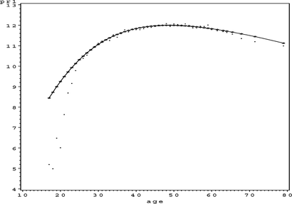
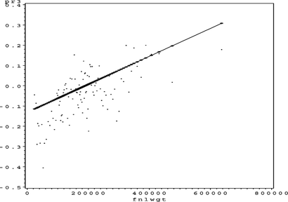
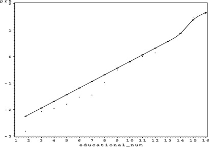
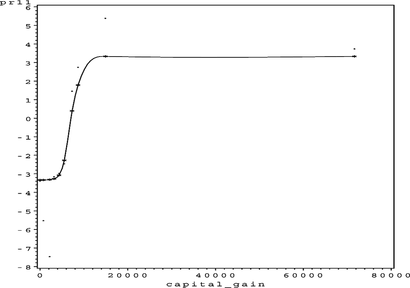
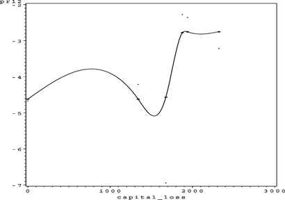
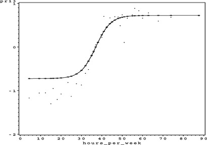
Application of Function autogann_v2 to the data set produces the following results. The best model is represented by the string 31103111012420 (the order of the variables is the same as in the description in the previous paragraph) and has a Gini coefficient is 0.812. The intelligent guess produced the 30103000003330 architecture, of which six digits were carried over to the best architecture. Figures 41-46 contain the generated partial residual plots for the continuous variables.

FIGURE 41 Adult partial residual plot for age.

FIGURE 42 Adult partial residual plot for fnlwgt.

FIGURE 43 Adult partial residual plot for educational_num.

FIGURE 44 Adult partial residual plot for capital_gain.

FIGURE 45 Adult partial residual plot for capital_loss.

FIGURE 46 Adult partial residual plot for hours_per_week.

This model has 57 parameters, an ASE of 0.099331, and an SBC of −112,185.96. The only partial residual plot exhibiting questionable results is the partial residual plot for capital_loss in Figure 45. If the modeler wishes, the complex nonlinear trend could be made linear by specifying a 1 in position 12 of the string representing the generalized neural network architecture (31103111012120). This should result in only a slight loss in precision or accuracy. All of the other trends exhibit logical behavior. In particular, the univariate functions for age (Figure 41), educational_num (Figure 43), and hours_per_week (Figure 46) seem to represent logical trends that correspond to our understanding of the world.

As an objective model selection criterion (SBC) was used to identify the best model, the data set was not split into training and validation data sets as in r171. A resulting misclassification rate of 14.078% compares favorably with the results presented in Kohavi and Becker(1996; the error varies between 14.05% for FSS naïve Bayes to 21.42% for nearest neighbour(1)).

DISCUSSION

In this article an automated algorithm was presented to identify the best GANN architecture and associated model given some data set. This algorithm generalized and automated the algorithm presented by r001. Similarities and connections of the automated algorithm with ACE, MLPs, SVMs, and GAs were also investigated.

In the current implementation of Function autogann_v2 in SAS® Enterprise Miner^TM (a modeling node called AutoGANN), the Intelligent Start function is only applied to variables of type interval. All variables of type binary, ordinal, and nominal are therefore ignored and are assigned subarchitectures of 0. The analysis of these variables can, however, be handled in a similar manner as the variables of type interval, but the coding scheme used will dictate how it is done. For instance, in SAS® Enterprise Miner^TM an N − 1 dummy coding is used for nominal variables and some value is specified as the reference level. N − 1 dummy variables will be created and they can then be treated as separate variables. This refinement should assist in identifying the best GANN architecture even faster.

Although there have been some attempts to identify the optimal neural network architecture automatically given some data set (e.g., the AutoNeural node in SAS® Enterprise Miner^TM (SAS Institute Inc. 2007), this problem has not been solved satisfactorily (Zhang, Patuwo, and Hu 1998). However, for the class of GANNs, the algorithm presented in this article provides a feasible solution. Because the algorithm depends on intelligent search to identify the best architecture, it is still relatively slow compared to other techniques; for example, ACE and SVMs. However, the realization that operators from genetic algorithms (e.g., uniform crossover) could be adapted to improve the search allowed a form of implicit parallelism to be incorporated into the search. This resulted in a significant reduction in the number of models that needed to be generated to find the best model as well as a dramatic decrease in execution time. For example, the best model generated in the Example section for the adult data set was model number 273 out of a total of 6¹⁴ − 1 = 78,364,164,095 possible models (0, 1, 2, 3, 4, and 5 subarchitectures for the 14 inputs and the default logit link function for the output).

Because of the intelligent start function and the improved multistep heuristic, the number of GANN architectures that need to be generated to arrive at a good model is not directly related to the size of the model space (this was the case with the first version of the algorithm, Function autogann_v1). The developed algorithm should therefore scale up well, but this will be empirically tested in the near future. Although not discussed in this article, the algorithm has been successfully applied to various data sets containing more that 100 variables and more than 1,000,000 records.

The authors are optimistic that the scheme presented in this article may be generalized further to include the class of MLPs. Furthermore, it could be a method to introduce variable selection into MLPs as was done for GANNs. A string, for instance, 10110-4-2, could represent an MLP with five inputs (of which two are deleted, indicated by 0 s) and two hidden layers with four and two hidden nodes, respectively. The search for the best MLP architecture can now also be organized in the form of a search tree and objective model selection criterion [Lee 1999] or cross-validation used to search for the best architecture. The generalization of the presented algorithm as well a detailed comparison between GANNs and MLPs are topics for future research.

Acknowledgments

The authors thank the SAS® Institute for providing them with Base SAS® and SAS® Enterprise Miner^TM software used in computing all the results presented in this article. This work forms part of the research done at the North-West University within the TELKOM CoE research program, funded by TELKOM, GRINTEK TELECOM, and THRIP. The adult and housing data sets were obtained from the UCI Machine Learning Repository, University of California, School of Information and Computer Science.

REFERENCES

- Asuncion , A. , and D. J. Newman . 2007 . UCI machine learning repository. University of California, Irvine, School of Information and Computer Sciences, http://www.ics.uci.edu/∼mlearn/MLRepository.html (accessed April 4, 2009).
- Berk , K. N. , and D. E. Booth . 1995. Seeing a curve in multiple regression. Technometrics 37 (4): 385–398.
- Breiman , L. , and J. H. Friedman . 1985 . Estimating optimal transformations for multiple regression and correlation. Journal of the American Statistical Association 80 (391): 580–619.
- Burnham , K. P. , and D. R. Anderson . 2002 . Model selection and multimodel inference: A practical information-theoretic approach, 2nd. New York: Springer.
- Campher , S. E. S. 2008 . Comparing generalised additive neural networks with decision trees and alternating conditional expectations. Master's thesis, School for Computer, Statistical and Mathematical Sciences, North-West University, South Africa.
- Conte , S. D. , and C. De Boor . 1965 . Elementary numerical analysis: An algorithmic approach, 2nd. ed. New York: McGraw-Hill.
- Corliss , G. 1977 . Which root does the bisection algorithm find? SIAM Review 19 (2): 325--327.
- Deuflhard , P. 2004 . Newton methods for nonlinear problems: Affine invariance and adaptive algorithms. Volume 35 of Series Computational Mathematics. Berlin: Springer.
- De Waal , D. A. 2007 . Generalized additive neural network modeling. Invited Talk, M2007, Presented at SAS 10th Annual Data Mining Conference, 1–2 October, 2007, Las Vegas.
- Du Toit , J. V. 2006 . Automated construction of generalized additive neural networks for predictive data mining. Ph.D. dissertation. School for Computer, Statistical and Mathematical Sciences, North-West University, South Africa.
- Esteban-Díez , I. , M. Forina , J. Conzález-Sáiz , and C. Pizarro . 2006 . GA-ACE: Alternating conditional expectations regression with selection of significant predictors by genetic algorithms. Analytica Chimica Acta 555:96–106.
- Ezekiel , M. 1924 . A method for handling curvilinear correlation for any number of variables. Journal of the American Statistical Association 19 (148): 431–453.
- Fowlkes , E. , and J. R. Kettenring . 1985 . Comment on estimating optimal transformations for multiple regression and correlation, by L. Breiman and J. H. Freidman. Journal of the American Statistical Association 80:607–613.
- Friedman , J. H. 1984 . A variable span smoother. Stanford, CA: Department of Statistics, Stanford University. LCS technical report no. 5 SLAC PUB-3477.
- Goldberg , D. E. 1989 . Genetic algorithms in search, optimization, and machine learning. Reading, MA: Addison-Wesley Publishing Company.
- Harrison , D. , and D. L. Rubinfeld . 1978 . Hedonic housing prices and the demand for clean air. Journal of Environmental Economics and Management 5:81–102.
- Hastie , T. J. , and R. J. Tibshirani . 1986 . Generalized additive models. Statistical Science 1 (3): 297–318.
- Hastie , T. J. , and R. J. Tibshirani . 1990 . Generalized additive models. Volume 43 of Monographs on Statistics and Applied Probability. London: Chapman and Hall.
- Hawkins , D. 1989 . Discussion of flexible parsimonious smoothing and additive modeling. Technometrics 31: 3–39.
- Kohavi , R. , and B. Becker . 1996 . The adult dataset. http://www.cs.toronto.edu/∼delve/data/adult/adultDetail.html (accessed April 4, 2009).
- Larsen , W. A. , and S. J. McCleary . 1972 . The use of partial residual plots in regression analysis. Technometrics 14 (3): 781–790.
- Lee , H. K. H. 1999 . Model selection and model averaging for neural networks. Ph.D. dissertation. Department of Statistics, Carnegie Mellon University , Pittsburgh , PA .
- Luger , G. F. 2005 . Artificial intelligence: Structures and strategies for complex problem solving. 5th Ed. London: Addison-Wesley.
- Miller , G. F. , P. M. Todd , and S. U. Hegde . 1989 . Designing neural networks using genetic algorithms. In Proceedings of the third international conference on genetic algorithms and their applications. 379—384, San Mateo, CA: Morgan Kaufman .
- Montana , D. J. , and L. Davis . 1989 . Training feedforward neural networks using genetic algorithms. In Proceedings of the 1989 international joint conference on artificial intelligence , Detroit , MI , 762 – 767 .
- Pednault , E. 2006 . Transform regression and the Kolmogorov superposition theorem. In Proceedings of the 2006 SIAM Conference on Data Mining, 20–22 April 2006 , Bethesda , MD .
- Potts , W. J. E. 1999 . Generalized additive neural networks. In Proceedings of the Fifth ACM SIGKDD International Conference on Knowledge Discovery and Data Mining , San Diego , CA , 194 – 200 .
- Pregibon , D. , and Y. Vardi . 1985. Comment on “Estimating Optimal Transformations for Multiple Regression and Correlation,” by L. Breiman and J. H. Freidman. Journal of the American Statistical Association 80:598–601.
- Ripley , B. D. 1996 . Pattern recognition and neural networks. Cambridge, UK: Cambridge University Press.
- Sarle , W. S. 1994 . Neural networks and statistical models. In Proceedings of the ninteenth annual SAS® Users Group international conference , Cary , NC .
- SAS Institute Inc . 2007 . Applied analytics using SAS® Enterprise MinerTM 5 Course Notes . Cary , NC : SAS Institute Inc .
- Wood , S. N. 2006 . Generalized additive models: An introduction with R. Texts in Statistical Science. London: Chapman & Hall/CRC.
- Xiang , D. 2001 . Fitting generalized additive models with the GAM procedure. In SUGI26 Conference Proceedings. Cary, NC: SAS Institute Inc.
- Zhang , G. , B. E. Patuwo , and M. Y. Hu . 1998 . Forecasting with artificial neural networks: The state of the art. International Journal of Forecasting 14:35–62.