MULTIROBOT MOTION PLANNING USING HYBRID MNHS AND GENETIC ALGORITHMS

Abstract

Planning the motion of multiple robots deals with computing the motion of all robots avoiding any collision. This article focuses on the use of hybrid Multi Neuron Heuristic Search (MNHS) and Genetic Algorithm (GA). The MNHS is an advancement over the conventional A* algorithm and is better suited for maze-like conditions where there is a high degree of uncertainty. The MNHS contributes toward optimality of the solution, and the GA gives it an iterative nature and enables the approach to be used on high-resolution maps. MNHS works over the set of points returned by the GA in its fitness function evaluation. A priority-based approach is used, in which the priorities are decided by the GA. Path feasibility is speeded up by using the concept of coarser-to-finer lookup called momentum. Experimental results show that the combined approach is able to easily solve the problem for a variety of scenarios.

[Supplementary materials are available for this article. Go to the publisher's online edition of Applied Artificial Intelligence for the following free supplemental resource(s): Videos 1-4]

INTRODUCTION

Extensive use of robotics in a variety of fields has attracted the interest of a significantly large research community. Interest in mobile robotics is especially high, wherein the robots can move about from one place to the other. Planning the motion of a mobile robot is a thoroughly studied problem. Broadly, the problem deals with figuring out the optimal path of a robot, given a start position, a goal position, and a representation of the robotic world or the map (Hutchinson and Kak 1989). A large number of constraints in terms of computational time, memory, path optimality, nonholonomic constraints, and so forth, further apply to the problem. The path needs to be such that no collision occurs from any of the obstacles in the map.

The software domain of intelligent robotics is an extremely complex picture in which complexity highly depends on the kinds of tasks that the robot is supposed to perform. Any task that an intelligent robot is supposed to carry out may be fundamentally broken down into a set of working modules. These consist of the handling of the sensors and sensor data, building up of the map, motion planning, robotic actuator control, communication between robots or between robots and machine, visual processing, and multirobot coordination, among others. A complete picture of all these modules working in parallel, many times distributed across hardware and processors, makes everything possible in robotics (Lima and Custodio 2005).

Application interests further suggest the use of multiple robots for solving any industrial or other problem of application. Here, multiple robots are deployed into the working ground, and these need to work in a coordinated manner. The multiple robots may contribute each in their own way and thus lead to better performance of the entire intended work (Lazinica 2008; Parker, Schneider, and Schultz 2005). The use of multiple robots gives rise to the problem of motion planning. In this case, there are multiple robots, each with its a priori-known source and destination. The task of the planner is to compute the optimal path for each and every robot such that no collision occurs for any of the robots with any of the obstacles. Further, the planner must ensure that no two robots collide with each other (Guo and Parker 2002).

The planning techniques in multirobot systems fundamentally lie in two areas: centralized planning techniques and decentralized planning techniques (Arai and Ota 1992). The centralized techniques use a central planner that computes all of the optimal trajectories of all the robots. It takes into account a complex configuration space that is the result of considering all combinations of motion of all robots at every instance of time. These techniques may naturally be very complex and time consuming. The other area consists of the decentralized approaches. In these approaches, every robot plans its path on its own, considering the map. The collisions may then be predicted and collision avoidance strategies may be formulated such that the robots do not collide (Sánchez-Ante and Latombe 2002; Svestka and Overmars 1995; Lumelsky and Harinarayan 1997). These approaches give results very early, however, optimality cannot be guaranteed. These can also be implemented in real-time scenarios, whereas the centralized approaches cannot. Many other hybrid approaches exist for planning the motion of multiple robots from their sources to their destinations. These techniques attempt to make a judicious mix of the characteristics of the centralized and the decentralized approaches. The resultant techniques are hence able to showcase a sufficient degree of optimality, at the same time adhering to the constraints of time and problem complexity.

Priority-based approaches are commonly used for the task of planning of multiple robots. These approaches are essentially decentralized in nature; every robot is attached a priority. First, the robot with the highest priority computes its optimal path from source to destination using its own planning technique. Then, the robot with the next highest priority computes its optimal path. While doing so, it knows the position of the highest priority robot at each instance of time. This becomes an obstacle for the planner. In this manner, one by one, all the robots plan their moves from their own sources to their own destinations (Bennewitz, Burgard, and Thrun 2001; 2002).

Graph search algorithms are another major class of algorithms used for motion planning of mobile robots. The commonly used graph algorithms include A* algorithm, Dijkstra's algorithm, breadth-first search algorithm, and others (Rich and Knight 1991; Cormen et al. 2001). All these algorithms construct a state graph based on the possible robot states. The transitions between the different states depend on the moves allowed by the robot at every instance of time. These become the edges in the graph. The various graph algorithms use their own solving mechanisms of searching. The end result is a path from the source to the goal, if it is possible per the presented map. The graph algorithms mainly differ in the priority with which they process the open list containing the nodes to be processed.

The A* algorithm is one of the widely used choices of algorithms for solving the problem (Shukla, Tiwari, and Kala 2008; Konar 1999). The A* algorithm tries to process nodes such that the distance from the source to the goal, which is the sum of historic cost and heuristic cost, is minimized. This approach works well in most of the general graphs that we find. However, the heuristics need to work well in order to provide measures for the A* algorithm to expand the relevant nodes. The MNHS is an advanced form of A* algorithm, which was earlier proposed by the authors Shukla and Kala (2008) and Kala, Shukla, and Tiwari (2009a). It was observed that the conventional A* algorithm failed in maze-like situations where heuristics are prone to change suddenly. In such a case, we proposed the expansion of multiple nodes from the open list, which varied in their costs. In this manner we were able to obtain a timely result in maze-like scenarios, where heuristics fluctuate rapidly.

Evolutionary algorithms are widely used for problem solving. These algorithms derive their motivation from the natural evolution process. In these algorithms, we maintain a population of individuals, which are the solutions to the problems. These solutions or individuals solve the problem to varying degree, called their fitness value. The evolutionary algorithms use evolutionary operators to generate a higher-generation population from a lower-generation population in such a manner that the fitness is likely to increase across generations. In such a manner the solutions keep getting optimized as we proceed along with generations (Mitchell 1996; Holland 1992).

In this study, we design an evolutionary approach for solving the problem of multirobot motion planning. The evolutionary algorithm is responsible for generation of a large number of points in the robotic map. These points are given to the graph search algorithm MNHS for solving the problem of multirobot motion planning on these sets of points. The MNHS uses a priority-based approach in which each robot is planned according to its priority. The MNHS converts the entire set of points into a corresponding graph. This graph is then used as a standard graph search algorithm.

The algorithm is an improvement over both conventional graph search algorithms as well as the other evolutionary approaches. The proposed algorithm can work for a fairly high-dimensional map, which would be a problem for any graph search algorithms. Also, no specification to the allowable moves of the robot needs to be done. This is a major problem that the graph search algorithms face, in which the algorithms can work only over a discrete search space. Here, the points are provided by evolutionary operators and, hence, the domain is continuous in nature. The algorithm further enables generation of optimal paths for all robots using a single evolutionary approach. The evolutionary approach need not give the exact order of points or exact number of points that make the complete path, as this would be done by the MNHS. The complexity of the resultant problem is low because only a set of points needs to be returned in place of actual points of path. In this manner we can enable a fairly high number of robots to move about by lower computations.

This article is organized as follows. In the next section we present some of the related works; following that, we talk about the Multineuron Heuristic Search used by the algorithm. The problem description and the framework of the algorithm are presented in “Algorithm.” The simulation results are discussed in “Results,” and concluding remarks are drawn in the final section.

RELATED WORKS

A large number of algorithms have been used for the problem of motion planning of mobile robots. The major algorithms include the A* algorithm, neural networks, evolutionary algorithms, fuzzy logic, and dynamic programming. The probabilistic algorithms especially find a great deal of application in such problems where complexity is very high and the resolution of the map is very high. Probabilistic road maps (PRMs) are extensively used methods of planning (Kavraki et al. 1996; Kavraki and Latombe 1998), which may be used for planning of multiple robots. This algorithm may consist of two phases: offline phase and online phase. The offline phase deals with the learning of the provided map. The learning algorithm builds a roadmap that summarizes the various points around the map and the distances between them. The important factor of learning is to identify key points in the roadmap that may serve as critical points that the robot must visit while traveling. These are chosen by heuristic means. The number of points is further increased by selection of points around these points. These points may not make up optimal paths, for which a local search technique may be used. The online planner uses these points and the information in the roadmap for planning. This path may be further optimized by some local optimization technique, to increase the path optimality. An extension of the approach is the lazy PRM proposed by Bohlin and Kavraki (2000), in which the feasibility of the paths is checked lazily in a coarser-to-finer manner. This reduces the number of checks because many infeasible paths may be eliminated in coarser stages.

Kala, Shukla, and Tiwari (2011b) used MNHS in a hierarchical manner for planning the path of a single robot using a map represented at multiple resolutions. This made the MNHS algorithm faster. Search result of a coarser level was used for breaking the map to a finer level, in which the search was repeated. Kala, Shukla, and Tiwari (2009b) used a hybrid of MNHS and evolutionary algorithms to generate the path of a single mobile robot. It was observed that the algorithm generated a large number of points in the map, and very few of the generated points were used in the final path generated by the MNHS. The extra points being generated and optimized by the evolutionary algorithm signified useful points that lay at characteristic positions on the map, such that visiting these could result in shorter paths. In this study, our motivation is to use these points for the motion of multiple mobile robots.

In another approach, Kala, Shukla and Tiwari (2011a) used an iterative planning from coarser levels to finer levels. Here, momentum controlled the level to which the feasibility of a path is checked, or, in other words, its granularity. The proposed approach used a customized evolutionary algorithm for specific evolutionary operators that had provision of generation of better paths. Planning with multiple robots was exhibited by Kala (2012). The algorithm comprised two hierarchies. In the first hierarchy, co-evolutionary grammatical evolution was used with each robot corresponding to a grammatical evolution instance. The second hierarchy consisted of a genetic algorithm for optimizing entire motion strategy. Sharing of information between robots was facilitated by memory-based architecture.

Stentz (1995) presented the D* algorithm for path planning in real-time environments. The entire algorithm may be divided into two stages, an online stage and an offline stage. In the offline stage, the algorithm uses a heuristic-based approach to construct the path of the robot from source to goal. It is evident that this path may be prone to collisions as a result of dynamic movements of obstacles, or sudden appearances of obstacles as the robot moves. For this the online stage is used, where any change in the robotic map leads to a short recomputation of the path and modification of the costs of the various nodes. In this manner, the algorithm effectively adapts the conventional A* algorithm, enabling it to act on dynamic environments. The single D* algorithm may be too time complex for solving the problem of dynamic-obstacle robot path planning. This limitation can be overcome to some extent by making use of a hierarchical D* algorithm for the problem (Cagigas and Abascal 2005). Here, the map is stored onto a set of hierarchies. The higher hierarchy represents a coarser map, which gets finer in nature at the lower levels of hierarchy. There are vertices in each hierarchy, which are connected to each other by the bridging vertices. In this manner the conventional D* algorithm is modified, to work over nodes of multiple hierarchies. As the robot moves, the tracking of obstacles to avoid collisions is done. As soon as an obstacle is likely to lie in a robot's way, replanning is executed and an alternative path is generated that uses finer hierarchies near the robot and spans across multiple hierarchies for faster replanning.

Oliver et al. (2000) gave a general architecture of path planning in these scalable scenarios. In this approach the planning is decentralized. The map is built centrally at the start and is constantly refined for possible changes. Coordination is carried out using a priority-based approach. The robotic paths are extrapolated to find possibilities of collisions. The replanning of smaller priority robots is done. Bennewitz, Burgard, and Thrun (2002) proposed a prioritized A* algorithm to coordinate the motion of multiple robots; the simple A* algorithm did the planning, and the priorities were optimized using a hill search algorithm.

Lepetic et al. (2003) used spline curves for modeling the path of the robot. They reverse modeled the trajectory control by the robot, and, hence, tried to optimize the robotic movement. Their problem was the optimal motion of the robot in a real-time environment in mobile soccer. The control points of the spline path were optimized to reduce motion time. A lookup table was made to ensure the algorithm gives fast results in real-time environments. Vadakkepat, Tan, and Ming-Liang (2000) used a potential field approach to solve the problem of path planning. In this approach the goal applies an attractive force and the obstacles apply a repulsive force. The net movement is in the direction of the resultant force vector. The authors used multi-objective optimization using evolutionary algorithms to solve the problem of tuning the various parameters; four objectives were simultaneously optimized, including the total path length, path smoothness, maximum distance inside an obstacle (in case of a path with collision) and minimum distance from goal (in case of a path not reaching goal).

Kapanoglu et al. (2010) present the use of a genetic algorithm for solving the problem. Their model allows the robot to have only rectilinear moves. The entire space is packed with disks, such that no disk is redundant and they collectively cover the entire area. A centralized path planning is adopted in which every robot occupies some part of the genetic individual representation. The complete path of a single robot as coded in the GA includes its priority index, the order of moves, and the number of moves. Every corner of the map is numbered for representation. In this manner the authors propose to optimize the total time of travel.

MULTI NEURON HEURISTIC SEARCH

The basic graph search algorithm used in this approach is MNHS (Shukla and Kala 2008). This algorithm is built over the standard A* algorithm. Like the A* algorithm, the MNHS also maintains two lists of nodes: an open list and a closed list. The open list consists of all the nodes that are seen but are yet to be processed. The closed list contains the nodes that have been processed. The complete methodology of the algorithm involves selection of nodes from the open list, their expansion, and their further placement into the closed list. The complete procedure is repeated until the goal is found. Unlike the A* algorithm, in this approach we do not select a single node from the open list, but rather we select a number of nodes. These nodes vary in cost from high to low. All these are taken out of the open list and are processed one after the other. After processing, each node is added to the closed list.

The basic motivation of the MNHS comes from the fact that heuristics, which form the basic pillar of the A* algorithm, are set by humans and may not always be reliable. There are many conditions in which the heuristics may have drastic changes that result in overall poor performance of the entire algorithm. Consider the case in which we are trying to solve a maze-like map by the A* algorithm. The heuristics may choose paths that make the algorithm come very close to the goal. However, on coming near the goal, one may suddenly realize that no way nearby leads the algorithm to the goal. In such a case, the heuristics fail and, hence, the algorithm would be expected to backtrack a large way until a path can be found. This may prove to be quite wasteful, especially in many characteristics of the maps. In such a context it would be wise to have some backup paths ready that may serve the purpose when the main path is blocked. In such a case, the algorithm need not backtrack a long way, because the backup paths are already available and have been expanded to a reasonably large level.

In all we take α nodes from the open list. We divide the open list into equal α ranges. From each of these ranges we select the minimum-most element within the range. The node is processed, expanded and then added to the closed list. This process is repeated. The complete algorithm is as follows:

	Step 1: open ← empty priority queue
	Step 2: closed ← empty list
	Step 3: add a node n in open such that position(n) = current position, previous(n) = null and f(n), g(n), h(n) are as calculated by respective formulas with priority f(n)
	Step 4: while open is not empty
	Step 5: extract the node n 1, n 2, n 3, n 4… n α from open with the priority of n 1 as highest and the others equally distributed between other α − 1 nodes.
	Step 6: if ni  = final position for i = 1,2,3,4,5 … α then break
	Step 7: else
	Step 8: nodes ← nodes from the expanding of node ni
	Step 9: for each node m in nodes
	Step 10: if m is already in open list and is equally good or better then discard this move
	Step 11: if m is already in closed list and is equally good or better then discard this move
	Step 12 delete m from open and closed lists
	Step 13: make m as new node with parent n
	Step 14: calculate f(m), h(m), g(m)
	Step 15: Add node m to open with priority f(m)
	Step 16: Add n to closed
	Step 17: Remove n from open

ALGORITHM

In this section we present the various parts of the algorithm used for solving the problem. The problem considered is a multirobot motion planning. We have a total of N robots R ₁, R ₂, … R _N . Each of these robots R _i has its own source S _i and goal G _i . Let the robot have a uniform speed of C _i . For simplicity, let each of these robots be a rectangular grid of size l _i × w _i . All these lie with a map that is assumed to be perfectly known by the algorithm. Let the map be a rectangular image of size m × n grids. The map consists of obstacles that each of these robots must avoid in their paths. The robots must further avoid collision with each other in their way. The purpose of the algorithm is to compute the path of each robot. The path of any robot P _i is a collection of points in the map, which, if traversed in order, result in a collision-free movement. Hence, .

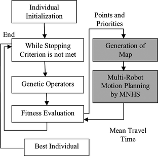
The basic approach used in the algorithm is genetic algorithm (GA). In this approach we use GA to generate a set of points in the entire robotic map. This set of points represents characteristic points that any of the robots might find fruitful for using in their paths from source to goal. The fitness function of the GA is a specification of the usefulness of these points in carrying effective motion planning. Hence, we use MNHS-based motion planning for evaluating these points generated by the GA. The points are first converted to a graph to find the feasibility and distance between the various points. This graph is then given as input to the MNHS algorithm to carry out motion planning. The MNHS algorithm considers all the robots one by one according to their priorities, which is information embedded in the genetic individual. The paths of earlier planned robots serve as obstacles for the later robots. The various phases of the algorithm are discussed in the next subsection. The general algorithm is given in Figure 1.

FIGURE 1 The general structure of the algorithm.

General Algorithm

The entire algorithm is basically a GA, which gives it an iterative nature. The GA is responsible for making the algorithm return results even if the dimensionality of the map is reasonably high. The algorithm tries to identify good points in the map, which are later judged by the MNHS algorithm by carrying out planning with the given robots and constraints.

The first task in the implementation of the GA is the individual representation scheme. We assume that there are a total of β points in the map whose placement the GA is supposed to optimize. All these are embedded one after the other in the applied individual representation. The other task that the GA optimizes is the individual priorities of the various robots. There are N robots, each having a certain priority. Let the individual be represented by . This means that there are a total of 2 β +N genes in the individual. The first 2β genes correspond to the β points each with the x coordinate value followed by the y coordinate value. Hence, the points represented in the individual may be taken as . These points must necessarily lie within the map. Hence, 1 ≤ ≤ m and 1 ≤ ≤ n for all 1 ≤i ≤ β. Further, the priorities are given by Z ₁, Z ₂, … Z _N with 0 ≤Z _i  ≤ 1. Here, the rank of Z _j in the total vector Z ₁, Z ₂, … Z _N denotes the priority of j ^th robot.

The implemented approach uses a number of evolutionary operators that generate the higher-generation population from a lower-generation population. Uniform stochastic selection scheme is used for the selection of the fitter individuals. Here, the various individuals are placed at a roulette wheel with the circumference of the wheel being proportional to the expectation values. The wheel is spun once with c pointers, where c is the number of individuals to be selected. The expectation values are assigned to the individuals by the scaling operator. We use a rank-based scaling in which the expectation value of the individual is proportional to its rank. The other major operator of use is crossover in which we use a scattered crossover technique. In this technique, half of the genes are randomly taken from the first parent and the other half of the genes are taken from the other parent. This results in two children that go to the next generation of a population. The other operator used is mutation. In this algorithm we use a Gaussian mutation technique; the individual genes are changed by an amount that is obtained by a Gaussian probability distribution. The last operator of use is elite. Using this operator we directly transfer the best individual of one generation directly to the higher generation.

Fitness function in GA measures the usefulness of a solution or individual. In this algorithm, we take the fitness function as the average time taken by a robot to reach the goal from the source. A penalty proportional to the last point visited by the robot was added if the robot failed to reach the goal. Let L _i be the last point reached by the robot R _i . Let T _i be the time of travel of the robot. Further, let C _i be the speed of the robot. Fitness is given by

Here, Pen is the penalty constant.

Conversion to Graph

The GA works over a set of points, which may be easily converted from their genotypic representation to the equivalent phenotypic representation, which is a set of points in the map (along with priority values of robots). The MNHS, on the other hand, works over a well-defined graph. Hence, before hybridizing the two algorithms, which is the motive of this paper, we need to convert the set of points into a graph.

Let the graph be defined by G(V, E) where V denotes the vertices and E denotes the edges. We have a collection of β points in the map given by the GA P ₁, P ₂, … P _β. We add all the sources and goals of all the robots to these points S ₁, S ₂, … S _N , and G ₁, G ₂, … G _N . The resultant point set of the graph algorithm, hence, becomes

V consists of a total of 2N + β points. These points serve as vertices of the graph.

The next task to be performed is to compute the edges. An edge exists between any vertex i to any vertex j if the robot can travel from i to j without any collision with obstacles. The weight of the edge is taken to be the physical distance between the vertices i and j. However, travel between all the vertices may not be possible. It may be possible that travel between a set of vertices leads to collision. For this we travel across each and every point of the prospective edge and check for the existence of an obstacle. The edge is said to be existing between the vertices if no obstacle is found by traveling between the edges. Hence, the set of edges is given by

For algorithm working we use the adjacency matrix method of representation of the graph. This consists of a square matrix of size v × v, where v is the number of vertices in the graph. Every row/column of this matrix corresponds to a vertex in the graph. Any cell of the matrix a _ij denotes the existence of an edge between the vertex i and j. The cell stores NULL if no edge exists between the vertices. In case an edge exists, the value of the weight of the edge is stored in the cell. Because this is an undirected graph, hence a _ij  = a _ji . Also, the diagonal elements are all kept as NULL.

The major problem is that the total number of vertices in the graph may be very high. An edge is possible between any two vertices, which need to be checked for feasibility by the algorithm. The entire computation can take a great deal of time. For this reason, we propose the use of momentum for faster computation of path feasibility (Kala, Shukla and Tiwari 2010).

The concept of momentum states that a robot may not check for the feasibility of path by traveling at each and every point in it. It may rather check the path by a vague manner, whereby the vagueness is measured by the momentum factor o. For computation of the feasibility of a path, the robot checks the end points for feasibility, as well as every o ^th point on its way. Hence, for checking the feasibility of an edge between P _i and P _j , the following points would be checked.

k = 0, 1, 2, 3…, ∥ P _j – P _i ∥. is a unit vector from P _i in the direction of P _j .

We follow a coarser-to-finer strategy in this algorithm for the computation of feasibility. It is expected that most probably the infeasible paths would be left out by a coarser level of infeasibility computation and very few paths might need a finer level of feasibility computation. Hence, a great deal of time is saved by the algorithm. The first feasibility check is carried out with a very high value of momentum. If an edge passes this feasibility check, the check is repeated with a middle value of momentum. In case an edge passes this check as well, we set the value of momentum as unity and re-check the feasibility. If such a case each and every point in the path is checked. Hence if an edge passes this check, it is stated as feasible.

MNHS

The MNHS for the multirobots works on this graph for carrying out the motion planning and computing the paths of the individual robots. Here, we first deal with the application of MNHS for a single robot and later extend the same to work over multiple robots with known priorities.

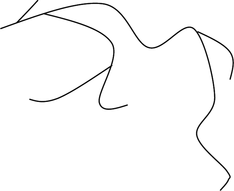
The advantage of MNHS for a robotic path problem over the conventional A* algorithm is very relevant to the problem of motion planning (Kala, Shukla and Tiwari 2009a). The A* algorithm may fail in maze-like maps, which are prone to sudden blockages near the goal. This situation may be found in complex robotic maps, which happen to be like mazes. The MNHS algorithm expands a large number of nodes, even those with poor costs. This ensures that if heuristics happen to drive the algorithm in the wrong direction, there are backup paths available. This has a multiplying effect on the time complexity, but in return is an assurance in case of the rapid blockage on the main path. The concept is shown in Figure 2. Here, the best path has almost reached the goal. At the same time, the other paths have been expanded to a reasonably good degree and are ready to provide a backup. The obstacles have not been shown in the figure.

FIGURE 2 The path exploration by multi neuron heuristic search.

The major task involved in the implementation of a single-robot MNHS is to formulate the cost function that drives the algorithm to find the goal starting from the source, given the robotic graph. The historic cost for the algorithm is simply the time from the source to the presently visited position. However, we also need to consider the possible necessity of smoothing the path. This means that every vertex visited must have enough distance from the various obstacles nearby. We hence penalize points from lying too close to the obstacles by adding a small penalty to their costs. This penalty varies with the distance from the obstacle in a Gaussian manner. This means that the cost is very high if the point is adjacent to the obstacle, but sharply decreases as we move. The heuristic cost of any point is simply the possible time of travel to the goal, if travel is in a straight line with uniform velocity.

Hence, consider planning the path of any robot R _a . The historic cost when traveling from any vertex P _i to vertex P _j is given by

Here, pen(P _j ) is the penalty function given by

Here, d is the distance from the closest obstacle, and is the factor that makes the penalty function comparable to the other costs. The heuristic cost is given by

The total cost is the sum of historic and heuristic costs.

It may be easily seen that after decent values of distance from an obstacle, the penalty factor would decrease to 0. Hence, we compute the penalty factor only for points that lie close enough to some obstacle. The values of d to various points are precomputed and stored in a distance matrix D. This avoids repetitive computation for the various points in the evolutionary approach. This is done using the principles of dynamic programming, whose recurrence relation and initial condition is given by

where k is the dynamic programming iterator, and δ(P _j ) is the neighborhood function that returns all points in the neighborhood of P _j (the 8 surrounding points).

The search always starts from the source and continues until the goal is found, per the conventional working methodology of the MNHS. This solved the problem of planning for a single robot using MNHS.

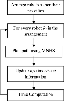
However, the problem we deal with is that of multirobot motion planning. For this we need to plan the path of multiple robots from their starts to their destinations. This can be done by processing each robot one by one according to the priorities returned by the GA. Hence, we take one robot, plan its path, and then proceed with the other robots. This process is given in Figure 3.

FIGURE 3 MNHS planning for multiple robots.

The set of priorities is already given, based on which we may compute the ranks of every robot. The robots are processed in a strict rank-based order, starting from the robot with a higher priority or a higher rank.

The entire discussion about walking through a potential edge and figuring out its feasibility and later making the adjacency matrix is applicable for the static obstacles in the path. The entire map we have in hand, however, contains the moving robots as well, which need to be avoided in the journey. The information about the moving obstacles is, however, not available at the time of making the graph. Because the robots would be planned by the MNHS, their trajectories would be known, and these would later be known as mobile obstacles to the graph. Hence, the only change to be applied in the MNHS algorithm is that before processing any edge e _ij , it must check for its feasibility.

We hence place a provision of a data structure called time-space for all the robots whose paths have been computed as they had higher priorities. This data structure is of the form {L _b (t)}, which returns the position of the robot R _b at time t. Assume that the robot enters the vertex V _i at a time t _i . The robot now intends to take edge e _ij for going to vertex V _j . The total time interval during which the robot stays within the edge is given by

Let L _a be the physical location of the robot at any time t during this time interval. The position is given by

The edge e _ij may be considered feasible by the robot R _a for its planning, if there is no collision of this robot with any other robot that has already been planned. Hence, e _ij is feasible if

Here, inequality means that neither of the locations is same, nor are the two robots R _a and R _b near to each other with consideration to their lengths and breadths. We further state that the two robots must have an additional safety margin between them for easier navigation. If an edge is infeasible, it may not be processed. The various costs discussed remain the same. The other task to be carried out is the updating of the space-time graphs, where we need to add the information about the planned robot, once it is available after the planning process. The MNHS algorithm for any robot R _a returns the set of vertices traveled (in order) by the robot. The time information is maintained for all the vertices in the implementation used by the algorithm. This helps in computation of the edge feasibility. Hence, the search algorithm gives as its output the set {S _a (0), P ₁(t ₁), P ₂(t ₂)… P _k (t _k ), G _a (t _{k +1})} denoting the visited vertices and the corresponding time. For every pair of vertices <P _i (t _i ), P _{i +1}(t _{i +1})> in the set, we update the corresponding space-time graph of the planned robot by adding L _a (t) to the space-time graph (given by Equation (11)) for all t _i  ≤ t ≤ t _{i +1}. In this manner we may extend the motion planning to motion planning of multiple robots using MNHS.

Relation Between Genetic Algorihtm and MNHS

In this approach we primarily fused two well-known algorithms for the purpose of motion planning of mobile robots. This fusion was inspired from the study of the basic advantages and disadvantages of the two algorithms. We intended to fuse these algorithms in a manner that one algorithm eliminates the disadvantages of the other algorithm. In this manner the advantages are likely to be amplified, whereas the disadvantages diminish.

The MNHS is a graph search algorithm. Hence, it is very good in completeness and path optimality. This means that it is able to find out solutions to the problem, if they exist. Further, these solutions are optimal in nature because the algorithm considers virtually all possible cases before returning a solution. The A* algorithm, however, demands the map as well as the possible moves of the robot to be discrete. This puts a great limitation on the possibilities of flexible paths. A solution may be to drastically increase the number of possible moves, which means a very large number of edges for every vertex in the map. This, however, plays with the computational and memory costs. Further, the MNHS being a graph search algorithm may not work for maps of a very high resolution. In such a case, there would be too many vertices and edges, which might result in too many computations required for solving the complete map. The number of nodes in the open list may further become very large, disobeying the memory limits. Because it is not an iterative algorithm, we cannot break its run to get the path. This makes it impossible to use MNHS or other heuristic algorithms in most real-life scenarios.

The GA is the other algorithm used for fusion. This algorithm is an iterative algorithm that works over a probabilistic approach. These algorithms can work very well over high-resolution maps. Because the approach is iterative, we may need to stop the algorithm at any stage in order to use the results for robotic movements. However, these algorithms are not complete. These algorithms fail in a number of scenarios such as the narrow corridor problem in which the optimal path is found by navigating through a narrow corridor. These algorithms may be adapted to give results within a specific threshold of time. The results, however, may not be optimal in nature.

The role of the GA is primarily to eliminate the stated disadvantages of the MNHS. MNHS cannot work over high-dimensional maps, and hence, the task of reduction of dimensionality is carried out by the GA, which selects the good points and gives them as the inputs to MNHS. The other advantage includes the iterative nature and the probabilistic approach. The MNHS contributes by enabling the EA to generate only a pool of points with no knowledge of their interconnectivity and the final path that they form. This is a lot simpler problem compared to the problem of figuring out the exact path for each of the robots.

Hence, using the combination of both of these algorithms solves the twin problem of path optimality and time. It may be easily seen from the algorithm that the mutual contribution of the two algorithms is controlled by the factor β. On one hand, if β is very small, the resultant algorithm would be dominated by GA. The MNHS would have very little choice between the nodes selection. On the other hand, if β is very large, the algorithm would be primarily MNHS in nature. The placement of nodes would lose importance as compared to the path formulation between them.

RESULTS

The entire algorithm was implemented in MATLAB platform. The map was made using the paint utility and was saved in an image file. This was imported in MATLAB, which was directly used as the algorithm map function. In all the experiments, we used a map of size 500 × 500 pixels. The map was first preprocessed for computation of the distances of the various points from the obstacle using the dynamic programming concept explained earlier. The entire map along with these precomputed values was later used for the GA evolution of the robotic path. The GA worked over the generation of the path using its evolutionary principles. The modules of conversion to graph and of multirobot MNHS graph search were also coded as MATLAB modules. The entire algorithm was executed for a number of scenarios, which were followed by execution for the analyses of parameters.

The first scenario given to the algorithm consisted of a map with irregular objects scattered all around. Four obstacles were taken at the four corners of the map. To create a challenging problem, the goals of these robots were specified as the opposite corners. It is natural that the resulting optimal path would be the same for the two robots at opposing corners. Hence, this scenario even tests for the cooperation factor among the robots. The initial configuration including, lengths, widths, sources, goals, and speeds of the robots is given in Table 1. The GA used had a population count of 15 individuals. The algorithm was executed for a total of 10 generations. The crossover rate fixed for the algorithm was 0.7. Elite count was 2. The value of the number of points to be optimized by the GA β was fixed to 30. The algorithm took about 13 minutes for the optimization. The time taken by each robot is given in Table 1. The path traced by the robots at different instances of time is given in Figure 4. The same is illustrated in Video 1.

FIGURE 4 Positions of the robots and the trajectory traced at various instances of time for first scenario. (Color figure available online.)

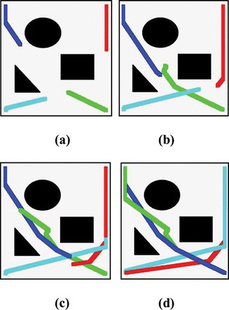
TABLE 1 Statistics of Various Robots for Scenario 1

S. No.	Property	Robot 1	Robot 2	Robot 3	Robot 4
1.	Length (pixels)	15	15	15	15
2.	Width (pixels)	15	15	15	15
3.	Speed (pixels/unit time)	1	1	1	1
4.	Source	(22, 22)	(477, 477)	(22, 477)	(477, 22)
5.	Goal	(477, 477)	(22, 22)	(477, 22)	(22, 477)
6.	Travel Time	686	722	818	814
7.	Length of path	686	722	818	814
8.	Reached	Yes	Yes	Yes	Yes
9.	Collisions	No	No	No	No

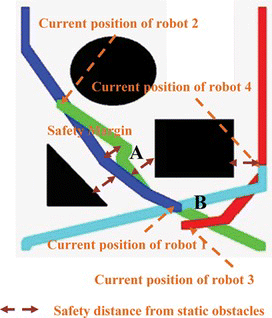
Based on the presented images and the video, it may be easily observed that in the entire duration of the journey, every robot tried to maintain a comfortable distance from each other as well as the static obstacles. The distance included keeping a safety margin for the validity of the nonholonomic constraints at the time of path smoothening. This distance was kept in the case of the walls and other static obstacles. For distance from the other robots, only a safety margin was kept. It may be further observed that the extra margin from the walls is only a desire and not a mandatory requirement. Sometimes the robot may have to go quite near to the obstacles, as in other cases the optimality of the path may be drastically lost. Figure 5 shows the distances that each robot maintained from the other robots as well as the static obstacles. A distinctive case can be seen from the path of the second robot (shown in green) which deviated from its path at point A to allow the first robot (shown in blue) to pass by. This was a kind of overtaking mechanism generated purely by the evolutionary approach. In another case it may be easily seen that the first robot (shown in blue) and the third robot (shown in red) tried to adjust their positions of turn so that they did not collide with each other at point B. This is an example of coordination in which the two robots are quite distant from each other. A similar trend can be seen with the fourth robot (shown in cyan) and the third robot (shown in red). Hence, the algorithm by its evolutionary process caters to the need of complex coordination among the robots. This is done by the optimization of the priority values.

FIGURE 5 The safety margins and distances maintained by the robot with other robots and obstacles. (Color figure available online.)

The other scenario we give is of regular-shaped obstacles with a higher number of robots. The number of robots was increased to six. We placed additional robots across the center of the top and bottom side of the map. The values of the various parameters were kept constant as discussed in the earlier scenario. The algorithm in this case also produced optimal results. The sources, goals, and other information about the scenario are given in Table 2. The trajectory followed by the robots at various times is given in Figure 6. The complete path traced by the robot is given in Video 2.

FIGURE 6 Positions of the robots and the trajectory traced at various instances of time for second scenario. (Color figure available online.)

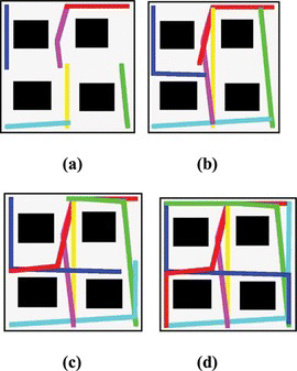
TABLE 2 Statistics of Various Robots for Scenario 2

S. no.	Property	Robot 1	Robot 2	Robot 3	Robot 4	Robot 5	Robot 6
1.	Length (pixels)	15	15	15	15	15	15
2.	Width (pixels)	15	15	15	15	15	15
3.	Speed (pixels/unit time)	1	1	1	1	1	1
4.	Source	(22, 22)	(477, 477)	(22, 477)	(477, 22)	(22, 250)	(477, 250)
5.	Goal	(477, 477)	(22, 22)	(477, 22)	(22, 477)	(477, 250)	(22, 250)
6.	Travel Time	900	858	844	880	464	457
7.	Length of path	900	858	844	880	464	457
8.	Reached	Yes	Yes	Yes	Yes	Yes	Yes
9.	Collisions	No	No	No	No	No	No

This is another scenario in which we saw a great deal of coordination among the robots. There were few basic paths in which the robots could move, that is, the path around the circumference of the map and those joining north to south and east to west. According to design, the passages were not wide enough to accommodate two robots simultaneously, but were wide enough that they may just fit in. There was no means by which three robots could lie parallel to each other. In this case, we see that, to a large extent, the robots chose to move close to the static obstacles in order to arrive at shorter paths. This can be seen in the path of the fifth robot (shown in pink), which happened to remain reasonably close to the obstacle at the top left of the map, in order to allow the sixth robot (shown in yellow) to pass by with some decent distance from obstacles and from the other robot at the time of passing. The other robots starting their journeys at the four corners chose to maintain a comfortable distance from the static obstacles. These hence decided to use available pathways such that no two robots happen to be in the same pathway at any point of time. This enabled them to keep sufficient distance from the static obstacles. The first robot (shown in blue) had to keep a low distance from the top-left obstacle as the map did not allow it to smoothly pass through using any path. All its moves started with narrow separation from the obstacle. This again ensured that keeping large distances from the obstacles is desirable and not mandatory.

The last scenario we gave for the testing of the system was to test the effect of multiple speeds. We used two robots with different speeds for the experimentation. The source of the first robot was the top-left corner, which was the goal of the second robot and vice versa. The map used for this purpose had two broad passages between the source-goal pairs. The passages were large enough to accommodate smooth travel of one robot per the safety restrictions and the robotic dimensions. However, these were kept narrow enough so that these could not be occupied by both robots simultaneously, considering all safety distances between any pair of robots and obstacles. The scenario is completely described in Table 3. The parameters of the algorithm remained unchanged. The trajectory of the robot at various instances of time is given in Figure 7. The complete trajectory is given in Video 3.

FIGURE 7 Positions of the robots and the trajectory traced at various instances of time for third scenario. (Color figure available online.)

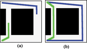
TABLE 3 Statistics of Various Robots for Scenario 3

S. no.	Property	Robot 1	Robot 2
1.	Length (pixels)	15	15
2.	Width (pixels)	15	15
3.	Speed (pixels/ unit time)	2	3
4.	Source	(22, 22)	(477, 22)
5.	Goal	(477, 22)	(22, 22)
6.	Travel Time	542	627
7.	Length of path	1084	1881
8.	Reached	Yes	Yes
9.	Collisions	No	No

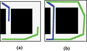
Here it may be easily seen that the faster robot chose to travel by the longer path, making the shorter path available for the smaller robot. This made the average time of travel fairly low, because the time would have been very high had the slower robot traveled by the longer path. We reversed the speeds and found that the trend reversed as well. Now the robot initially located at top-left corner, and moving with slower speed in this case, preferred to take the smaller path, making the other path available for the robot initially located at the bottom-left corner. This is shown in Video 4 and briefly shown in Figure 8.

FIGURE 8 Positions of the robots and the trajectory traced at various instances of time for reverse of third scenario. (Color figure available online.)

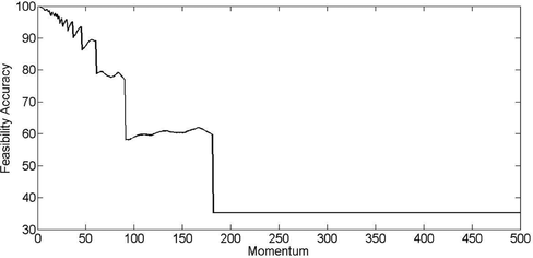
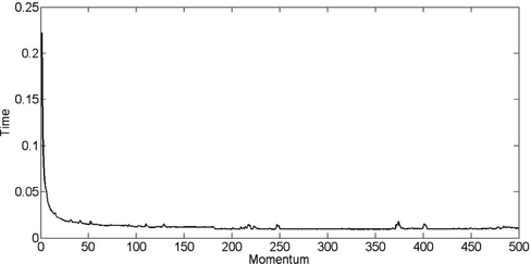
The other task that we carried out was to study the effect of momentum that controls the vagueness with which a path is checked for feasibility on time and to compare the results with the actual path feasibility. We used the same map that had been used for the experimentation of the second scenario. We generated a total of 50,000 paths from randomly generated sources and having random goals. We checked the feasibility of the path by a number of values of the momentum, from large values to small values. The execution time for each was noted. We further checked whether the decision produced regarding the feasibility of the path was correct. By repeating the experimentation on a number of robotic paths, we obtained the mean execution time and percentage accuracy of feasibility prediction for every value of momentum. The graph so produced for various values of momentum is given in Figure 9 and Figure 10.

FIGURE 9 The relation between momentum and the feasibility prediction accuracy.

FIGURE 10 The relation between momentum and the execution time.

It may be easily seen that as we increased the momentum, the accuracy of feasibility prediction decreased. Hence, the higher values are unlikely for accurate prediction of feasibility. On the other hand, the algorithm shows a 100% correct prediction at a value of unity for momentum. This is because each and every point in the graph is checked. The same results may be observed in Figure 10, showing the relation of momentum with time. As we increased momentum, fewer points were checked for feasibility, and the time of execution hence was reduced. We saw a sharp decrease in execution time in the region from momentum value of 0 to a momentum value of 50. It may be seen that this is exactly the region where we would operate, because below this value the predictive capability of the algorithm is too low. Both these graphs have some randomness that can be seen, which is a result of the generation of random paths.

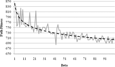
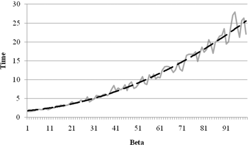
The other analysis we carried out was to check the working of the number of random points generated in the map optimized by the GA β. Again, for experimentation we used the second scenario with the same robot positions and speeds. For a large number of values of β, we generated random points and found the path length of the robots computed by the algorithm. For every value of β, this experimentation was repeated 20 times, and the minimum value of path length was taken. This eliminated the effect of poor points being generated in the map, which is a likely condition, especially with lower values of β. For computation of the time we took the mean of 20 runs. The resulting graph is given in Figure 11. The time of execution required in each of these cases is given in Figure 12.

FIGURE 11 The relation between path fitness and β.

FIGURE 12 The relation between time of execution and β.

In both these figures, the general trend of the algorithm is shown by adding trend lines. It may be seen that for every observation the algorithm generates random β points and then solves the map using these points. This gives randomness to the algorithm, which is responsible for visible oscillations in the graph. The plotted trend line shows the mean trend of the effect of the factor. It may be easily seen from the figures that increasing β results in generation of a larger number of points on the graph. This means the possibility of generation of more flexible paths, which may be smooth and have shorter lengths. Further, as we increase the number of points, it is more likely that some of these points would lie close to the ideal points for optimal motion of the robots. Hence, as we increase β, the path length further decreases and so does the total dependency of the algorithm on GA. For very large values of β there is hardly any improvement because the algorithm is easily able to generate paths around their ideal values. Increasing points hence has not much improvement. However, the same produces an increase in computation time. When this framework is put over GA, it would mean a larger overhead in time, which would mean restricting its number of individuals and generations.

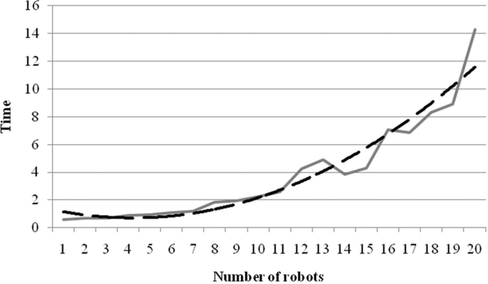
The last experiment was carried out to check the relation between the number of robots and time of execution for the algorithm to compute the paths between their source and their goals. Here, we randomly generated a number of robots with random sources and goals. The time required to make the graph and compute the path using MNHS was measured. The experiment was repeated 20 times and the mean execution time was noted. The resultant graph is shown in Figure 13.

FIGURE 13 The relation between time of execution and number of robots.

The figure shows the increase in the time of computation of the paths as we increase the number of robots. Again, the oscillations and the irregular trends are because of the random generation of the source positions and the goal positions. The trend line plotted shows the general trend. The increase in the number of robots means that there is a general increase in time; planning is done one after the other for different robots, which accounts for the linear increase in time. Further, the robots need to check for the paths of the other robots having higher priorities before going through any edge, which accounts for the higher increase in time complexity.

CONCLUSIONS

In this article, we proposed an interesting method of motion planning of multiple robots based on fusion of GA and MNHS. The advantages and disadvantages of both these methods were identified, which motivated the fusion such that the individual disadvantages are removed and the advantages are combined. By this approach we intended to plan the paths of multiple robots of different sizes and capable of moving with different speeds. The GA tried to generate a large number of points on a two-dimensional map that clearly stated the obstacles and the paths where the movement could be made. The GA further tried to generate a priority strategy by which every robot has a priority governing its order in the planning process. The planning was done using the MNHS search algorithm in the prioritized manner. The planner ensured that the newly planned robot does not collide with any of the prior planner robots. The cost function of the MNHS was modified to ensure that the robot tries to keep some minimal distance from all the obstacles and the other robots that have higher priorities. This could make the entire cost function of the algorithm very heavy and computationally expensive. For the same reasons, we used the concept of momentum, with which the feasibility of the path is checked at selected points, in place of a point-by-point search that may be computationally expensive. We looked up the path for feasibility for a varying degree of momentum. The last level is the finest level, ensuring correct reporting of the results.

The approach involved a number of experiments. In the generated scenario over which the approach was implemented, the paths were seen to be optimal. The algorithm not only succeeded in generating small paths that took shorter time for travel of the robot, but the robot was able to avoid the obstacles and the other robots by significantly large margins. This ensures that these paths may be very easily smoothened to obey nonholonomic constraints. Further, smoother paths would enable the robot to travel at higher speeds, making the travel duration shorter. We further studied the planning of the robots with different speeds, and observed that the planner enabled the robots to arrange their priorities per their speeds, in order to make the total work plan of the entire algorithm optimal.

The analysis of the various factors was done, which is important from the perspective of setting the correct parameter value per the requirements of the scenario. The plotted relations between the parameters were more or less on the expected lines. On one hand, the increase in momentum displayed a decrease in the time requirements to compute the path feasibility. On the other hand, it resulted in a poor measure of feasibility because the infeasible paths could be reported to be feasible. The same relation was seen with the number of points to be optimized by the GA β. The higher number of points showed a general trend to be able to generate optimal paths. However, the computational time also increased as we increased the number of points. The increase in the number of robots also showed an increase in the computation time.

The presented algorithm may be regarded as an improvement over the conventional graph search algorithms as well as the conventional evolutionary approaches for the problem of multirobot motion planning; it eliminates the individual limitations of the two approaches. The implemented approach enables the generation of more flexible paths, which add to optimality as well as iteration to work over the high-resolution graph from the point of view of graph search approaches. The implemented approach is an improvement over the GA approaches using prioritized planning (Bennewitz, Burgard, and Thrun 2001, 2002; Carpin and Pagello 2009), because the planner in this approach may evolve a set of points in any order, unlike the other approaches in which the points need to be in the same order as the path in order to be traversed by the robot. This makes evolution a lot easier. The discussions to a large extent may be generalized to a number of hierarchical/hybrid graph search algorithms (Cagigal and Abascal, 2005; Kala, Shukla, and Tiwari 2011b), in which the discreteness of the path is still an issue, as well as the other hierarchical/hybrid GA (Kala, Shukla and Tiwari 2010), which still have a difficult evolution because of the problem complexity. The fusion of the two algorithms enables better evolution and the generation of optimal paths.

Although the algorithm has a number of advantages, there are some limitations that need to be addressed in the future. The decision over the optimal value of β and the momentum is critical, which is not done by the algorithm. It may be possible to make these parameters adaptive so that they tune themselves as the algorithm proceeds. Further, the algorithm needs to be implemented and verified over real robots. This would raise more practical issues in its usage. Being primarily an evolutionary approach, the algorithm does not consider the presence of dynamic obstacles that may be likely in real-life scenarios. Further, we just produce a provision for smoothening of the path, which is not done by the algorithm. Making a provision of path smoothening inside the fitness function may enable generation of better paths and an anomaly between path length and its smoothness. All these issues may be dealt with in the future.