
Abstract
Homicide is one of the most serious kinds of offenses. Research on causes of homicide has never reached a definite conclusion. The purpose of this article is to put homicide in its broad range of social context to seek correlation between this offense and other macroscopic socioeconomic factors. This international-level comparative study used a dataset covering 181 countries and 69 attributes. The data were processed by the Self-Organizing Map (SOM) assisted by other clustering methods, including ScatterCounter for attribute selection, and several statistical methods for obtaining comparable results. The SOM is found to be a useful tool for mapping criminal phenomena through processing of multivariate data, and correlation can be identified between homicide and socioeconomic factors.
INTRODUCTION
Homicide is an offense of one person illegally depriving the life of another person. Among all offenses punished by law, homicide is one of the most serious and attracts global attention (United Nations Office on Drugs and Crime Citation2011). Exploration of fundamental causes of crime proved to be a nearly impossible task, because crime is always complicated, usually secret, concealed, and underreported. Distribution of crime differs among geographical units, among demographical groups, and among socioeconomic combinations. Different combinations of demographical or socioeconomic factors have played a significant role in the study of crime (Rock Citation1994).
To deal with a broad range of socioeconomic factors, the study of crime requires data mining and visualizing techniques, which have broadly shown their practical value in various domains. The self-organizing map (SOM), using an unsupervised learning method to group data according to patterns found in a dataset, is a qualified tool for data exploration. The interconnection between artificial intelligence and the study of crime makes an innovative study possible.
Currently, the SOM has been used in identifying individual offenses; for instance, the detection of credit card fraud (Zaslavsky and Strizhak Citation2006), automobile bodily injury insurance fraud (Brockett, Xia, and Derrig Citation1998), burglary (Adderley Citation2004; Adderley and Musgrave Citation2005), murder and rape (Kangas Citation2001), homicide (Kangas et al. Citation1999; Memon and Mehboob Citation2006), network intrusion (Leufven Citation2006; Lampinen, Koivisto, and Honkanen Citation2005; Axelsson Citation2005), cybercrime (Fei et al. Citation2006; Fei et al. Citation2005), and mobile communications fraud (Hollmén Citation2000; Hollmén, Tresp, and Simula Citation1999; Grosser, Britos, and García-Martínez Citation2005). These are the main areas where the application of the SOM has previously been emphasized in the research related to criminal justice.
There is a general lack of research to be found on macroscopic aspects of criminal phenomena (in this article, homicide in particular) as related to socioeconomic factors. The current situation created a motivation for designing experiments using the SOM, compared with and supplemented by other methods. Applying the SOM to investigate correlation between homicide and a broad range of socioeconomic factors, this article represents an effort to innovatively apply the SOM to the study of homicide, previously unattempted by many other studies.
METHODOLOGY
This study applies the SOM, developed by Kohonen (Kohonen Citation1979), to cluster and visualize data. It is an unsupervised learning mechanism that clusters objects having multidimensional attributes into a lower-dimensional space, in which the distance between every pair of objects captures the multiattribute similarity between them. On processing the data, maps can be generated using software packages. By observing and comparing the clustering map and feature planes, it is possible to identify distribution of homicide among different socioeconomic factors and correlation between homicide and socioeconomic factors. Detailed correlation tables can also be realized automatically with Viscovery SOMineFootnote1 which adopts the correlation coefficient scale ranging from −1.0 to +1.0. These results, including clustering maps, feature planes, and correlation tables constitute the fundamental ground for further analysis.
Although every attribute can be used by the SOM in clustering, their roles in the clustering are not evaluated. In order to select attributes, ScatterCounter (Juhola and Siermala Citation2012a, Citation2012b) will be used to measure the separation powers (between clusters) of all attributes. Those that have weak powers will be dropped from the dataset, and the reduced dataset will be used in final processing and analysis. For concrete formatting of data, a difference between using the SOM and using ScatterCounter is that the SOM can process missing data by marking them as “NaN” (Not-a-Number), whereas the ScatterCounter can be used only when the missing data in the original dataset are substituted with real values. In this research, missing values are imputed by the medians of other available values of the same attributes in the same clusters.
In addition to the SOM, k-means clustering, discriminant analysis, k-means nearest neighbor classifier, Naïve Bayes classification, Decision trees, Support Vector Machines (SVMs), Kruskal–Wallis test, and Wilcoxon–Mann–Whitney U test will be used to validate the clusters and analysis by calculating how accurately these methods put the same countries into the same clusters as the SOM does.
DESIGN OF EXPERIMENTS
Countries Included
Included in the experiment are 181 countries and territories, coded in . These codes will be shown in the maps as labels. These countries were selected based on the availability of data on selected attributes. Most of these countries are members of the United Nations, which, however, maintains the database containing information from nonmember countries and territories. Usually, statistics of members are more available than those of nonmembers. But in exceptional cases, this is not true. Therefore, some members were dropped due to unavailability of data on a significant amount of indicators, although some nonmembers were kept because of their well-maintained statistical systems. Generally, the ratio of available data on indicators of individual countries or territories was controlled above 70%, and mostly above 80%.
Crime and Socioeconomic Factor
This study contains 69 attributes: one attribute, homicide per 100,000 people, is a crime-related indicator, whereas 68 others are socioeconomic factors. An overview of all attributes that were used in this study is given in . The selection of the contents of these indicators was primarily based on availability of data. Less consideration was put on the traditional concept of what might in actual fact cause the occurrence of offenses of homicide, because in this research predetermined and presumed correlations were temporarily ignored. Accordingly, in this research, some of these factors might traditionally be considered closely related to homicide, but
TABLE 1 Countries and Territories Included
TABLE 2 Country Socioeconomic Situation by 69 Attributes with Their Means, Standard Deviations, and Missing Values in Percent (Attributes in Bold Were Finally Removed According to Their Poor Separation Power)
The purpose of the current study was to find groups of countries and territories according to their homicide rate and to explore correlation between homicide and its socioeconomic context. In this study, the data source is the United Nations Development Program (UNDP) online database. In this original dataset, total missing values accounted for 6.80%. Ten of the attributes had no missing values, whereas missing values in other attributes ranged from 0.55% to 21.55% (see ). This criterion was similarly set as that of selecting countries and territories. As a result, in the final dataset, most columns and most rows were with the ratios of available data above 80%, with a few exceptions slightly below 80%.
Preprocessing and Attribute Selection
In the experiment, an important component was to preprocess the data with the SOM software and select attributes with ScatterCounter. The starting point was to generate clusters using the Viscovery SOMine, with which missing values did not need to be imputed as real numbers, instead they were marked as “NaN” only. Because four clusters were produced, the clusters were numbered as 1, 2, 3, and 4. These numbers were taken as cluster identifiers, which were used to mark countries and territories in a separate column. The dataset with countries and territories bearing the marks of cluster identifiers would be processed with ScatterCounter (Juhola and Siermala Citation2012a, Citation2012b). In this dataset, missing values were imputed by substituting them with medians of pertinent clusters, because this software package will not deal with missing values.
ScatterCounter is a software tool designed to evaluate how many “classes” (named “clusters” in the SOM) differ from each other in a dataset. The process starts from a random instance of a dataset and traverses all instances by searching for the nearest neighbor of the current instance, then the one found to be the current instance is updated and the whole dataset iterates. During the process of the search, every change from one class to another is counted. The more class changes there are, the more the classes of a dataset are overlapped.
To compute separation power, the number of changes among classes is divided by their maximum number and the result is subtracted from a value that was computed with random changes among classes, but keeping the same sizes of classes as in an original dataset applied. Because the process includes randomized steps, it is repeated five to ten times, and the average is used for separation power.
Separation powers can be calculated for the whole dataset or for every class and for every attribute (Juhola and Siermala Citation2012a, Citation2012b). Absolute values of separation powers are from [0,1]. They are usually positive, but small negative values are also possible when, in some classes, an attribute does not virtually separate at all. Considering that such attributes might be useful for some other classes, typically it needs to find those attributes that are rather useless for all classes so that these can be left out of the continuation.
Separation powers of attributes in each cluster and in the whole dataset are presented in . Although an attribute may have separation powers around zero for some clusters, if for one cluster its separation power is larger, it can be useful to separate this cluster from the others. Therefore, separation powers of each attribute were computed both cluster by cluster and for the whole dataset. With these results and observations, seven attributes (6, 8, 17, 18, 41, 63, 64) have poor separation powers and are removed from the dataset used in the following experiments and analysis.
FIGURE 1 Separation powers of each attibute in (a) cluster C1, (b) cluster C2, (c) cluster C3, (d) cluster C4, and (e) the whole dataset. The order of the 69 attributes from the left to the right along with the horizontal axis is that given in . Finally, seven attributes (6, 8, 17, 18, 41, 63, 64) with poor separation powers were discarded.
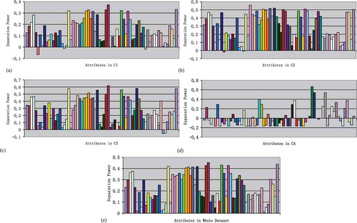
As a result, all the 62 attributes preserved in the dataset had stronger separation power and supposedly enable valid clustering. In this reduced dataset, missing values accounted for fewer than 7.32%. The rate of missing value was increased because the seven attributes were identified as having weak separation power and were discarded: three attributes with no missing value, three other attributes with the ratio of missing values below initial average, and the other attribute with the ratio of missing value below the attribute with the most missing value. Because the number of countries had no change, the ratios of missing values of reserved single attributes were the same as those in the original dataset.
Construction of the Map
In this study, the software package used is Viscovery SOMine 5.2.2 Build 4241. Compared with other software packages, Viscovery SOMine has almost the same requirements on the format of the dataset. At the same time, requiring less programming, it enables an easier and more operable data processing and visualization.
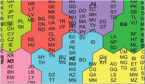
Here again, the dataset was formed from the original one by deleting attributes with weakest separation power. Missing values were marked with “NaN.” The SOMine software automatically generated maps from the dataset of 181 countries and 62 attributes. The clustering map () as well as some other detailed statistics, such as correlations as discussed following, can be used in further analysis.
FIGURE 2 Clustering map with cluster names C1–C7 and labels of countries.
Support Vector Machine, One-vs-One Method, and Parameter Estimation
Support Vector Machine (SVM; Vapnik Citation2000; Burges Citation1998; Cortes and Vapnik Citation1995) is a supervised classification method developed for two-class classification problems. The key idea in SVM is to construct a classes-separating hyperplane in the input space such that the margin (distance between the closest examples of both classes) is maximized. By this means, the generalization ability (in other words, the ability to predict the unseen test samples correctly) of an SVM classifier is the highest. When the classes in a dataset cannot be directly separated by a hyperplane in the input space, we need to use the kernel functions (Vapnik Citation2000; Burges Citation1998). The main point in kernel functions is that the training set, which is located in the input space, is mapped by a nonlinear transformation to (possibly) an infinite dimensional space where the classes can be separated by a hyperplane. The construction of a maximum margin SVM classifier is based on optimization theory, and because the basic theory of an SVM classifier is well known from the literature, a reader can find the detailed mathematical derivation from Vapnik (Citation2000), for instance. In this article, we applied least squares SVM developed by Suykens and Vandewalle (Citation1999).
Due to the two-class restriction of SVM, a different kind of approach for multiclass cases (the number of classes is greater than two) is needed. A one-vs-one (OVO) method (Galar et al. Citation2011; Joutsijoki and Juhola Citation2013, Citation2011) is a commonly used multiclass extension for SVM. In the OVO method, one classifier is constructed for each class pair. Thus, altogether, M(M−1)/2 classifiers are needed for an M > 2-class classification problem. Each of the classifiers gives a predicted class label (vote) for test examples. The final class label for a test example is the label that occurs most often. If a tie occurs among the classes, the final class label is solved by 1-nearest neighbor, as in Joutsijoki and Juhola (Citation2013, Citation2011).
The use of SVM requires estimation of parameters. In this study we applied seven kernel functions. These were: linear, polynomial kernels (degrees from 2 to 5), radial basis function (RBF), and sigmoid (see formulas Hsu, Chang, and Lin Citation2013). For the linear and polynomial kernels only one parameter (C, which is a penalty parameter) is to be estimated, for the RBF there are two parameters (C and γ, which is the width of the Gaussian basis function), and for sigmoid there are three parameters to be estimated (C, κ > 0, and δ < 0). We performed the parameter value estimation in the following manner. First, a dataset was divided into training and test sets with a leave-one-out method. Second, every training set was divided into training and test sets such that 1/3 was for validation and 2/3 for training. Third, SVMs were trained by using a smaller training set and the accuracy of the validation set was evaluated. Fourth, the average accuracy of validation sets was determined. Fifth, when the best parameter value combination was found (the highest mean accuracy of validation sets determined the best parameter values), SVMs were trained again by using the full training set and they were tested with the test set. Because the OVO method contains several binary SVM classifiers, we decided to simplify the test arrangements so that we used the same parameter values for every SVM classifier. We tested the linear and polynomial kernels with 26 parameter values (Cє{2−15, 2−14, … , 210}) and both RBF and sigmoid kernels with 676 parameter value combinations (C, γ, κ є{2−15, 2−14, … , 210} and δє{−2−10, −2−9, … , −2−15}). All the tests and implementation of the OVO method were made with MATLAB 2010b and the Bioinformatics Toolbox of MATLAB.
RESULTS
On processing of data, seven clusters have been generated, each representing groups of countries sharing similar characteristics. As a default practice in SOMs, values are expressed in colors: warm colors denote high values, cold colors denote low values.
In analyzing country homicide situations to fulfill different demands, when there are many objects involved, two other levels of clustering concepts, superclusters and subclusters, can also be used. Within the frameworks of each level of clusters, members in each cluster have their common properties based on where they were grouped and how they could be further analyzed.
Superclusters, Clusters, and Subclusters
Clusters are shown in . Due to the features of the software package, countries and territories are not all shown in the map. In order to give a full picture of these clusters, the following lists all the countries and territories in each cluster:
Cluster C1 consists of 23 countries: BR, CO, EC, IR, PE, SR, VE, ID, MY, TH, DZ, TT, RU, VN, AZ, BM, KG, KZ, MN, TJ, TM, UZ, BO
Cluster C2 consists of 26 countries: BY, CU, HR, LT, LV, ME, EE, HU, BG, CN, RO, AL, AM, BQ, GE, MK, RS, UA, AR, CL, CR, MX, PH, TN, TR, UY
Cluster C3 consists of 33 countries: GH, KH, CM, MG, NG, TG, BI, ET, KE, MW, MZ, RW, TZ, UG, CD, CF, CI, GN, GW, LR, SL, TD, BW, CG, GA, MM, NA, AO, GO, LS, SZ, ZM, ZW
Cluster C4 consists of 24 countries: IN, IQ, KM, PK, SB, TL, VU, BD, AF, BJ, DJ, GM, MR, PG, RE, SN, YE, LA, NP, SD, BF, HT, ML, NE
Cluster C5 consists of 30 countries: AG, BB, BS, GD, MD, MU, WS, BZ, FJ, GY, HN, JM, LC, MH, MV, TV, VC, CV, NI, ST, SY, TO, DO, LK, MA, PA, PY, SV, EG, GT,
Cluster 6 consists of 15 countries: BN, LI, AD, AE, BH, KW, LU, QA, SG, JO, LB, LY, OM, ZA, SA
Cluster C7 consists of 30 countries: ES, GR, IT, JP, PT, AT, AU, CA, DE, DK, FI, FR, GB, IS, NL, NO, NZ, SE, SI, US, BE, CH, CY, CZ, IE, IL, KR, MT, PL, SK
Compared with clusters generated by the software before several attributes were removed by applying ScatterCounter to select more useful attributes based on their separation powers, clusters here were to some extent regrouped. Principally, clusters before and after removing the attributes that had weak separation powers should have high similarity, including cluster numbers and countries in each cluster. This could be taken as the initial purpose for applying separation power.
Although the Viscovery SOMine software package provides the possibility for adjusting the number of clusters, and this can be used to set the same number of clusters for experiments before and after the application of separation power, usually automatically generated clusters represented the results that might have occurred the most naturally. In other experiments, the same number of clusters could be set deliberately; countries in these clusters were still regrouped slightly one way or the other. In this experiment, a more significant change of cluster number was still tolerated, because this was expected to leave a new space where the similar issue could be speculated.
By emphasizing difference between clusters before and after removing weak attributes by applying the separation power, it did not ignore the actual fact that a majority of countries that were originally in the same small groups (subclusters in clusters) were subsequently still in the same subclusters. That is to say, clusters changed, but the change took place primarily at the subcluster level, not the individual level. Single countries did not move from here to there separately. Rather, closely joined small groups of countries migrated from one cluster to another.
This phenomenon enabled research on small groups of countries on the background of the whole world by subtracting information from the SOM established by processing the data depicting the panoramic view.
Because the unsupervised clustering map and feature maps were generated based on 62 attributes, description of these clusters became more complicated. Particularly, when special information about one attribute is needed, countries and territories in these seven clusters may be better regarded as components in fewer numbers of superclusters. For example, according to the feature map of homicide rates (), these seven clusters can be seen as components in three superclusters:
Consists of cluster C3 (34 countries) and cluster C5 (30 countries). They have a higher level of homicide rate.
FIGURE 3 Feature map of homicide rate.
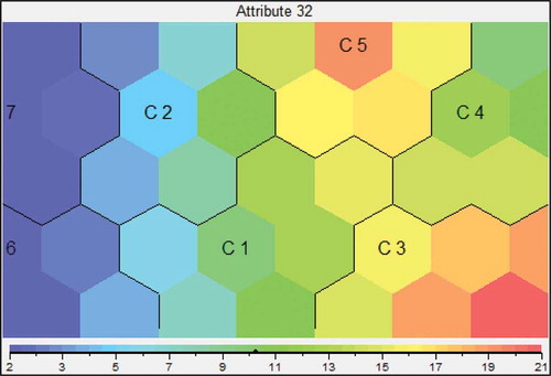
Consists of C1 (23 countries) and C4 (24 countries). They have a medium level of homicide rate.
Consists of C2 (26 countries), C6 (14 countries) and C7 (30 countries). They have a lower level of homicide rate.
Certainly, according to other attributes, there were more possibilities to form different superclusters, which would find their use in different research interests.
However, where necessary, within the frameworks of each of these seven clusters, several subclusters could also be identified. For a random example, in cluster 5, six countries, DO, LK, MA, PA, PY, and SV form a subcluster. It implicated that they have closer common properties than other members in the same cluster. Because they were closely grouped with each other, their clustering would not differ in feature maps of different attributes.
Although most countries were assembled in big or small groups, a few countries were isolated. They stayed separately far away from other countries, such as Bangladesh, Bolivia, and Indonesia. Although they have much in common with other countries in the same clusters, the map can still be used in a way to establish and elaborate diversity.
Validation of Clusters
A total of 181 countries times 62 attributes (after removing the poorest seven attributes identified by applying the ScatterCounter method) with original 7.32% missing values were imputed once again with cluster-wise medians, with new clusters (classes) given by the SOM clustering method.
After imputation, the results by the SOM were tested by several methods, including k-means clustering, discriminant analysis, k-nearest neighbor classifier, Naïve Bayes classification, Decision trees, SVMs, Kruskal–Wallis test, and Wilcoxon–Mann–Whitney U test (). True positive rates, in other words, percentage ratios of correctly classified countries and all countries were computed.
TABLE 3 True Positive Rates [%]
Unsupervised k-means clustering gave true positive rates between 36% and 41% when data were not scaled. Scaling of data made the results slightly better, between 45% and 46%. When data were standardized (attribute by attribute, by subtracting with the mean and dividing with the standard deviation of each attribute), overall results still bettered off, between 44% and 48%. Supervised k-means behaved worse than unsupervised, true positive rates are generally 4%–5% lower. In some cases, empty clusters also occurred.
Different methods of discriminant analysis were tested. Linear discriminant analysis got the same rate of 35.9% regardless of the data being scaled, unscaled, or standardized. Quadratic and Mahalanobis analyses got no positive definite covariance matrices, whereas logistic analysis got only 26.5% when data were standardized.
Furthermore, k-nearest neighbor classifiers (k-nn) gave results between 23% and 33% when data were not scaled, and 31.5% (k = 1, 3, 5, 7, 9, 11, 13) when data were scaled. When the data were standardized, results had a broader range, from 28.7% (k = 1) to 47.8% (k = 13).
Naïve Bayes with “normal” for distance function “dist” got a result of 38.7%, Naïve Bayes with “kernel” for “dist” got a result of 44.2%, decision trees got a result of 45.3%, regardless of data being scaled, not scaled, or standardized.
SVMs obtained the lowest rates when data were not scaled, but the highest rates when date was scaled, and medium rates when data were standardized (detailed in ).
The results of the Kruskal–Wallis test showed that there were significant (p < 0.05) differences among the groups defined by the clusters in 60 out of the total 62 variables. On average, six out of the 21 pairwise test results obtained with the Wilcoxon–Mann–Whitney U test were significant after the p values were corrected with the Holm’s method.
Correlations
Viscovery SOMine could generate a detailed list of correlations, based on which was created. Although even strong correlation between two attributes does not necessarily indicate causation, this will bring about materials for further analysis and reference. There are many opportunities for these results to be used to compare with previous studies on crime using other methods. Traditionally, single research on crime did not include so many attributes (or named correlation factors or causes). Even in textbooks, only a dozen or two were introduced. So it shall be highly anticipated to have such data mining methods available to process several dozens of attributes and to provide immediate reference for further analyses.
From , homicide was positively correlated with 23 attributes and negatively correlated with the other 38 attributes. Some correlation values were interesting, but others were very weak. Certainly, it is still too early to conclude what socioeconomic factors cause homicide, affecting its occurrence or its increase or decrease, especially when, more than ever before, this study included more factors than traditional research did in order to have full coverage.
TABLE 4 Correlations between Socioeconomic Attributes A and Homicide Rate (A32).
CONCLUSIONS
As one of the most serious offenses, the occurrence and distribution of homicide among regions in the world can be analyzed through accessible statistical data. This article dealt with macroscopic data for international comparison. Conventionally, analysis in the study of crime, either on general issues or on particular issues, did not handle large-scale multidimensional data. Specifically, when international comparison was carried out, discussion was quite abstract and theoretical, with lack of systematic data processing. By applying the Self-Organizing Map (SOM), this task was made possible.
With the SOM, multidimensional comparison was realized. The research objects, countries and territories, could be grouped into clusters of different levels: superclusters, clusters, and subclusters. Superclusters were useful to reveal common features of one or more attributes of research objects (countries and territories). They could be grouped in different ways with regard to different attributes. Clusters provided a primary basis for the analysis of distribution of countries and territories with all attributes in the dataset. Subclusters were used to investigate smaller groups of countries and territories within a cluster. In principle, countries and territories within a subcluster could be seen as having the most features in common in a socioeconomic context.
In fact, in the sense of the SOM, countries in subclusters were more closely joined together, forming a more stable structure than clusters. It was found that, before and after removing weak attributes by applying the separation power, the structures of clusters could be varied one way or the other. Countries in subclusters, however, could stay in a rather stable framework. In research on small groups of countries on the background of the whole world, it is a useful way to subtract comparative information from the SOM. It is also possible to situate individual countries, particularly those that are isolated on the map, in the international context.
By applying ScatterCounter to select attributes and refine the dataset, and by using k-means clustering, discriminant analysis, k-means nearest neighbor classifier, Naïve Bayes classification, Decision trees, SVMs, Kruskal–Wallis test, and Wilcoxon–Mann–Whitney U test to verify the SOM results, findings of the study gave additional proof that the SOM is an interesting tool for assisting research on individual types of crime. The clustering results were more easily visualized and more convenient to interpret, facilitating practical comparison among countries with diverse socioeconomic and criminal features. This article provides broad potential for applying data analysis and visualization methods in studies in the field of crime, where, in turn, researchers will find significant methodological value of this application.
FUNDING
The first author thanks the Tampere Doctoral Program in Information Science and Engineering (TISE) for financial support.
Additional information
Funding
Notes
1 Viscovery Software GmbH 2013, available at http://www.viscovery.net/somine/.
REFERENCES
- Adderley, R. 2004. The use of data mining techniques in operational crime fighting. In Intelligence and security informatics, Part 2, LNCS 3073:418–425. Berlin, Heidelberg: Springer.
- Adderley, R., and P. Musgrave. 2005. Modus operandi modelling of group offending: A data-mining case study. International Journal of Police Science and Management 5(4):265–276.
- Axelsson, S. 2005. Understanding intrusion detection through visualization (PhD thesis, Chalmers University of Technology, Göteborg, Sweden).
- Brockett, P. L., X. Xia, and R. A. Derrig. 1998. Using Kohonen’s self-organizing feature map to uncover automobile bodily injury claims fraud. The Journal of Risk and Insurance 65(2):245–274.
- Burges, C. J. C. 1998. A tutorial on support vector machines for pattern recognition. Data Mining and Knowledge Discovery 2(2):121–167.
- Cortes, C., and V. Vapnik. 1995. Support-vector networks. Machine Learning 20(3):273–297.
- Fei, B., J. Eloff, M. Olivier, and H. Venter. 2006. The use of self-organizing maps for anomalous behavior detection in a digital investigation. Forensic Science International 162(1–3):33–37.
- Fei, B., J. Eloff, H. Venter, and M. Olivier. 2005. Exploring data generated by computer forensic tools with self-organising maps. Proceedings of the IFIP Working Group 11.9 on Digital Forensics (2005)1–15.
- Galar, M., A. Fernández, E. Barrenechea, H. Bustince, and F. Herrera. 2011. An overview of ensemble methods for binary in multi-class problems: Experimental study on one-vs-one and one-vs-all schemes. Pattern Recognition 44(8):1761–1776.
- Grosser, H., P. Britos, and R. García-Martínez. 2005. Detecting fraud in mobile telephony using neural networks. In Innovations in Applied Artificial Intelligence, Lecture Notes in Artificial Intelligence, 3533: 613–615,ed. M. Ali and F. Esposito. Berlin, Germany: Springer-Verlag.
- Hollmén, J. 2000. User profiling and classification for fraud detection in mobile communications networks ( PhD thesis, Helsinki University of Technology, Finland).
- Hollmén, J., V. Tresp, and O. Simula. 1999. A self-organizing map for clustering probabilistic models. Artificial Neural Networks 470:946–951.
- Hsu, C.-W., C.-C. Chang, and C.-C. Lin. 2013. A practical guide to support vector classification (Technical report). Taiwan: National Taiwan University. Available at: http://www.csie.ntu.edu.tw/˜cjlin/articles/guide/guide.pdf.
- Joutsijoki, H., and M. Juhola. 2011. Comparing the one-vs-one and one-vs-all methods in benthic macroinvertebrate image classification. In Machine learning and data mining in pattern recognition, Lecture Notes in Artificial Intelligence 6871: 399–413,ed. P. Perner. Berlin, Germany: Springer-Verlag.
- Joutsijoki, H., and M. Juhola. 2013. Kernel selection in multi-class support vector machines and its consequence to the number of ties in majority voting method. Artificial Intelligence Review 40(3):213–230.
- Juhola, M., and M. Siermala. 2012a. A scatter method for data and variable importance evaluation. Integrated Computer-Aided Engineering 19(2):137–149.
- Juhola, M., and M. Siermala. 2012b. ScatterCounter software. Available at http://www.uta.fi/sis/cis/research_groups/darg/publications.html.
- Kangas, L. J. 2001. Artificial neural network system for classification of offenders in murder and rape cases. Finland: National Institute of Justice.
- Kangas, L. J., K. M. Terrones, R. D. Keppel, and R. D. La Moria. 1999. Computer-aided tracking and characterization of homicides and sexual assaults (CATCH). In Proceedings of SPIE 3722, Applications and Science of Computational Intelligence II (March 22, 1999), Orlando, Florida, USA.
- Kohonen, T. 1979. Self-organizing maps. New York, NY: Springer-Verlag.
- Lampinen, T., H. Koivisto, and T. Honkanen. 2005. Profiling network applications with fuzzy c-means and self-organizing maps. Classification and Clustering for Knowledge Discovery 4:15–27.
- Leufven, C. 2006. Detecting ssh identity theft in hpc cluster environments using self-organizing maps (Master’s thesis, Linköping University, Sweden).
- Memon, Q. A., and S. Mehboob. 2006. Crime investigation and analysis using neural nets. In Proceedings of international joint conference on neural networks, 346–350. Washington, DC: IEEE.
- Rock, R. 1994. History of criminology. Aldershot, UK: Dartmouth.
- United Nations Office on Drugs and Crime (UNODC). 2011. Global study on homicide – trends, contexts, data. Vienna: United Nations Office of Drugs and Crime. Available at http://www.unodc.org/.../Homicide/Globa_study_on_homicide_2011_web.pdf
- Suykens, J. A. K., and J. Vandewalle. 1999. Least squares support vector machine classifiers. Neural Processing Letters 9:293–300.
- Vapnik, V. N. 2000. The nature of statistical learning theory (2nd ed.). New York, NY: Springer-Verlag.
- Zaslavsky, V., and A. Strizhak. 2006. Credit card fraud detection using self-organizing maps. Information and Security: An International Journal 18:48–63.