A Learning Strategy for the Autonomous Control of Type 1 Diabetes

Abstract

This article proposes a learning strategy for the control of the blood glucose in type 1 diabetes based on continuous subcutaneous glucose measurement and subcutaneous insulin administration. The method relies on an Iterative Learning Control strategy that exploits the approximated repetitiveness of the daily feeding habits of a patient. The administration strategy for the insulin is based on a mixed feedback and feedforward law whose parameters are tuned through a learning process based on the day-by-day analysis of the glucose response to the infusion of exogenous insulin. The proposed scheme is fully autonomous in the sense that it does not require any a priori information on the insulin/glucose response of the patient, on the amount of ingested carbohydrates, and on the announcement of the mealtimes. A novel filtering strategy of the subcutaneous glucose signal is proposed to provide a robust detection of the meal occurrence despite the significant noise introduced by the subcutaneous glucose sensor. A specific module is proposed to detect and prevent possible hypoglycemia events. Considering a prototype diabetic virtual patient it was showed that, thanks to the learning mechanism, the scheme in a few days is able to bring and to maintain the blood glucose in the normoglycemia region and that the control performance can improve over time. Long-run simulation studies have also shown the robustness of the learning scheme in the presence of realistic uncertainties and interpatient variability.

INTRODUCTION

Diabetes mellitus is a disease characterized by the inability of the pancreas to regulate blood glucose concentration. Insulin-dependent or Type 1 Diabetes Mellitus (T1DM) is characterized by the pathologic inability of pancreatic β cells to secrete insulin. Inadequate secretion of insulin by the diabetic pancreas results in poor maintenance of the normoglycemia within a normal blood glucose (BG) concentration range. A research by the World Health Organization (WHO) estimated an adult diabetes population of at least 350 million worldwide by the year 2030 (Wild et al. 2004). The management of T1DM is based on the regular administration of exogenous insulin to the patient. Typically, exogenous insulin is administrated through multiple daily boluses injected intravenously following the measurement of the BG concentration (Bondia et al. 2009). From a control point of view, this approach can be classified as an intermittent feedback strategy because measurements and control actions are performed only some times a day. It is well known that in the presence of significant uncertainties, time delays, and measurement noise this strategy may produce unsatisfactory control performance (Dua, Doyle, and Pistikopoulos 2009). Another critical point is that this approach relies strongly on the interaction by the patient with the BG measurement, dose computation, and insulin injection. This interaction introduces, unavoidably, a “human factor” in the loop that could make the protocol not reliable.

As a consequence, since the sixties (Clemens, Chang, and Myers 1997) there has been considerable research interest for the development of an “artificial pancreas” that is a possibly portable (or implantable) automated device that continuously monitors the BG and computes and administrates the insulin dose to the T1DM patient (Schubert et al. 1980). Very detailed surveys have recently reviewed the state-of-the-art of glucose control algorithms and monitoring systems for diabetes (Cobelli et al. 2009; Bequette 2005; Elleri, Dunger, and Hovorka 2011; Youssef, Castle, and Ward 2009).

Latest advances in technology have led to the development of continuous glucose sensors that provide reliable subcutaneous (sc) glucose measurements at a high frequency rate (Leal et al. 2010) and to reduced-dimensions insulin pumps for continuous sc infusion. These advancements made feasible the development of a wearable artificial pancreas capable of maintaining normoglycemia over extended periods. To date, several so-called sc–sc systems have been proposed (Steil et al. 2006; Weinzimer et al. 2008).

Considering the wide set of control strategies that have been proposed for BG control, there is today a great interest in the development of control schemes based on artificial intelligence principles such as machine learning (Alpaydin 2004). Machine learning methodologies allow the control device to learn, autonomously, how to control the system through the continuous interaction with the system itself while it is operating in a repetitive mode. The Iterative Learning Control (ILC) process exploits information from previous repetitions to improve, iteratively, the control performance from repetition to repetition. An interesting survey study on this topic can be found in Wang, Gao, and Doyle (2009).

In the context of BG control of T1DM, the ILC approach is deemed appropriate because the controller-tuning algorithm can exploit the (approximate) daily repetitiveness of the feeding habits of a patient as the key mechanism for the learning process. In practice, the control of the BG response is iteratively tuned day by day, exploiting the actual response of the patient.

There are basically two practical benefits of this strategy. The first is that it does not require any mathematical model of the patient to be worked out for the controller design and tuning; instead, the controller tuning is performed autonomously exploiting the day-by-day experience. Second, the controller is naturally personalized, meaning that the scheme learns from the patient’s lifestyle how to keep the BG under control.

Some studies have shown the feasibility of regulating the BG in T1DM patients via ILC methodologies. In Palerm et al. (2008) a run-to-run approach was applied for the computation of the insulin boluses and mealtimes. A similar approach was proposed in Good et al. (2002) to compute the optimal drug dosage of anticoagulant. In these works, the control action is typically feedforward and the parameters defining the insulin boluses are updated only at the end of a cycle. In Wang, Dassau, and Doyle (2010), an ILC approach was proposed in order to learn the insulin infusion rate in the context of a model-based predictive control (MBPC). In Wang, Zisser, et al. (2010) the same authors proposed an indirect ILC for the control of T1DM. In Zarkogianni et al. (2011) a fuzzy logic algorithm was proposed for the online tuning of the MBPC parameters that regulate the insulin infusion.

Unlike the studies mentioned, in this article we propose a novel mixed ILC feedforward and feedback control strategy in which the parameters, defining the feedback and feedforward contribution, are tuned in parallel through an ILC procedure that is based on the day-by-day automated analysis of the glucose response to the infusion of exogenous insulin.

The proposed mixed approach is expected to perform better that a pure feedforward or of a pure feedback ILC control scheme. In fact, the feedforward contribution provides an anticipatory premeal bolus having the purpose of limiting the postprandial glucose peak while the feedback contribution provides an insulin correction that is based on the continuous BG monitoring, thus introducing robustness to disturbances. The proposed strategy is also different from the feedforward and feedback approach proposed, for instance, in Marchetti et al. (2008) and in Abu-Rmileh and Garcia-Gabin (2010), because in these works the controllers are designed based on a mathematical model of the patient; conversely, the proposed ILC approach is essentially model free and the control action is learned based on the continuous interaction with the patient. A Proportional + Derivative (PD) feedback control with a very dominant derivative contribution has been widely used in the management of T1DM due to its anticipatory effects (Doran et al. 2005; Lam et al. 2002; Zarkogianni et al. 2011). Building on this, in the present study, we propose a simple derivative feedback control strategy.

Furthermore, as an additional contribution, the issue of autonomous meal detection and hypoglycemia prevention is addressed, introducing two novel mechanisms called Meal Detention Logic (MDL) and a Hypoglycemia Prevention Logic (HPL), respectively. Specifically, the purpose of the MDL is to detect the occurrence of a meal from the analysis of the sc BG signal and to classify the detected “meal event” as a breakfast, lunch, or dinner. The purpose of the HPL block is to detect possible future hypoglycemia conditions and to regulate the insulin administration accordingly.

The resulting scheme is thus fully autonomous in the sense that it does not require any modeling information about the patient’s glucose/insulin response and does not require any announcement information on the mealtimes and on the estimation of ingested carbohydrates. The proposed approach provides an important step forward compared to the ILC proposed by the authors Fravolini and Fabietti (2013) whose scheme requires the interaction by the patient to manually announce the beginning of a meal.

The tuning parameters of the ILC scheme are the insulin bolus quantities and the gains of the feedback controllers to be used during the breakfast, lunch, and dinnertime intervals. These parameters are iteratively learned using a P-type ILC updating law (Chien and Liu 1996; Saab 2004).

The proposed ILC can be considered as an alternative to conventional PID autotuning strategies that are widely used, for example, in industry (Cominos 2002). The main difference is that the ILC exploits fully the approximate circadian repetitiveness of the patient lifestyles as the key mechanisms of the learning. In addition, in the ILC paradigm it is imperative to insert time-domain constraints. This is particularly relevant for the control of T1DM because possible violations of the normoglicemia region can be explicitly penalized in the ILC objective function. Furthermore, the proposed learning procedure does not require any administration of test glucose injections to set up the controller gains (Xu and Huang 2007); instead, the tuning is carried out during the normal feedback operation.

The overall control scheme has been evaluated in silico on a prototype nominal T1DM adult and on a set of eight additional patients derived from the recently developed nonlinear physiological model proposed by Dalla Man et al. (2007). The results of long-term simulation studies are discussed to show the efficacy and robustness of the proposed ILC scheme in the presence of uncertainty on the mealtimes, carbohydrate quantities, time-varying insulin sensitivity on glucose utilization, and interpatient variability.

METHODS

Virtual Patient Modeling

The simulation model employed in this study was the well-known meal-insulin-glucose physiological model recently proposed in Dalla Man, Camilleri, and Cobelli (2006) and in Dalla Man, Rizza, and Cobelli (2007) and modified by Magni et al. (2007) and by Dalla Man et al. (2007) to take into account the subcutaneous insulin kinematics and the absence of endogenous glucose production in T1DM patients. The model has been recently approved by the American Food and Drug Administration as substitute for animal trials in preclinical testing of a closed loop control algorithm (Kovatchev et al. 2009); for this reason this model is deemed particularly appropriate for our study.

Modeling of the Subcutaneous Glucose Sensor

The proposed control scheme relies on the continuous measurement provided by an sc blood sensor. Interstitial blood glucose fluctuations are related to BG via a diffusion process, this leads to a number of modeling issues, including time lag, distortion, and calibration errors that need appropriate mitigation, filtering, and prediction (Cobelli et al. 2009). It is a recognized fact that the glucose measurement is a major limiting factor in the development of continuous feedback systems for diabetes control (Klonoff 2005), and a number of studies have been dedicated to the investigation of this important issue (Boyne et al. 2003; Kulcu et al. 2003). In this work, the sc sensor was modeled as a first-order diffusion model with a time constant of τ = 10 min as proposed by Abu-Rmileh et al. (2010), plus, an additive sensor noise described by the stochastic model proposed by Breton and Kovatchev (2008) and by Kovatchev et al. (2009). The model relating the BG to the noisy measurement of the sc glucose is summarized below:

(1)

where G_sc(t) is the sc glucose, is the blood glucose, G(t) is the sensor reading, and θ(k) is an added, colored, non-Gaussian sensor noise generated using an autoregressive moving average (ARMA) model. The ARMA model is driven by φ(k), which is a white noise with zero mean and unity covariance and ξ,γ,λ are the Johnson transformation parameters. Based on experimental tests, Kovatchev et al. (2009) concluded that this model was accurate enough for simulation purposes of T1DM control schemes. A detailed review on commercial glucose sensors and on BG sensor calibration algorithms can be found in Rossetti et al. (2010).

The Proposed ILC Control Scheme

The proposed control architecture is shown in Figure 1. The inner loop consists of a feedback controller Uf_b(t) (a derivative contribution in this study) that regulates the insulin infusion rate as a function of the current value of the derivative of the (filtered) tracking error of the BG concentration.

FIGURE 1 The proposed architecture. The inner loop consists of the feedforward and feedback controllers and of the hypoglycemia prevention logic. The outer loop consists of the meal detection logic and of the iterative learning control module.

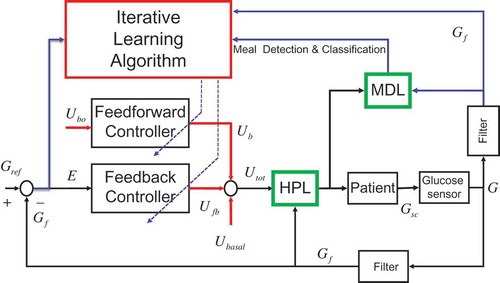
The direct control path features the HDL as an additional module that activates in case a hypoglycemic condition is detected. The HPL block decides whether to interrupt the insulin injection or to limit its rate to the basal value U_basal.

The MDL block monitors the insulin and BG signals with the purpose of detecting the occurrence of possible meals. The MDL output information is used by the outer loop (the ILC module) to coordinate the control and learning actions. The proposed learning scheme can be classified as a mixed direct-indirect approach. The direct part manages the adaptation of the parameters characterizing the feedforward bolus profile U_b whereas the indirect part manages the adaptation of the gains of the feedback controller K_p.

Design Specifications

The objective of the control is to keep the intraday BG concentration within a desired range in presence of uncertainty. In Wang, Dassau, and Doyle (2010) hyperglycemia was defined as a BG concentration greater than 180 mg/dL and significant hypoglycemia was defined as a BG concentration of 60 mg/dL; a BG concentration in the range between 60 and 180 and mg/dL was considered as the safe range for the control of T1DM. The same range was also assumed in the present study to assess the closed-loop control performance. In this study, it was assumed that the patient takes a defined number of meals a day; specifically, we considered three meals: breakfast, lunch, and dinner at nominal times [8, 13, 20] = [t₁, t₂, t₃]; these times define implicitly the meal intervals: [8–13, 13–20, 20–8] = [ΔT₁, ΔT₂, ΔT₃].

The Control Algorithm

This section describes the operations of the blocks in Figure 1. To simplify the explanation, assume for the moment that the meals times [t₁, t₂, t₃] were known. The data acquired during a generic meal interval ΔT_i (i = 1,2,3) are used to drive the learning process for the parameters of the feedback and feedforward controllers that will be applied in the same ΔT_i interval the next day. The proposed scheme allows independently adapting for the parameters of the controllers in the three intervals of the day, which allows, in turn, taking into account possible physiological variation in the meal-glucose-insulin response in the different meal intervals.

During an interval ΔT_i, the administered insulin consists of three contributions: a basal (), a feedforward (), and a feedback () component:

(2)

The quantities in Equation (2) represent insulin administration rates and are expressed in insulin units/hour (U/h); the integer k indicates the day index (repetition cycle index) and t (0 < t < 24) indicates continuous intraday time.

The Basal Contribution

The contribution is a constant basal infusion rate that is designed to keep the fasting BG concentration of the T1DM patient at a nominal fasting steady-state value.

The Feedforward Contribution

The feedforward contribution is a bolus of insulin that is administrated at mealtime t_i whose infusion duration is fixed at Δτ_bi (10 min in this study). The bolus infusion rate is computed according to the formula:

(3)

where the are fixed baseline doses that may take into account therapeutic indications when available. The increments are iteratively adjusted following the learning procedure described in the next sections. In practice, as will be explained shortly, the bolus is activated as soon as the occurrence of a meal is detected at time by the MDL block.

The Feedback Contribution

Because the feedback control contribution is based on the noisy measurement of the glucose sc signal, it was necessary to filter the sensor noise in the before employing the signal in the feedback control law (Saracino, Facchinetti, and Corbelli 2010). A first-order unit gain low-pass filter was used:

(4)

where is the filtered sc glucose signal and t_f is the filter time constant that was fixed at 10 min in this study. Define now the (filtered) sc blood tracking error as: where is the desired reference for the signal (110 mg/dl in this study). The proposed feedback insulin infusion rate is computed with the following derivative law:

(5)

where is the time derivative of the filtered error signal that was computed using the incremental ratio of . The gains in Equation (5) are constrained to be negative so that the insulin administration is active ( is positive) in the time intervals when , namely, when the is increasing. Note that is allowed to be negative but not smaller than the basal infusion rate . The initial value, at day k = 1, for the feedback gains are set to .

The choice of the pure derivative control law in Equation (5) instead of a typical PID control law was based on the considerations made, for example, in Carmen et al. (2005) and in Lam et al. (2002) where, in similar applications, a PD control with heavy emphasis on the derivative term was proposed so that the derivative action dominates the control input during the rise and fall of the BG. The motivation of this approach is that, whereas a proportional controller infuses significant insulin quantities only for high BG levels, heavy derivative control predicts the approach of a high BG level from the steep gradient and infuses insulin preventively, thus enabling a faster response to the increasing BG.

Hypoglycemia Prevention Logic

It is a well-known fact that hypoglycemia is very dangerous for a T1DM patient, especially if it persists for long periods. In order to limit the occurrence of hypoglycemia, a specific HPL was designed. In T1DM, hypoglycemia typically occurs in case an excessive amount of insulin is injected compared to the ingested quantity of CHO. The HPL stops the insulin injection if it detects the approach of a hypoglycemic condition. The HPL block is governed by a rule-based inference engine that decides whether to inhibit the insulin infusion. The HPL is governed by the following two laws:

• Rationale for Law-1: If is decreasing and its value is below a safety threshold (80 mg/dL), then the overall administration is stopped. This action clearly limits the administration of insulin in case the patient is reaching hypoglycemia. The following law is applied

  (6)

• Rationale for Law-2: The overall administration is stopped in case is below 60 mg/dL also in the case is increasing. The following law is applied

  (7)

Meal Detection Logic

In this study, it was assumed that meal announcement information (times t_1,t_2,t₃) are not requested; this implies that the meals’ occurrences have to be estimated, online, from the available signals.

Because the occurrence of a meal typically causes an increase of the BG concentration, the slope of the (filtered) time derivative was, here, employed as the basic signal for meal detection. A well-known problem associated with the employment of the filtered derivative of the sc signal for meal detection originates from the significant noise superimposed to the sc measurement. To limit the occurrence of false meal detections, we propose, here, a nonlinear filtering of the signal that de-emphasizes the amplitude of this signal in the periods that are distant from the nominal mealtimes t_i, while it keeps the signal unchanged around the nominal mealtimes. This filtering strategy produces a robustified signal that is maximally sensitive to the glucose increase in the time intervals when the meal occurrence is likely. To implement this mechanism, the following robustified signal is defined

(8)

where is a sensitivity function that weights the “probability” of a meal occurrence along the 24 hours. In this study, was defined as a combination of bell-shaped functions centered around the nominal mealtimes:

(9)

where is the saturation of the function x(t) at amplitude M. It is immediate to verify that , where the parameter α represents the minimal allowed sensitivity in the 24 hours and σ_i defines the width of the sensitivity period around the nominal ith mealtime. Figure 2 shows the function employed in the simulative section of this article.

FIGURE 2 Sensitivity function p(t,k) for [t₁,t₂,t₃] = [8,13,20], α = 0.4 and σ_i = 0.707h.

The detection of a meal is based on the following binary signal, which is derived from the robustified sc filtered BG:

(10)

where threshold_G is a user-defined value that is tuned such that, in the case that exceeds this threshold, this means that a meal has reasonably occurred or it is still occurring. According to this logic, a meal event occurs in correspondence to the rising edges of the signal. The estimated mealtimes are thus defined as

(11)

The next step, following the detection of a generic meal event at t = t_meal, is the assignment of the meal to one of the three possible classes: breakfast, lunch, or dinner. The class assignment, here, was based on a temporal distance criteria: following a detection, the temporal distances d_i from the nominal mealtimes () are computed, then, t_meal is assigned to the meal leading to the smallest d_i (i = 1: “Breakfast”; i = 2: “Lunch”; i = 3: “Dinner”). The output of the MDL block is, thus, a three-valued logic signal () that triggers the beginning of a specific meal interval that lasts until the detection of the next meal event.

The detected mealtimes are used, in practice, for the online computation of Equations (1–7) in place of the nominal values . This scheme, although simple, proved to be very effective and robust in simulation. Other interesting meal detection strategies were proposed also in Lee et al. (2009) and in Wang, Dassau, and Doyle (2010).

Note 1:

Considering the minimal meal sensitivity coefficient α in the sensitivity function (9), its value should be selected carefully because a very small α can make the system insensitive to overtime meals; therefore, a compromise value should be selected to ensure a reduced number of false alarms while maintaining a sufficient meal sensitivity. In practice, in the experiments we experienced that it is not critical to define an effective compromise sensitive function (see Figure 3).

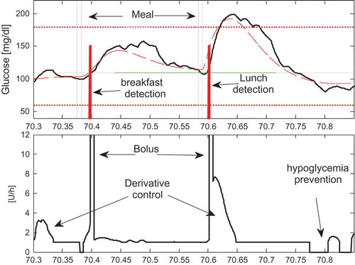
FIGURE 3 (a) The evolution of the BG signal (dotted line), of the s.c measured signal (solid line), the meal “disturbances” and the meal detection signal for Scenario S1 during day 70. (b) The evolution of the overall control signal .

Iterative Learning of the Controller Parameters

In this study, the so-called P-type learning approach (Chien and Liu 1996; Saab 2004) was applied for updating of the controller’s parameters that are the feedforward insulin boluses and the feedback controller gains .

The learning strategy works as follows. Considering a generic day k and a generic detected meal period , the controllers are updated at the end of so that the parametric values that will be used the next day (k+1), in the same time interval ΔT_i,, are those applied in the current day (k) plus a contribution depending on a performance measure that qualifies the system response in the period at day k. The resulting incremental learning rules for the tuning parameters are

(12)

where the gains η_βi and η_ki represent are learning rates; the larger these gains are, the more significant is the effect of the current performance on the learning process. The performance function in is measured as a function of the response of the and of the signals in that period. In detail, the following quantities are used to measure the performance: maximum glucose , minimum glucose , maximum error , minimum error and terminal error at end of the period .

In this study it was assumed, only for the purpose of controller’s tuning, that the target interval for the filtered sc glucose is mg/dL (note that this interval is tighter than the range previously selected for performance evaluation, which is mg/dL). The following strategy defines the performance function .

• In case, during , the control keeps the glucose within the desired range , then the objective of the learning is focused on reducing the terminal value of the tracking error . In this case, the performance function is defined as: .

• In case the control, in some subintervals of , is not able to keep the glucose in the range , then the tuning is focused on the recovery of the safety range for rather than minimizing . In this case, is computed as a combination of the maximum and minimum error according the following rules.

  (13)

Note that in Equation (13), a larger gain is assigned to the violation of the hypoglycemia threshold compared to the gain associated with the violation of the hyperglycemia threshold, because the correction of hypoglycemia is considered a priority over hyperglycemia.

RESULTS

A set of virtual patients and the ILC scheme were implemented in the MATLAB/Simulink environment (Mathworks 2009); a software interface was also developed to set up the parameters that characterize the virtual patients and the controllers.

Virtual Patient Modeling and Control Setup

The proposed ILC was first applied to a prototype T1DM patient that was simulated using the model and the parametric settings given in Dalla Man, Rizza, and Corbelli (2007) and in Magni et al. (2007); in particular, it was considered that an adult of 50 years, 1.75 m in height, weighting 80 Kg, whose glucose-to-insulin sensitivity is 10.8 mg/dL/U (the glucose-to-insulin sensitivity is the maximum glucose drop due to 1 U of insulin). For this patient, the daily Basal Metabolic Rate was computed according the Mifflin rule (Mifflin et al. 1990); and a diet with a 50% content of carbohydrates (resulting in 182 grams/day) was assumed and 4 Kcal for a gram of CHO was considered. The nominal times for the three meals were fixed at [8, 13, 20] = [t₁,t₂,t₃]. The daily CHO amount was partitioned for the three meals according to the percentage: [25%, 37.5%, 37.5%]. The nominal need of daily units of insulin (40 U) was set assuming a need of 0.5 U/Kg (Doran et al. 2005). The 50% of this daily insulin was continuously administrated through the basal contribution and the remaining 50% was divided in 3 fixed bolus contributions according to the percentage [25%, 37.5%, 37.5%].

ILC Setup

The learning algorithm, the HPL, and the MDL blocks were set up as described in the previous sections. As for the learning process, it was assumed that no prior information on the patient is available, therefore, in Equation (12) at day k = 1, it was set at and for i = 1,2,3. The glucose reference was set at 110 mg/dL.

The learning rates in Equation (13) were chosen so that the tuning parameters reach almost stationary values in about a week. Following this guideline, the values were fixed at and based on simulations. Note that is negative since a positive should produce a negative increment of the Kp_i gain. Higher values for the learning rates are not recommended because, in that case, the ILC tends to track the daily fluctuations in the CHO quantities producing overcorrection and/or undercorrection in the administrated insulin. As for the meal detection threshold in Equation (10), this was fixed at 0.4 based on simulative analysis and the parameters defining the sensitivity function in Equation (9) were fixed at σ_i = 0.707 and α = 0.4. These settings were chosen as a compromise solution between a good meal sensitivity and a low level of false alarms (see Note 1).

Control Scenarios

To evaluate and compare the efficacy of the three control contributions in Equation (1), the following control scenarios were analyzed:

• S1: Feedback + Feedforward + HPL+MDL.

• S2: Feedback control only + HPL+MDL.

• S3: Feedforward control only + HPL+MDL.

Scenario S1, which exploits all three contributions, is considered as the reference baseline scenario.

Ideal Conditions

In the first set of experiments, ideal conditions were assumed; in other words, the mealtimes and the CHO amounts for the three meals were assumed constant over time. Quantitative results obtained for the three scenarios derived from long-run simulations of 100 days are reported in Table 1. To avoid the effects of the transients, which typically dominate the first days, the quantitative analysis was restricted to the data collected from the 10th to the 100th day. For each scenario, the percentage of time the patient is in hypoglycemia (%-hypo) and in hyperglycemia (%-hyper) was computed, and the corresponding mean durations of the hypoglycemia and hyperglycemia events. The mean value of the daily BG and of the overall units of administrated insulin is also reported.

TABLE 1 Results in the ideal case for the Scenarios S1, S2, and S3. The analysis considers data starting from the tenth day

	Hypoglycemia		Hyperglycemia		Means		Control Performance (CVGA)					Meal Detection
Scenario	% Hypo	Mean Durat. (min)	% Hyper	Mean Durat. (min)	G (mg/dL)	Insulin (U)	A %	B%	C%	D%	E%	N° false	N° miss	N°corr	Det. Delay (min)
S1 (Proposed)	0	0	0.3	17.4	116.1	47.9	33.5	58.4	0	8.1	0	0	0	270	25.4
S2 (FB. only)	0	0	3.8	54.9	118.0	52.4	33.5	57.3	0	9.2	0	0	0	270	24.9
S3 (FF. only)	0	0	0.7	35.5	118.2	52.7	30.6	58.2	1.3	9.9	0	0	0	270	25,3

To assess the control performance of the scheme the so-called control variable grid approach (CVGA) with the grid partition proposed by Magni et al. (2009) was adopted, where regions A and B means good BG control, regions C and D means over corrections of hypoglycemia/hyperglycemia, and region E means erroneous control (Zarkogiovanni et al. 2011). The CVGA section of Table 1 reports the days, expressed in percentages; the control performance belongs to one of the five regions.

The efficacy of the MDL was measured computing the number of missed meal detections (N°-miss), the number of false meal detections (N°-false) and the number of correct meal detections (N°-corr). Finally, the mean meal detection delay was also computed, which is the mean time between the beginning of a meal and its detection.

Uncertainty on the CHO Quantities

To evaluate the robustness of the control scheme in compensating for uncertainties, a study was carried out that considered increasing levels of uncertainty on the meals times and CHO amounts. In this study, we considered uncertainty as having amplitudes comparable with those considered in Wang, Dassau, and Doyle (2010). In a first study the mealtimes were assumed fixed to the nominal values t_i and uncertainties ranging from ±10% to ±60% of the nominal CHO amounts for the three meals were considered. These uncertainties were induced by adding, to the nominal CHO, uniformly distributed random variables in the interval [±10%, ±60%]. Results achieved for the baseline control scenario S1 are reported in Table 2 (upper).

TABLE 2 (upper) Results in case of uncertainty on the CHO amounts for control scenario S1. (lower) Results in the case of uncertainty on the mealtimes for scenario S1. The analysis considers data starting from the tenth day

		Hypoglycemia		Hyperglycemia		Means		Control Performance (CVGA)					Meal Detection
Meal Time Uncert	CHO Uncert	% Hypo	Mean Durat. (min)	% Hyper	Mean Durat. (min)	G (mg /dL)	Insulin (U)	A %	B%	C%	D%	E%	N° false	N° miss	N° corr	Det. Delay (min)
0	± 10%	0	0	4.3	52.4	118.3	52.3	33.5	58.4	0	8.1	0	0	0	270	24.8
0	± 20%	0	0	5.2	54.3	118.8	52.0	33.5	57.3	0	9.2	0	0	0	270	24.3
0	± 30%	0	0	5.9	66.2	118.5	52.0	30.6	58.2	1.3	9.9	0	0	0	270	23.2
0	± 40%	0	0	6.9	77.7	119.0	51.9	23.2	64.9	1.4	10.5	0	0	0	270	23.1
0	± 50%	0	0	7.9	85.6	119.9	51.6	14.4	69.1	2.8	13.7	0	0	0	270	24.9
0	± 60%	0	0	8.9	88.6	120.6	51.5	9.9	69.0	5.6	15.1	0.4	0	0	270	24.4
± 10 m	0	0	0	4.4	72.0	123.3	50.4	33.1	60.9	0	6.0	0	0	0	270	23.3
± 20 m	0	0	0	5.2	80.8	122.1	50.4	30.6	55.6	5.3	8.5	0	3	0	270	23.0
± 30 m	0	0	0	6.1	80.1	121.4	50.0	29.7	52.4	5.7	12.2	0	5	0	270	23.2
± 40 m	0	0.1	66.0	6.8	77.9	121.0	50.2	31.1	42.8	12.0	14.1	0	6	0	270	23.3
± 50 m	0	0.2	63.0	7.4	78.2	121.0	49.1	30.0	43.1	13.0	13.9	0	8	0	270	23.7
± 60 m	0	0.1	57.5	8.4	77.8	120.5	49.5	32.2	39.2	15.1	13.5	0	10	0	270	24.7

Uncertainty on the Mealtimes

In this experiment, the CHO amounts were assumed fixed to the nominal values while uncertainties ranging from ±10 to ±60 min were considered, adding independent uniformly distributed random variables to the nominal t_i. Results for control scenario S1 are reported in Table 2 (lower).

Joint Uncertainty on the Mealtimes and CHO Amounts

In a realistic context, both the mealtimes and CHO amounts can vary independently, therefore, it is of interest to evaluate the performance in presence of joint uncertainties. An analysis was carried out considering maximum uncertainties of 40 min on the nominal mealtimes t_i and maximum uncertainties of 50% on the nominal CHO quantities for the three meals. These ranges are deemed to be adequate to capture realistic uncertainties (Wang, Dassau, and Doyle 2010). This challenging context is particularly suited also for the evaluation of the efficacy of the HPL block; for this reason it was introduced as an additional control scenario in which the HPL is disabled (only for comparison purpose):

• S4: Feedback + Feedforward + MDL, HPL (disabled).

Quantitative results for the scenarios S1, S2, S3, and S4 are summarized in Table 3 (upper).

TABLE 3 Results in the case of joint uncertainty on the mealtimes ( 40 min) and on the CHO amounts ( 50%) for scenarios S1, S2, S3, and S4; in the case of variable profiles for the glucose sensibility (scenarios S5 and S6); in the case of pure PD control (S7) and in case of manual control (S8). The analysis considers data starting from the tenth day

	Hypoglycemia		Hyperglycemia		Means		Control Performance (CVGA)					Meal Detection
Scenario	% Hypo	Mean Durat. (min)	% Hyper	Mean Durat. (min)	G (mg/dL)	Insulin (U)	A %	B %	C %	D %	E %	N° false	N° miss	N° corr	Det. Delay (min)
S1 (proposed)	0.3	72.6	6.3	81.9	120.2	50.5	19.5	53.7	11.1	15.7	0	11	2	268	25.0
S2 (FB. only)	2.0	116.6	8.1	76.8	117.6	47.4	21.2	52.0	0.7	26.1	0	13	3	267	27.8
S3 (FF. only)	1.1	104.4	9.8	100.4	119.5	49.8	13.2	47.9	25.4	13.5	0	15	8	262	29.7
S4 (no HPL)	1.8	116.2	6.9	88.1	119.6	49.6	18.7	51.3	12.3	17.4	0.3	15	4	266	28.5
S5 Linear	0.5	81.0	6.6	88.0	119.1	52.4	22.2	52.3	10.1	14.7	0.7	12	1	269	27.2
S6 Sinusoid	2.6	104.9	9.6	95.1	120.2	54.0	18.0	51.7	12.3	17.7	0.3	14	1	269	26.3
S7 (PD+ FF)	3.6	92.2	10.7	85.8	109.9	55.2	11.3	40.2	41	5.5	2	16	9	261	29.2
S8 (Manual)	0	0	6.0	79.2	117.7	51.5	14.6	75.5	1.7	8.0	0	0	0	300	0

Time-Varying Insulin Sensitivity

Previous studies were carried out assuming a constant glucose-to-insulin sensitivity for the virtual patient. In practice, the insulin sensitivity can vary due to many endogenous and exogenous causes, therefore, it is of interest to evaluate the performance of the learning control scheme assuming time-dependent insulin sensitivity profiles.

Considering the adaptation properties of the ILC scheme, it should be noticed that, because the duration of the repetition cycles is 24 h, the proposed learning scheme is not suitable to compensate for dynamic changes having a shorter period, such as intraday insulin sensitivity variations. This fact can be appreciated when observing that the scheme requires a horizon of some days (repetitions) to reach the almost steady-state values both for the feedforward and for the feedback control gains (see Figure 5). It should be also observed that, due to this limitation, an increase of the adaptation learning rates in Equation (22), in the attempt to track fast dynamics, might be ineffective and even dangerous, causing excessive oscillations in the control signal. For these reasons, the following analysis was carried out considering dynamic changes with a period longer than one day. The effects of a time-varying insulin sensitivity were simulated by varying the parameter expressing the insulin effect on glucose utilization. In the first study, a linear variation of the parameter was introduced along the 100 days starting from –60% and reaching +60% the last day.

FIGURE 4 (a) Evolution of the meal sensitivity function at day 89. (b) Evolution of the signal (dotted line), of (solid line) and of the binary meal detection signal.

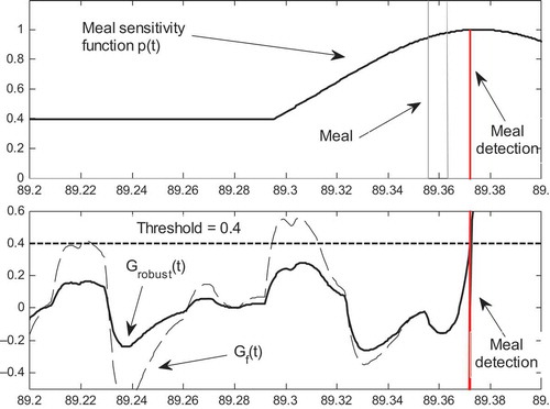
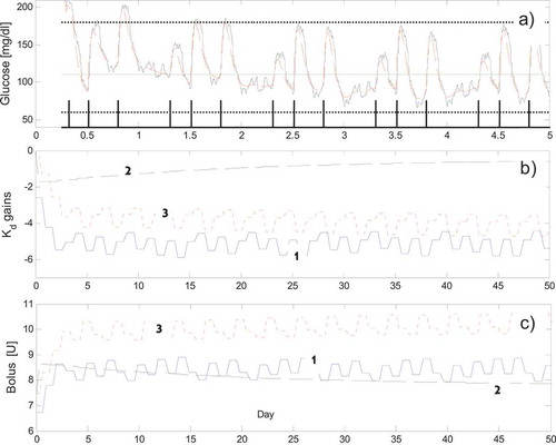
FIGURE 5 (a) The BG response (dotted line) and the measured sc in the first five days (ideal case, S1). The upper horizontal line indicates the 180 mg/dL limit, the lower line indicates the 60 mg/dL; the 110 mg/dL line indicates the reference signal; the binary meal detection signal generated by the MDL block is also shown. (b) The adaptation of the three feedback gains in the first 50 days. (c) The adaptation of the total amount of insulin boluses in the first 50 days (1 = “breakfast,” 2 = “lunch,” 3 = “dinner”).

In a second study, a sinusoidal variation with amplitude 60% of the nominal value and a period of 10 days was superimposed to the nominal value. The two control scenarios are defined as follows:

• S5: (Feedback + Feedforward + HPL+MDL) + Linear variation of the insulin sensitivity from –60% to +60% in 100 days.

• S6: (Feedback + Feedforward + HPL+MDL) + additive sinusoidal variation of the insulin sensitivity with amplitude 60% of the nominal value (period 10 days).

In scenarios S5 and S6, the same joint uncertainties used in S4 were applied for the mealtimes and for the CHO amounts. Table 3 (lower) reports the results for scenarios S5 and S6.

Comparison with a Standard PD Control Strategy

The performance of the ILC controller was also compared to those of a standard fixed gain PD controller assuming that the feedforward pre meal boluses and the basal insulin are fixed to the nominal values while the joint uncertainty for the mealtimes and for the CHO amounts are the same of S4. The implemented PD control law was defined as follows: . Because the system under investigation is strongly nonlinear with an hard constraint on the sign of the control signal, the tuning of the PD controller was performed by trials and error through a simulation study. The starting value for the derivative control gain K_d was fixed at the mean value achieved in scenario S1 while the proportional gain K_p was incrementally decreased starting from zero. The objective of the tuning was to select a PD controller that maintains the glucose concentration in the desired range most of the time avoiding, as much as possible, long periods of hyperglycemia and hypoglycemia. The values selected for the gains were K_p = −0.05 and K_d = −5. The following scenario is defined for the standard PD control:

• S7: PD control: (HPL disabled, bolus adaptation disabled, MDL enabled).

It should be noted that Scenario S7 (still) requires the operation of the MDL block to detect meals and to command the administration of the feedforward insulin bolus. Results for scenario S7 are reported in Table 3 (lower).

Comparison with a Manual Feedback/Feedforward ILC

In the case when one renounces to the autonomy of the ILC scheme, allowing the interaction by the patient to indicate the beginning of the meal intervals, then, the scheme simplifies because the MDL block is no longer necessary with the important advantage that the meal detection delay and false alarms are zeroed. Therefore it is of interest to evaluate the possible performance improvement produced in the case of a “manual” ILC operation comported to the fully autonomous scenario S1. The following “manual” scenario is defined:

• S8: Feedback + Feedforward + HPL (MDL disabled: the beginning of the meals is manually indicated by the patient).

In this scenario the feedforward bolus is injected as soon the patients announces the beginning of the meal; results for scenario S8 are reported in Table 3 (lower).

Interpatient Performance

A final study was performed examining the interpatient performance. For this purpose, a set of additional eight virtual diabetic subjects was implemented with the parametric values in the ranges suggested by Kovatchev et al. (2009). The main features of the nine subjects are reported in Table 4; these represent a significant class of subjects characterized by a large spectrum of the glucose to insulin sensitivity index. The performance achieved in case on joint meal and CHO uncertainty are reported in Table 5.

TABLE 4 The main features for the nine subjects. The glucose-to-insulin sensitivity is defined as maximum glucose drop due to 1 U of insulin

Subject	1	2	3	4	5	6	7	8	9
Glucose to insulin sensitivity (mg/dL/U)	10.8	13.2	8.7	4.5	5.5	3.5	28.9	34.6	23.6
Nominal Daily Insulin (U)	39.8	26.1	59.3	39.8	26.1	59.3	39.8	26.1	59.3
Nominal Daily CHO (g)	181.6	150.8	225.5	181.6	150.8	225.5	181.6	150.8	225.5

TABLE 5 Results in the case of joint uncertainty on the mealtimes ( 40 min) and on the CHO amounts (50 %) for scenario S1 for the nine patients. The analysis considers data starting from the tenth day

	Hypoglycemia		Hyperglycemia		Means		Control Performance (CVGA)					Meal Detection
Patient	% Hypo	Mean Durat. (min)	% Hyper	Mean Durat. (min)	G (mg/dL)	Insulin (U)	A %	B %	C %	D %	E %	N° false	N° miss	N° corr	Det. Delay (min)
P-1 (nominal)	0.3	72.6	6.3	81.9	120.2	50.5	19.5	53.7	11.1	15.7	0	11	2	268	25.0
P-2	0.7	116.1	8.7	91.1	121.1	5027	5.0	56.3	2.8	33.1	2.8	15	3	267	27.1
P-3	0.3	61.1	5.0	73.2	120.7	46.2	3.5	90.8	2.0	3.7	0.0	8	1	269	20.1
P-4	0.9	67.9	9.4	109.1	123.3	78.7	6.0	70.5	0	20.5	2.9	16	3	267	10.4
P-5	2.8	95.8	11.5	113.4	130.7	78.5	5.5	40.8	0	43.2	10.5	18	4	266	12.7
P-6	0.6	80.3	7.5	100.1	120.1	79.9	4.7	82.3	0	13.0	0	11	3	267	10.1
P-7	0.2	59.1	5.5	74.3	124.3	32.6	6.1	70.6	2.6	20.9	0	9	2	268	34.8
P-8	0.4	32.0	6.8	80.1	126.3	30.1	3	53.6	11.9	28.0	3.5	11	2	268	35.1
P-9	0.1	55.1	3.4	55.2	122.1	39.0	5.3	75.2	1.1	18.4	0	6	1	269	32.2

DISCUSSION

Before discussing the results it is useful to analyze the operation of the proposed ILC strategy during normal operation. For this purpose, in Figure 3 it is shown the evolution of the BG signal (dotted line), of the sc-measured signal (solid line), of the administrated insulin and of the meal detection signal during a sample day (day 70) in case of Scenario S1. Specifically in Figure 3, two consecutive meal “disturbances” cause the increase of the BG. The MDL, following a short delay, detects the occurrence of the meals classifying the first as a breakfast and the later as a lunch. Immediately after the detections it is enabled the administration of the breakfast and of the lunch boluses respectively (Figure 3(b)). In these periods also the feedback derivative controllers continuously inject their portion of insulin. Note that at time 70.77 falls below 70 mg/dL and the HPL stops immediately the injection of insulin. It should be also noticed that the oscillations in the administrated feedback insulin arise from the sc sensor noise. This effect could be easily reduced by increasing the filter time constant associated to the filter at the price of causing a delay in the control action that could weaken the typical anticipatory effects of the derivate control strategy. However it should be also observed that, thanks to the natural lowpass filtering property of the insulin-glucose system, the control signal oscillations do not have any practical effect on the actual GB concentration that remains substantially smooth. Therefore the current setting of the filer is deemed adequate for the current application.

As for the MDL operation, Figure 4(a) shows the evolution of the of meal sensitivity signal at day 89. As expected the sensitivity is low (40%) in the time interval that is far from the nominal mealtime, while reaches the 100% around the nominal mealtime. Figure 4(b) shows the evolution of the , of and of the meal detection binary signal. It can be observed that, far from the meal, the signal remains well below the threshold while the signal causes two false meal detections before time 89.30. As the nominal mealtime approaches the signal get closer to and from time 89.35 the two signals are almost undistinguishable. Both signals detect the “true meal” at time 89.375, thus proving the efficacy of the proposed scheme in preventing false alarms without penalizing the meal detection capacity.

Ideal Conditions

Results in Table 1 indicate that control scenarios S1 and S3 are particularly effective in fact no hypoglycemia and moderate hyperglycemia episodes (less than 0.7%) were observed, while, in case of pure feedback control (scenario S2), a significant degradation results in the control of hyperglycemia (%Hyper about 4%). Last consideration revels, implicitly, the importance of the feedforward bolus in decreasing the number of hyperglycemic events even if the bolus is administered following a mean meal detention delay of about 25 min. As for the performance of the MDL block this resulted particularly effective in fact all the 270 meals were correctly detected without false alarms or wrong detections.

In Figure 5(a), it is shown the evolution of the BG and of the measured sc BG signals along with the meal detection binary signal t_meal computed by the MDL for the first 5 days. Note that, following an initial transitory phase, the BG enters and remains within the desired range mg/dl. Figure 5(b) shows the adaptation of the feedback controller’s gains for the three time intervals ΔT₁, ΔT₂ and ΔT₃. It can be observed that the gains stabilize to almost stationary values in about a week; similarly, Figure 5(c) shows the adaptation of the total amount of the feedforward insulin bolus for the three meals. The ripple superimposed to the and signals originates, mainly, from the stochastic sc sensor noise. As for the control performance the CVGA produced results mainly in the A and B regions proving that the control performance can be deemed satisfactory for the three scenarios. In conclusion, for this ideal context, results indicate that control scenario S1 and S3 are the most effective revealing that a bolus based feedforward control might be sufficient to provide a good BG control. This fact is not surprising since the effect of the feedback control is expected to be important mainly in presence of uncertainties.

Uncertainty on the CHO Quantities

Considering the study dealing with the uncertainty in the CHO amounts, data in Table 2 (upper) highlight a remarkable robustness of the scheme in avoiding hypoglycemia in fact no event was reported even for a ± 50% uncertainty. An almost linear worsening effect was instead observed for the hyperglycemia compensation performance; for instance, an uncertainty of ±60% produced a 8.9 %-hyper index. Note that the daily mean BG and the mean meal detection delay do not increase with the amplitude of the meal uncertainty. The scheme shows also a remarkable robustness in terms of meal detection ability and avoidance of false alarms; conversely there is an increase of the mean duration of the hyperglycemia events with the increase of the uncertainty.

Uncertainty on the Mealtimes

As for the study dealing with the uncertainty in the mealtimes, data in Table 2 (lower) confirm the efficacy in avoiding hypoglycemia for uncertainties smaller or equal to ±30 min, while modest hypoglycemia events appear only with uncertainties larger than ±40 min. The good performance in terms of hypoglycemia prevention has an impact on the capacity of compensating for hyperglycemia that indeed produced a %-hyper time indexes ranging from 4.4% to 8.4%. This fact can be rationally explained noting that in Equation (13) it was intentionally decided to assign a higher penalty to the violations of the hypoglycemia threshold compared to the penalty assigned to hyperglycemia violation. The logical effect is that the learning algorithm “favors” hyperglycemia events in order to prevent, as much as possible, hypoglycemia. A more balanced performance could be achieved by decreasing the hypoglycemia penalty at the cost of increasing the occurrence of hyperglycemia. Because of the uncertainty in the mealtimes, it is also observed that the scheme is no longer able to avoid false meal detections whose number, indeed, increases with increasing uncertainties; conversely, the scheme is still able to detect correctly all the meals.

Joint Uncertainty on the Mealtimes and CHO Amounts

Considering the case of joint uncertainty on the mealtimes and on the CHO quantities (Table 3, upper), the best performances were achieved in the control scenario S1. In more detail, S1 is better than S2 in the hypoglycemia management, in fact, S1 produced a remarkable 0.3%-hypo time index whereas S2 and S3 produced a much higher value of 2.0% and 1.1%, respectively. For S2 and S3, the extension of the mean time duration of the hypo events is also noticed. The evolution of the BG in scenario S1 is shown in Figure 6(a).

FIGURE 6 (a) The BG response in the first 30 days for the Scenario S1. (b) Scenario S5. (c) Scenario S6.

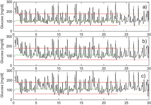
The comparative analysis of the results reveals that, in contrast to the ideal case (Table 1), the performances of scenario S1 are definitely better than those of control scenarios S2 and S3. This fact is important because it proves the superior performance of the proposed mixed feedback/feedforward strategy in compensating for realistic mixed uncertainties compared to a pure feedback or to a pure feedforward control scheme.

Considering scenario S4, the disabling of the HPL block causes the %-hypo time index to increase from 0.3 to 1.8, while the %-hyper index remains substantially unchanged. This fact highlights the efficacy of the HPL block in decreasing the hypoglycemia events without increasing, significantly, the occurrence of hyperglycemia.

As for the performance of the MDL, a satisfactory robustness of the meal detection algorithm is still observed in terms of the high number of correct meal detections, the small number of missed meals, and the limited number of false meal detections; a small increase in the mean meal detection delay compared to the ideal case is also noticed.

In conclusion, considering the significant magnitude of the joint uncertainties and the fact that the control performance falls mainly in the A, B, and C regions, the robustness of the control scenario S1 can be considered acceptable and comparable with the results reported for example in Wang, Dassau, and Doyle (2010).

Note 2:

A deep analysis of the operation in scenario S1 reveals that one possible cause of the hyperglycemia originates from the false meal detections that enable, incorrectly, the administration of unnecessary boluses of insulin. However, it should be also observed that, in the event the HPL block detects the approach of hypoglycemia, the administration of insulin is immediately stopped. Therefore, the HPL block also provides a natural and effective remedy to counteract the effect of the false alarms that unavoidably can occur in a completely autonomous conduction.

Note 3:

As a general observation, considering the performance of the ILC scheme in the first days (see Figure 5), the initial transitory is strongly influenced by the conservative assumption that no prior information on the patient response is available; that is, at day k =1, it was assumed that and . In practice, it can be reasonable to assume that the initial values for these parameters can be scheduled as a function of the patient glucose-to-insulin sensitivity. In this case, it is expected that there is a significant speedup in the stabilization of the BG and of the adaptive parameters of the controllers since the first day.

Time-Varying Insulin Sensitivity

Good results were also achieved in the case of time-varying insulin effect on glucose utilization for scenario S5 (linear) whose BG response is shown in Figure 6(b). In fact, it can be observed that the responses in Figure 6(a) (with constant insulin sensitivity) and in Figure 6(b) are comparable, proving the excellent capacity of the ILC scheme in compensating for a linear time-varying glucose sensitivity. A performance reduction is instead observed in scenario S6 shown in Figure 6(c), where it can be noticed that the control is not fully able to compensate for the effect of the sinusoidal time-varying glucose sensitivity that is confirmed by the increase of the %-hypo index in Table 3. Overall, the above results highlight the capacity of the ILC scheme in compensating for time-varying glucose sensitivity, but only in the case of slow time-varying effects.

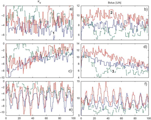
Figure 7 shows the adaptation, during the 100 days, of the feedback gains and of the total feedforward insulin boluses for scenarios S1, S5, and S6, respectively, in the case of joint uncertainties. Note that because the significant uncertainties and because of the sc glucose sensor noise, the adaptive parameters do not reach almost-stationary steady values as in the ideal case. In particular, in the case of scenarios S5 and S6, a linear and sinusoidal trend is perceived during the 100 days, testifying to the correct activity of the learning scheme in compensating for linear and sinusoidal time-varying glucose sensitivities.

FIGURE 7 (a–b) The adaptation of the three feedback gains and of the total amount of insulin boluses during the 100 days for Scenario S1 in the first 50 days. (1 = “breakfast,” 2 = “lunch,” 3 = “dinner”). (c–d) Scenario S5: linear glucose sensitivity variation. (e–f) Scenario S6: sinusoidal glucose sensitivity variation.

Comparison with a Standard PD Control Strategy

Considering scenario S7, the PD control scheme + FF boluses produced a significant degradation of performance not only in terms of the %-hyper and %-hypo time indexes but also in terms of the increase of the mean duration of the hyper and hypo events. This fact clearly reflects the difficulty of a single fixed gain PD controller in compensating satisfactorily both hyperglycemia and hypoglycemia in the presence of significant nonlinearities and uncertainties.

Comparison with a Manual Feedback/Feedforward ILC

Considering the manual scenario S8, it can be observed that the %-hyper index remains essentially equivalent to the fully autonomous scenario S1, highlighting the important fact that the meal detection delay, which is unavoidable in the autonomous control scenario S1, does not cause a significant performance decrease in terms of the hyperglycemia avoidance capabilities compared to the operation with manual meal announcement. However, it is remarked that, under manual conduction (S8), it is possible to avoid, completely, the occurrence of hypoglycemia. The mechanism that induces hypoglycemia under autonomous conductions and the role of the HPL in preventing hypoglycemia has been described in Note 2.

Interpatient Performance

Analyzing the results of the proposed ILC applied to the population of nine diabetic patients, Table 5 indicates that, despite the significant joint uncertainties, the ILC scheme is still effective in the control of hypoglycemia because the %-hypo index is less than 1% for most patients. The most problematic patients are those having the lower insulin-to-glucose sensitivity (subjects 4, 5, and 6) that produced a %-hyper index in the range 5%–12%. Analyzing the CVGA performance, it can be noticed that some patients have a control performance in the E region (“erroneous control”) with a percentage larger than 5%; for these patients it can be deduced that the ILC scheme might not be robust enough to counteract very large joint uncertainties. However, considering the significant magnitude of the considered uncertainties, the overall interpatient performance for the noncritical patients can be considered acceptable and comparable with the results reported, for example, in Wang, Dassau, and Doyle (2010).

CONCLUSIONS

The application of a novel Iterative Learning Scheme relying on a mixed feedback and feedforward control strategy was proposed to control the blood glucose in Type 1 diabetes. Through a simulation study, it was shown that the scheme is able to learn, day by day, the insulin-glucose response of a T1DM patient and it is also able to detect and classify the occurrence of a meal. As a consequence, in some days, the scheme is able to control the subcutaneous insulin administration keeping the BG in the safety range. The most relevant feature of the learning scheme is its high level of autonomy; in fact, it does not require any mathematical model of the patient for controller design and tuning purposes and does not require any a priori meal announcement information, nor the estimation of ingested carbohydrates or the computation of the insulin premeal boluses. Long-term simulation studies showed that the proposed ILC scheme provides satisfactory performance even in the presence of significant joint uncertainties on the mealtimes and on the amount of ingested CHO. A comparative analysis proved that the proposed ILC scheme provides better performances than simpler ILC solutions based on pure feedback or on pure feedforward control strategies; in addition, the scheme performs significantly better than a standard PD control scheme, especially in the management of hypoglycemia and in the reduction of the number of hyperglycemia and hypoglycemia events. The learning scheme has also shown a remarkable capacity to counteract a slowly time-varying insulin effect on glucose utilization.

Intersubjects variability, in particular the patient glucose-to-insulin sensitivity, plays a relevant role on the control performance, in particular, simulation studies revealed that subjects having a glucose-to-insulin sensitivity less that 5.5 (mg/dl/U) are the most problematic to control; similarly, for low-weight subjects, the control can induce overcorrection of the BG concentration. For the nominal subjects and for noncritical patients, the control performance of the ILC scheme are deemed appropriate also in the case of significant joint time/CHO uncertainties.

REFERENCES

- Abu-Rmileh, A., and W. Garcia-Gabin. 2010. Feedforward-feedback multiple predictive controllers for glucose regulation in type 1 diabetes. Computer Methods and Programs in Biomedicine 99(1):113–123.
- Alpaydin, E. 2004. Introduction to machine learning. Cambridge, MA, USA: The MIT Press.
- Bequette, B. W. 2005. A critical assessment of algorithms and challenges in the development of a closed-loop artificial pancreas. Diabetes Technology & Therapeutics 7(1):28–47.
- Bondia, J., E. Dassau, H. Zisser, R. Calm, J. Vehí, L. Jovanovič, and F. J. Doyle. 2009. Coordinated basal–bolus infusion for tighter postprandial glucose control in insulin pump therapy. Journal of Diabetes Science and Technology 3(1):89–97.
- Boyne, M., D. Silver, J. Kaplan, and C. Saudek. 2003. Timing of changes in interstitial and venous blood glucose measured with a continuous subcutaneous glucose sensor. Diabetes 52:2790–2794.
- Breton, M., and B. P. Kovatchev. 2008. Analysis modeling and simulation of the accuracy of continuous glucose sensors. Journal of Diabetes Science and Technology 2(5):853–862.
- Carmen, V., C. V. Doran, J. G. Chase, G. M. Shaw, K. T. Moorhead, and N. H. Hudson. 2005. Derivative weighted active insulin control algorithms and intensive care unit trials. Control Engineering Practice 13:1129–1137.
- Chien, C. J., and J. S. Liu. 1996. A P-type iterative learning controller for robust output tracking of nonlinear time-varying systems. International Journal of Control 64(2):319–334.
- Clemens, A.H., P. H. Chang, and R.W. Myers. 1997. The development of Biostator. A glucose controlled insulin infusion system (GCIIS). Hormone and Metabolic Research 7:23–33.
- Cobelli, C., C. Dalla Man, G. Sparacino, L. Magni, G. De Nicolao, and B. P. Kovatchev. 2009. Diabetes: models. Signals and control. IEEE in Reviews Biomedical Engineering 2(1):54–96.
- Cominos, P. 2002. PID controllers: Recent tuning methods and design to specification. IEE Proceedings— Control Theory and Applications 149(1):46–53.
- Dalla Man, C., D. M. Raimondo, R. A. Rizza, and C. Cobelli. 2007. GIM Simulation software of meal glucose-insulin model. Journal of Diabetes Science and Technology 1(3):323–330.
- Dalla Man, C., M. Camilleri, and C. Cobelli. 2006. A system model of oral glucose absorption: Validation on gold standard data. IEEE Transactions in Biomedical Engineering 53(12):2472–2478.
- Dalla Man, C., R. A. Rizza, and C. Cobelli. 2007. Meal simulation model of the glucose-insulin system. IEEE Transactions in Biomedical Engineering 54(10):1740–1749.
- Doran, C. V., J. G. Chase, G. M. Shaw, K. T. Moorhead, and N. H. Hudson. 2005. Derivative weighted active insulin control algorithms and intensive care unit trials. Control Engineering Practice 13(9):1129–1137.
- Dua, P., F. J. Doyle, and E. N. Pistikopoulos. 2009. Multi-objective blood glucose control for type 1 diabetes. Medical & Biological Engineering & Computing 47(3):343–352.
- Elleri, D., D. B. Dunger, and R. Hovorka. 2011. Closed-loop insulin delivery for treatment of type 1 diabetes. BMC Medicine 9:120.
- Fravolini, M. L., and P. Fabietti. 2013. An iterative learning strategy for the auto-tuning of the feedforward and feedback controller in type-1 diabetes. Computer Methods in Biomechanics and Biomedical Engineering, (in press). Available at http://dx.doi.org/10.1080/10255842.2012.753064
- Good, R., J. Hahn, T. Edison, and S. J. Qin. 2002. Drug dosage adjustment via run-to-run control. In Proceedings of the American Control Conference 4044–4049. IEEE.
- Klonoff, D. C. 2005. Continuous glucose monitoring: Roadmap for 21st century diabetes therapy. Diabetes Care 28(5):1231–1239.
- Kovatchev, B. P., M. Breton, C. Dalla Man, and C. Cobelli. 2009. In silico preclinical trials: A proof of concept in closed-loop control of type 1 diabetes. Journal of Diabetes Science and Technology 3(1):44–55.
- Kulcu E., J.A. Tamada,G. Reach,R.O. Pott, M.J. Lesho. 2003. Physiological differences between interstitial glucose and blood glucose measured in human patients. Diabetes Care 26:2405–2409.
- Lam, Z. H., K. S. Hwang, J. Y. Lee, J. G. Chase, and G. C. Wake. 2002. Active insulin infusion using optimal and derivative–weighted control. Medical Engineering & Physics 24(10):663–672.
- Leal, Y., W. Garcia-Gabin, J. Bondia, E. Esteve, W. Ricart, J. M. Fernández-Real, and J. Vehí. 2010. Real-time glucose estimation algorithm for continuous glucose monitoring using autoregressive models. Journal of Diabetes Science and Technology 4(2):391–403.
- Lee, H., B. A. Buckingham, D. M. Wilson, and B. W. Bequette. 2009. Closed-loop artificial pancreas using model predictive control and a sliding meal size estimator. Journal of Diabetes Science and Technology 3(5):1082–1090.
- Magni, L., D. M. Raimondo, C. Dalla Man, G. De Nicolao, B. Kovatchev, and C. Cobelli. 2007. Model predictive control of type 1 diabetes: An in silico trial. Journal of Diabetes Science and Technology 1(6):804–812.
- Magni, L., D. M. Raimondo, C. Dalla Man, G. Nicolao, B. Kovatchev, and B. C. Cobelli. 2009. Model predictive control of glucose concentration in type I diabetic patients: An in silico trial. Biomedical Signal Processing and Control 4(4):338–346.
- Marchetti, G., M. Barolo, L. Jovanovic, H. Zisser, and D. E. Seborg. 2008. An improved PID switching control strategy for type 1 diabetes. IEEE Transactions in Biomedical Engineering 55(3):857–865.
- Mifflin, D. M., S. T. Jeor, L. A. Hill, B. J. Scott, S. A. Daugherty, and Y. O. Koh. 1990. A new predictive equation for resting energy expenditure in healthy individuals. American Journal of Clinical Nutrition 51(2):241–247.
- Palerm, C. C., H. Zisser, L. Jovanovic, and F. J. Doyle. A run-to-run control strategy to adjust basal insulin infusion rates in type 1 diabetes. 2008. Journal of Process Control 18(3–4):258–265.
- Rossetti, P., J. Bondia, J. Vehí, and C. G. Fanelli. 2010. Estimating plasma glucose from interstitial glucose: the issue of calibration algorithms in commercial continuous glucose monitoring devices. Sensors 10(12):10936–10952.
- Saab, S. S. 2004. On the P-type learning control. IEEE Transactions on Automatic Control 39(11):2298–2302.
- Saracino, G., A. Facchinetti, and C. Corbelli. 2010. Continuous glucose monitoring sensors: On-line signal processing issues. Sensors 10: 6751–6772.
- Schubert, W., P. Baurschmidt, J. Nagel, R. Thull, and M. Schaldach. 1980. An implantable artificial pancreas, Medical & Biological Engineering & Computing 18(4): 527–537.
- Steil, G. M., K. Rebrin, C. Darwin, F. Hariri, and M. F. Saad. 2006. Feasibility of automating insulin delivery for the treatment of type 1diabetes. Diabetes 55(12):3344–3350.
- The MathWorks Inc. 2009. Robust Control Toolbox Users’s Guide. Available at http://www.mathworks.com/access/helpdesk/help/toolbox/
- Wang, Y., E. Dassau, and F. J. Doyle. 2010. Closed-loop control of artificial pancreatic b-cell in type 1 diabetes mellitus using model predictive iterative learning control. IEEE Transactions on Biomedical Engineering 57(2):211–219.
- Wang, Y., E. Dassau, H. Zisser, L. Jovanovič, and J. F. Doyle. 2010. Automatic bolus and adaptive basal algorithm for the artificial pancreatic β-cell. Diabetes Technology and Therapeutics 12(11): 879–887.
- Wang, Y., F. Gao, and F. J. Doyle. 2009. Survey on iterative learning control, repetitive control and run-to-run control. Journal of Process Control 19(10):1589–1600.
- Wang, Y., H. Zisser, E. Dassau, L. Jovanovič, and F. J. Doyle. 2010. Model predictive control with learning-type reference: Application in artificial pancreatic β-cell. American Institute of Chemical Engineers Journal 56(6):1510–1518.
- Weinzimer, S. A., G. M. Steil, K. L. Swan, J. Dziura, N. Kurtz, and W. V. Tamborlane. 2008. Fully automated closed-loop insulin delivery versus semiautomated hybrid control in pediatric patients with type 1diabetes using an artificial pancreas. Diabetes Care 31(5):934–940.
- Wild, S., G. Roglic, A. Green, R. Sicree, and H. King. 2004. Global prevalence of diabetes estimates for the year 2000 and projections for 2030. Diabetes Care 27(5):1047–1053.
- Xu, J. X., and D. Huang. 2007. Optimal tuning of PID parameters using iterative learning approach. In Proc. IEEE 22 International Symposium on Intelligent Control, 226–231. IEEE.
- Youssef, J. E, J. Castle, and W. K. Ward. 2009. A review of closed-loop algorithms for glycemic control in the treatment of type 1 diabetes. Algorithms 2(1):518–532.
- Zarkogianni, K., A. Vazaiou, S. G. Mougiakakou, A. Prountzou, and K. S. Nikita. 2011. An insulin infusion advisory system based on auto-tuning nonlinear model predictive control. IEEE Transactions on Biomedical Engineering 58(9):2467–2477.